




Abstract
This study shows that residual variation can cause problems related to scaling in exponential random graph models (ERGM). Residual variation is likely to exist when there are unmeasured variables in a model—even those uncorrelated with other predictors—or when the logistic form of the model is inappropriate. As a consequence, coefficients cannot be interpreted as effect sizes or compared between models and homophily coefficients, as well as other interaction coefficients, cannot be interpreted as substantive effects in most ERGM applications. We conduct a series of simulations considering the substantive impact of these issues, revealing that realistic levels of residual variation can have large consequences for ERGM inference. A flexible methodological framework is introduced to overcome these problems. Formal tests of mediation and moderation are also proposed. These methods are applied to revisit the relationship between selective mixing and triadic closure in a large AddHealth school friendship network. Extensions to other classes of statistical work models are discussed.
Over the past decade, social scientists have increasingly looked to statistical network methods to address important substantive questions. These methods improve upon classical approaches of statistical inference for network data by relaxing independence assumptions and providing a means to formally represent interdependent social phenomena. Among the models available, exponential random graph models (ERGM) have established themselves as an especially popular tool for this type of inference given their flexibility and ability to represent nodal, dyadic, and network covariates. Indeed, the diffusion of ERGM across the social, political, behavioral, and health sciences has led to an explosion of research examining the generative properties of social networks (Adams and Schaefer 2016; Cranmer et al. 2017; Kreager et al. 2017; Lewis 2013; Papachristos, Hureau, and Braga 2013; Young 2011).
However, there is a problem in ERGM applications that has gone largely unnoticed: ERGM coefficients are confounded with residual variation–unexplained variation in tie probabilities—that rescales model coefficients. This has several important consequences. First, coefficients and exponentiated coefficients cannot be interpreted as effect sizes. Second, scaling can produce differences in coefficient size across models that are unrelated to either mediation or confounding. Third, scaling can bias interaction coefficients—including homophily coefficients—yielding incorrect assessments of direction, interaction effect size, and significance.
While recent studies have sought to address several sources of residual variation, including unobserved heterogeneity (unmeasured nodal covariates; Box-Steffensmeier, Christenson, and Morgan 2018; Thiemichen et al. 2016; van Duijn, Snijders, and Zijlstra 2004), nesting structure (Schweinberger 2020; Schweinberger and Handcock 2015; Stewart et al. 2019), and measurement error (Kim, Leonardo, and Kirkland 2016), the consequences of scaling for statistical inference using ERGM have been largely overlooked. In addition to these sources, we show that scaling can affect ERGM results even when omitted variables are uncorrelated with other predictors. We further illustrate that residual variation can impact ERGM coefficients when the logistic formulation of the model is inappropriate for the data, which is common in both sparse and especially dense networks and is related to the known problem of degeneracy (e.g., Handcock et al. 2003; Mele 2017).
Because we rarely have measures of all variables relevant to network formation, 1 problems linked to residual variation and scaling are likely prevalent in ERGM applications, and their consequences for scientific inquiry using statistical network methods are potentially large. Indeed, a survey of sociological literature applying ERGM shows that it is common for researchers to interpret coefficients as effect sizes, to compare coefficients between models, and to rely on interaction coefficients to interpret interactions (e.g., Kreager et al. 2017:707; Lewis 2013:18,816; Papachristos and Bastomski 2018:545; Papachristos et al. 2013:434; Stewart et al. 2019:108; Wimmer and Lewis 2010:618). Current introductory texts on ERGM also make no mention of scaling and instead recommend interpreting interaction coefficients as interaction effects (Lusher, Koskinen, and Robins 2013:54) or comparing coefficients between models to assess confounding (Cranmer et al. 2017:242; Goodreau, Kitts, and Morris 2009:115).
Although similar issues have been documented in generalized linear models (see Mood 2010), they have gone unaddressed in statistical network analysis. 2 The goal of this article is to introduce the problem of scaling in ERGM, to outline its sources, and to propose methods for overcoming the issue in ERGM. The first section provides a brief overview of ERGM. The second section introduces the problem of scaling and how it affects parameter interpretation by deriving a latent variable formulation of ERGM. The third section evaluates the impact of scaling for assessing effect size, differences in coefficients between models, and interaction coefficients with a series of simulations. The fourth section proposes methods for overcoming each of these issues. These methods are extended to develop formal tests for mediation and moderation analysis, which have yet to be introduced for statistical network models. It concludes with a replication study using the largest AddHealth in-school friendship network examined by Goodreau et al. (2009). The empirical application shows that correcting for scaling can change substantive conclusions in ERGM applications. Extensions to other statistical network models are also discussed.
Overview of ERGM
ERGMs are a class of statistical network model that represent graph probabilities using an exponential-family distribution. Common ERGM formulations are Erdos-Renyi models (Erdos and Renyi 1959), dyad independence (
Given a network Y with

where
Because the measured network is only a single representation of the underlying generative process, the graph statistics of the measured network are the expectation of those statistics across all possible networks. It is assumed that the measured network is a reasonable representation of the underlying stochastic distribution, that the likelihood principle is true, and that the likelihood formulation of the problem is reasonable.
Equation (1) provides the joint form of the model representing the probability of observing a network as a function of its sufficient statistics. This equation can be rewritten in its conditional form to provide a tie-level interpretation. Consider the tie variable

with cumulative distribution function:

where
Scaling in ERGM
The Problem of Scaling: A Latent Variable Formulation
Problems related to scaling and rescaling emerge in ERGM because the error distribution is invariant across models. Although all stochastic models (which ERGM and generalized linear models are cases) assume some random error, this error is not reflected in either equations (1) or (2). Researchers are consequently forced to (implicitly) assume a distribution for the error. The distribution of this error is invariant regardless of model specification.
The simplest way to show how error invariance arises is to formulate ERGM as a latent variable model. This formulation is common in the literature on logistic regression (Cramer 2007; Hosmer and Lemeshow 2000; Karlson, Holm, and Breen 2012; Long 1997; Mood 2010) but has not been derived for ERGM. Online Appendix A (which can be found at http://smr.sagepub.com/supplemental/) shows that the latent ERGM representation presented below is equivalent to the traditional ERGM representation.
To begin, we can regard

We can then write the latent model for

While it may seem strange to write the latent variable model as conditional on the measured graph statistics, recognizing that the measured network is a direct mapping of the latent variable clarifies that this notation is merely a convenience. We could equivalently write the latent variable model as conditional on all values of
The benefit of equation (5) is that we are able to account for the error (
The problem of scaling emerges because the variance of

It can be shown (Online Appendix A, which can be found at http://smr.sagepub.com/supplemental/) that

and the latent parameters to the estimated parameters as:
While scaling does not affect predicted probabilities or change the sign of non-interaction coefficients or their z statistics (because standard errors scale along with coefficients),
5
it does bias coefficient size. Further, because
Sources of Scaling
It should be clear from the above discussion that ERGM coefficients are only identified to a scale when residual variation is present. Several causes of residual variation have been discussed elsewhere. For instance, Box-Steffensmeier et al. (2018) discuss how unmeasured nodal covariates can contribute to omitted variable bias and model degeneracy. Schweinberger and colleagues (Schweinberger 2020; Schweinberger and Handcock 2015; Stewart et al. 2019) develop a similar argument for the broader case of nesting structure, where accounting for nesting structure improves estimation of decay parameters and out-of-sample statistics for triad and degree distributions in curved ERGMs (see Stewart et al. 2019). Kim et al. (2016) document that measurement error during network data collection can generate inaccurate sufficient statistics that bias ERGM coefficients.
Each of these studies provides problem-specific solutions such as including nodal random effects (Box-Steffensmeier et al. 2018; Thiemichen et al. 2016; van Duijn et al. 2004), explicitly modeling nesting structure (Stewart et al. 2019), and using pseudolikelihood estimation to reduce attenuation bias in the presence of measurement error (Kim et al. 2016). However, residual variation can produce problems of scaling in more difficult to detect circumstances and is likely to persist even in research that utilizes these corrections.
The first source of residual variation is when the logistic formulation of the cumulative distribution function is inappropriate. This is a common concern in rare event models for independent binary data, such as rare event logistic regression, where the concentration of event probabilities is too extreme to be appropriately represented by the logistic sigmoid function (see Cramer 2007). In the case of ERGM, dense concentrations of tie probabilities close to 0 or close to 1 can disturb the logistic functional form of the model, which is likely to occur in either very dense or very sparse networks. In these circumstances, it is unreasonable to assume a logistic functional form for the model and, as a consequence, the true error is unlikely to be a logistic random variable. This issue is related to the well-known problem of fitting ERGMs to either very dense networks or very sparse networks (Handcock et al. 2003; Mele 2017). However, instead of pertaining to MCMC-MLE convergence, the problems outlined here can emerge even in converged models.
The second and perhaps more concerning cause of scaling is omitted variables, even those that are uncorrelated with other predictors. When an omitted variable is a determinant of tie probabilities, its residual variation is absorbed into
Consequences of Scaling for ERGM Inference
Because we cannot test for residual variation, we can rarely rule out the possibility of scaling in applied research. As Box-Steffensmeier et al. (2018:4) observe, many variables relevant to an empirical model go unmeasured during data collection. The more realistic and more conservative assumption is that some residual variation exists in most models and that coefficients are only identified to a scale in most ERGM applications. This has several important consequences for ERGM inference.
First, coefficients and exponentiated coefficients cannot be interpreted as effect sizes. While rescaling does not alter conclusions about the direction and significance of noninteraction coefficients, it does affect coefficient magnitude. For example, assume that we have a latent model

If X1 and X2 are correlated, we obtain:

where
Second, coefficients cannot be compared between models unless we assume that

and thus,

Differences in coefficients are therefore an uninterpretable blend of the change in
Third, interaction coefficients, including homophily and heterophily coefficients, cannot be used to assess significance or interpret the effect of interactions unless we assume that the each group-specific coefficient is identified to the same scale. This is easiest to see by writing separate models for each group. Consider the simplest case of two groups with latent models representing the group-specific tie propensity:


Since
Despite that scaling and rescaling present important problems for statistical inference using ERGM, these issues have not been addressed in statistical network analysis. As illustrated above, scaling can emerge when there are omitted variables in a model, even when those omitted variables are uncorrelated with all other covariates in a model. Scaling is thus likely prevalent in applications as the assumption of no omitted variables is difficult to meet and impossible to verify. The following section evaluates the substantive impact of these issues for ERGM inference with a series of simulations.
The Substantive Impact of Scaling
Given that most ERGM coefficients are likely only identified to a scale, a pressing question is how much impact we should expect scaling and rescaling to have in applied research. To address this question, we carry out a series of simulation studies that evaluate the impact of scaling on coefficient size, differences in coefficients, and interaction coefficients. All simulations are based on empirical data so that conclusions are realistic. 7 In the simulations to follow, residual variation is introduced by omitting uncorrelated variables from ERGM. The change in parameters of interest therefore arise because the model is only identified to a scale rather than because of an omitted confounding variable.
Simulation of Coefficient Size
To assess the substantive impact of scaling on coefficient size in ERGM, a simulation was conducted using the Faux Dixon High network as a reference network. Faux Dixon High is a directed network of 1,305 friendship ties between 248 high school students. The network is simulated from one large high school in the National Longitudinal Study of Adolescent Health.
8
We first fit an ERGM of the form:
The goal was to simulate networks from the model and then attempt to recapture the true value of
Results are straightforward to summarize (Figure 1). While the mean
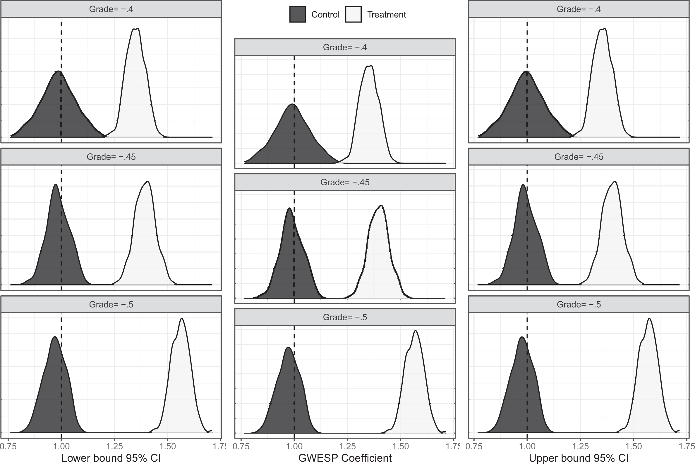
Effect of scaling on
Also of note are the confidence intervals in each simulation. Every confidence interval is narrow, and none of the confidence intervals in any of the treatment conditions contained the true GWESP (geometrically weighted edgewise shared partnerships) coefficient of 1. This result illustrates that scaling can pose problems for ERGM inference even when resampling is possible because confidence intervals rescale alongside ERGM coefficients. These results illustrate that the consequences of scaling for conclusions about effect size can be substantial. Even though even though ReceiverGrade and GWESP are uncorrelated, the bias in the bias in estimated coefficients is sizable in every treatment condition. We therefore caution researchers against relying on coefficients and exponentiated coefficients to interpret effect size in ERGM applications.
Simulation of Differences in Coefficients
We now consider the effect of scaling on the difference in coefficients using a simulation based on the Faux Mesa High network data. The Faux Mesa Network is an undirected network of 205 students and 203 ties. We first estimated an ERGM predicting ties as a function of students’ sex and GWESP (fixed decay term equal to 0.3). Next, we simulated a confounding or mediating edge covariate M to be correlated with

where the coefficients for
At each replication, we fit two ERGMs to the simulated network data to calculate the naive difference in coefficients. The first ERGM predicted ties as a function of the number of edges and GWESP; the second ERGM included M. Because
Figure 2 summarizes simulation results. When there are low amounts of residual variation, the naive difference in coefficients is small in value and close to 0. Here, the mean naive difference in coefficients is 0.03 despite the mean true difference being substantial in size at 0.17. In other words, the estimated difference in coefficients is 17 percent of the size of the true difference in coefficients. The naive difference in coefficients also provides the incorrect sign in 26 percent of cases. Increasing residual variation increases the discrepancy between the true and naive difference in coefficients. For instance, when
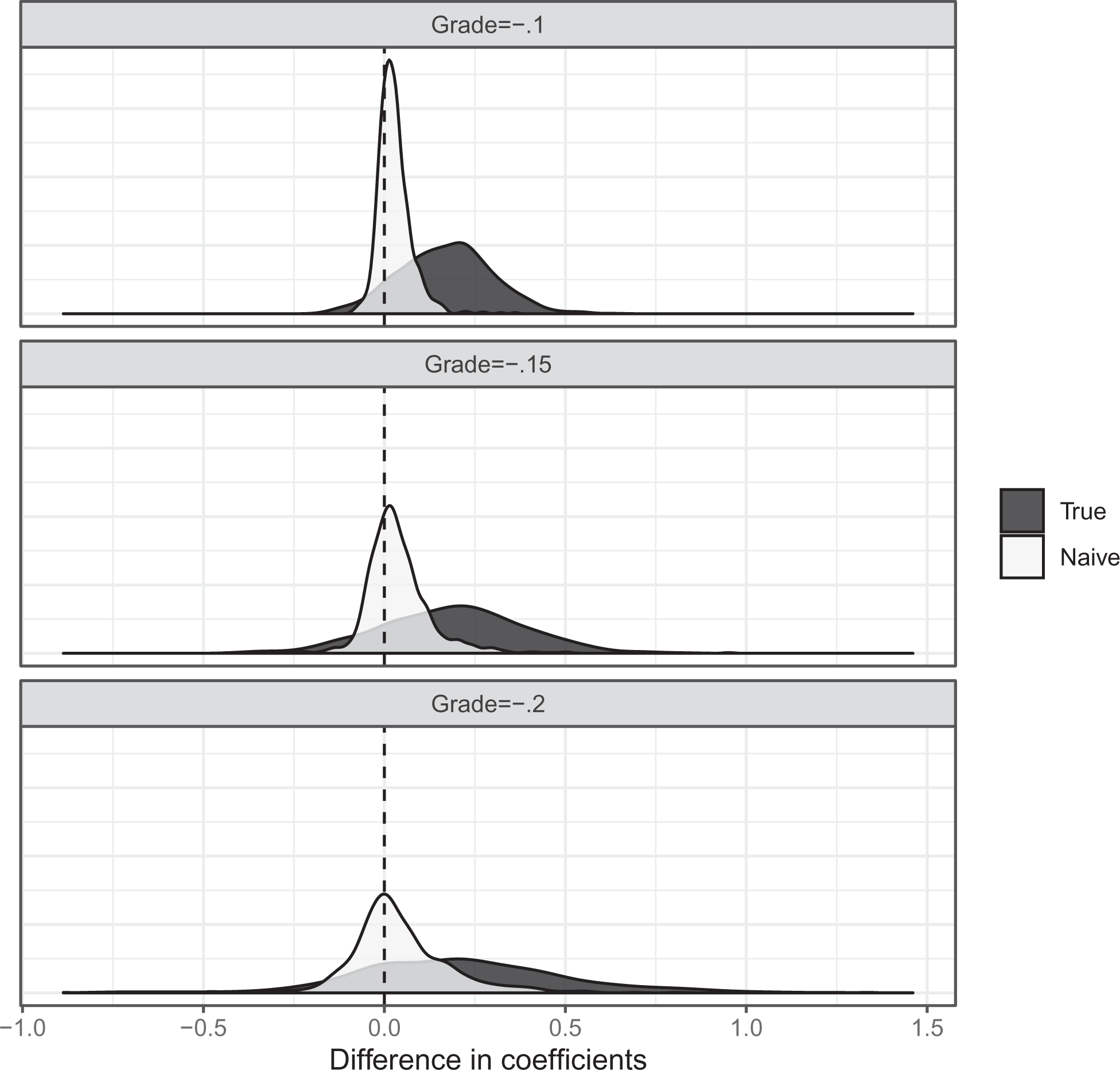
Effect of scaling on difference in coefficients. Note:
Simulation of Interaction Coefficients
We now return to the Faux Dixon network data to examine the impact of scaling on interaction coefficients. We first fit an ERGM to the Faux Dixon High network with the form:
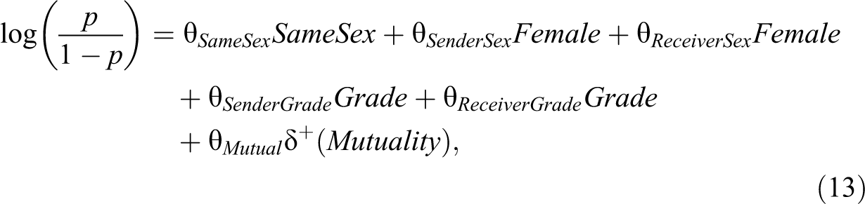
where the
ERGM of Friendships in Faux Dixon High.
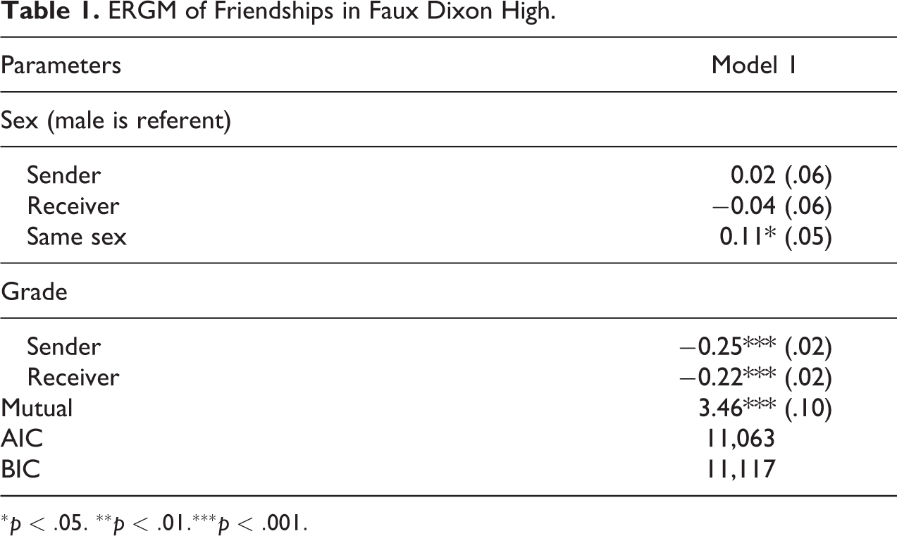
Figure 3 summarizes the simulation results. In the control condition, the simulated values of
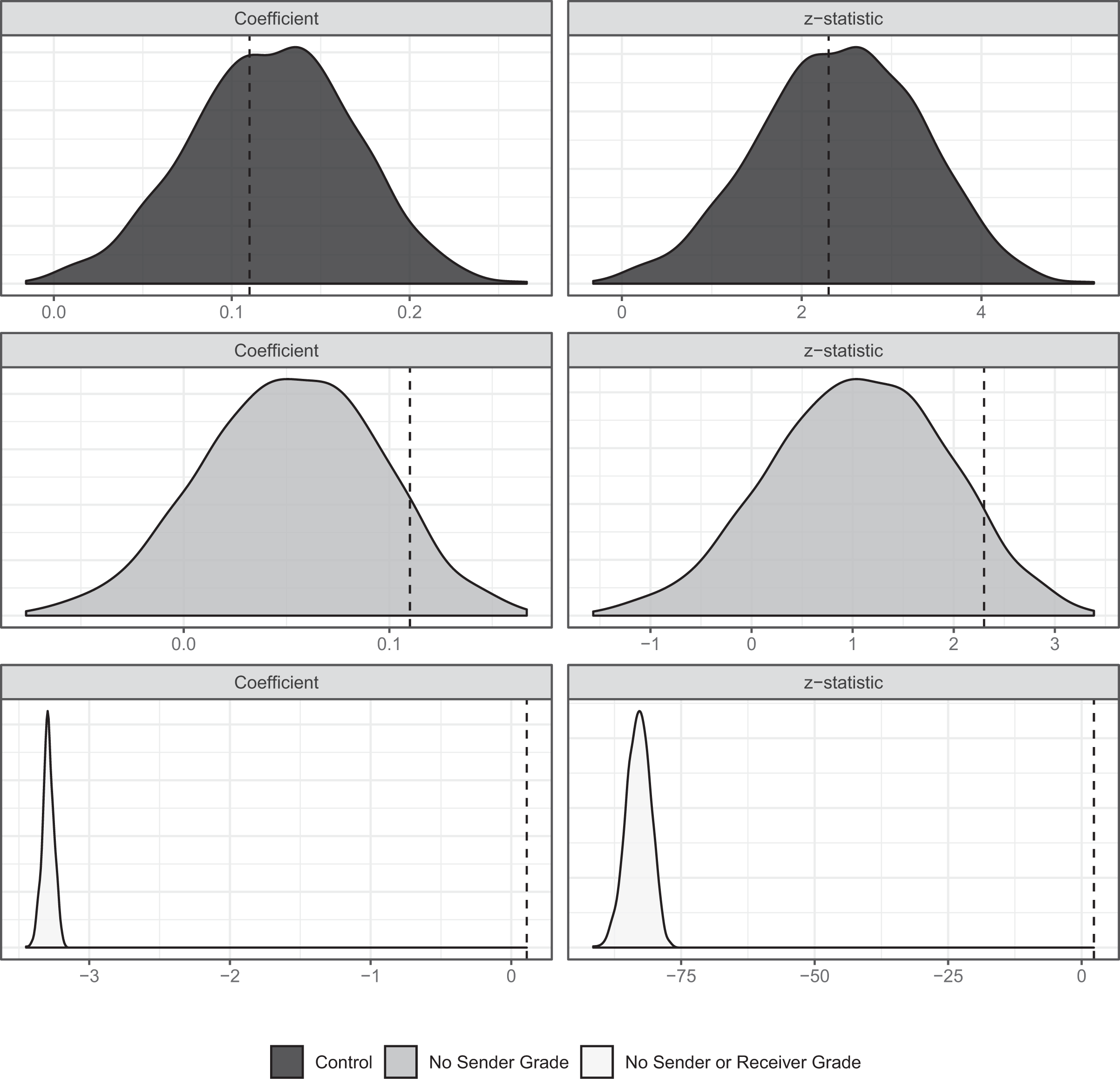
Effect of scaling on
Summary of Simulation Results
Simulation results illustrate that residual variation and scaling have important consequences for interpreting effect sizes, assessing differences in effects between models, and interpreting and testing interactions. When residual variation is present, ERGM coefficients are a biased measure of effect size, and this bias can be substantial under realistic circumstances. Coefficients also frequently rescale between models, suppressing differences in effects and potentially altering conclusions about confounding and mediation. Interaction coefficients and their z statistics are also often biased in the simulations, frequently yielding the incorrect sign. Collectively, these results illustrate that realistic amounts of residual variation can have large consequences for ERGM inference. We now introduce methods for addressing scaling in ERGM.
Methods for Handling Scaling
Simulation results reveal that realistic amounts of scaling can have large consequences for ERGM inference. Because we rarely have observational measures of all relevant variables, it is likely that these problems are common in practice. How should this issue be overcome in applied research? While a number of studies have proposed solutions for addressing scaling and rescaling in GLM (generalized linear models), their extension to statistical network models is problematic. Most solutions that circulate the literature on GLM assume independent and identically distributed observations—an assumption violated by network data. For instance, one popular method for comparing coefficients between models is to first regress the confounding variable of interest on the remaining predictor variables and then standardize the focal variable using the residual from this regression (Breen et al. 2013; Karlson et al. 2012; Mackinnon et al. 2007). Since residuals are biased by nonindependence and endogeneity, this method cannot be used in dyadic dependence ERGMs. Likewise, a common strategy for testing interactions is to estimate separate regressions for each group and use likelihood ratio tests to assess the equivalence of coefficients between groups (Allison 1999). However, because network data are interdependent, splitting the data into separate models will fundamentally damage the representation of network structure with potentially impactful consequences.
We propose using a marginal effects framework to overcome problems related to scaling in ERGM. While ERGM coefficients can only be identified to a scale, scaling has no effect on predicted tie probabilities (see Online Appendix A, which can be found at http://smr.sagepub.com/supplemental/). Moreover, because marginal effects are obtained in postestimation, the only necessary independence assumption is that the ERGM is estimated at the correct level of independence, which is an assumption implicit in all ERGMs (Koskinen and Daraganova 2013). The framework integrates methods that have been recently proposed for GLM (Long and Mustillo 2018; Mize, Doan, and Long, 2019; Mood 2010) but can be extended to ERGM due to their relaxed independence assumptions. The framework is flexible and can be easily applied across ERGM specifications and applications. We focus here on the average marginal effect (AME), though all methods can be applied to any marginal effect variant, including partial effects (see Wooldridge, 2002), marginal effects at means (Agresti 2002; Long 1997), or marginal effects at representative values (Long and Mustillo 2018; Mize et al. 2019). 13
Interpreting Effect Sizes
Marginal effects are based on the derivative of the slope at a particular point in the cumulative distribution function (equation 3). The marginal effect for a variable is the expected increase in tie probability when the variable increases by 1. For a continuous variable, we define the marginal effect with respect to a variable X as its partial derivative,

For binary variables, the partial derivative is equivalent to the difference in tie probabilities when X changes from 0 to 1. The superscript
The AME of a variable is its mean marginal effect. Formally, we calculate the AME as:

where n is the number of dyads in the ERGM sample space. The AME expresses the average change in expectation given a one-unit increase in X. It can be calculated on either the scale of the ERGM linear component or the scale of tie probabilities. Standard errors are obtained with the Delta method (see Agresti 2002). 14 The Delta method standard error provides a z statistic equal to the coefficient z statistic for noninteraction coefficients. AMEs therefore do not affect conclusions regarding the significance, direction, or relative size of effects within a model for non-interaction terms. 15
An appealing property of the AME is that it has an intuitive interpretation. Suppose that we are examining the effect of age on friendship networks and we obtain an AME of 0.005 (calculated on the scale of tie probabilities) and a coefficient of 2. A one-unit increase in the coefficient for age would correspond to an exp(2) = 7.38 increase in the estimated odds of a friendship. However, because of scaling, we cannot be sure that the estimated odds ratio is the true odds ratio. Moreover, because odds ratios are ratios, the substantive change in tie probability varies multiplicatively for each unit increase in age. Alternatively, we can interpret the AME equivalently regardless of the value of age or amount of scaling: A one-year increase in age correlates with an average 0.005 increase in tie probability. This interpretation is more intuitive and often more immediately relevant to research interests than odds ratios. Moreover, because AMEs do not rescale between models or groups, they provide a basis for drawing cross-model comparisons and for evaluating interaction effects. We now introduce these methods for ERGM.
Testing Differences between Models
As described above, we cannot attribute the difference in coefficients to confounding or mediation. Comparisons of coefficient significance are also problematic as the difference between significant and insignificant is not, in itself, statistically significant (Bollen and Stine 1990; Gelman and Stern 2006). To assess the change in effect size, we calculate the difference in the AME between models:

Because AMEs are robust to scaling but are still affected by omitted correlates, AMEs only change in size when a confounding variable is excluded or included. Differences in AMEs can therefore be attributed to substantively relevant differences in effects.
To determine whether the change in AME is statistically significant, we use a Wald test with test statistic:

where the denominator is the standard error for the difference in AMEs. Rejecting the null hypothesis means that there is a statistically significant difference in AME between models.
To calculate the standard error for the difference in AMEs, we require the variance estimates for both AMEs and the cross-model covariance between AMEs. We obtain the cross-model covariance using seemingly unrelated estimation (Mize et al. 2019; Weesie 1999). Suppose

where
A desirable property of equation (17) is that it reduces to a Sobel test (see Sobel 1986) in large-sample linear models (see Online Appendix D, which can be found at http://smr.sagepub.com/supplemental/).
16
Under standard assumptions for mediation analysis (see Mackinnon 2008:53-55), we can use this method as a formal test of mediation. If we are conducting mediation analysis, the difference in AMEs is the indirect effect, or the average change in tie probability indirectly attributable to X through a mediating pathway. We can interpret
We can assess the extent of mediation by calculating how much of the total effect is explained by controlling for the mediator. The percent mediated is

The percent mediated is a useful quantity when the goal is to summarize the degree of confounding by including a correlated variable. However, the quantity may be misleadingly large if the total effect is small. Researchers will often wish to interpret the percent mediated with respect to the total and indirect effects.
Simulation
Because there is no baseline method for comparing coefficients between models in ERGM, it is useful to demonstrate the validity of the proposed test under conditions of residual variation. The following simulation uses the Faux Desert High network, which is a simulated friendship network based on one rural Southwest high school in the AddHealth data collection. The network is undirected
17
with 107 students and 439 friendship ties. We first estimated an ERGM to the network of the form
To conduct the simulation, we simulated random networks using the above model, but we included a random nodal-level covariate with a mean of 0 and a standard deviation 1 to manipulate residual variation. The random variable was uncorrelated with any other predictor. Its coefficient could obtain three possible values of 0.5, 1, and 1.5. We fit four ERGMs to each network and assessed the difference in AMEs for each matched pair. The first pair of ERGMs was estimated with and without
Figure 4 plots the differences between the true and estimated values of

Difference in true and estimated
Testing Interaction Effects
As demonstrated in simulation analyses, excluding as few as two uncorrelated explanatory variables can reverse the sign of ERGM interaction coefficients. We now show how marginal effects can be used to interpret and test interaction effects in ERGM. Moderation exists when the effect of a variable varies when a second variable changes in value. We measure the interaction effect using the second difference in AMEs (Long and Mustillo 2018). We define the AME for a level of an interaction as

If g is binary, the only second difference for the interaction is when g changes from 0 to 1. If g is continuous, we can specify the values of g to be any values in the data set. We can also set g to representative values or summary statistics, such as the mean plus or minus one standard deviation.
We interpret the second difference as the increase/decrease in AME when g changes in value. Say that we are interested in assessing the effect of sex homophily in a friendship network. The AME of interest is a binary indicator variable for female students. Let the AME for male alters be 0.001 and the AME for female alters be 0.004. The second difference would be 0.003, indicating that the effect of being female on tie probabilities increases by 0.003 when an alter is female instead of male, reflecting a preference for same sex friendships. We assess significance using a Wald test with the following test statistic:

where the denominator is the standard error for the second difference. As before, we can use the Delta method to estimate the AME covariance matrix.
When g has a large number of unique values, it may be difficult to succinctly summarize the impact of an interaction using second differences. One way to do so is to compute the second difference when g changes from its smallest value to its maximum, which will provide insight to the overall change in the interaction effect. In other cases, researchers may simply want to report the average interaction effect or the average second difference. We first calculate the second differences for all k in increasing order and then take the mean second difference:

where Nk is the number of unique values in g. We can interpret
Because marginal effects are robust to scaling, we can also compare second differences between models. For instance, if we are studying a school friendship network, we may be interested in evaluating whether triadic closure explains the effect of sex homophily. We estimate two ERGMs, one that includes sex homophily, and one that includes both sex homophily and triangles. We would then compute the second difference for sex homophily in each model and use equation (17) to test their equivalence, replacing the AMEs with second differences.
Summary
The marginal effects framework outlined above provides a strategy to overcome problems of scaling in ERGM. Because it is typically impossible to determine that there are no omitted variables in a model, we recommend that researchers use these methods to interpret effect size, test for and interpret interaction effects, and to compare effects between models. These methods are available for use via the opensource software package ergMargins for R (Duxbury 2019), available through the Comprehensive R Archive Network repository and as a part of the xergm suite of packages. We now apply these methods in an empirical application reexamining the role of selective mixing and triadic closure in a large AddHealth school friendship network.
Empirical Application: Revisiting Birds of a Feather or Friend of a Friend?
To demonstrate how these methods can be used to correct for scaling, we examine the relationship between selective mixing and triad counts in one large AddHealth friendship network. An empirical regularity in social networks is high levels of clustering (Newman 2010; Watts and Strogatz 1998). Observed levels of clustering in social networks are typically attributed to two underlying processes: selective mixing (preferential attachment to similar alters) and triadic closure. Goodreau et al. (2009) sought to disentangle these two processes using ERGM on a pooled sample of 59 school networks from the AddHealth data set. Based on comparisons of homophily coefficients between models, they found that (1) triadic closure explains much of the effect of selective mixing, (2) that selective mixing promotes triadic closure, and (3) that there is little relationship between students’ nodal attributes and triad closure, with the exception of female students’ tendency to be embedded in triangles.
However, because coefficients are only identified to a scale in most ERGM applications, we are unable to compare homophily coefficients between models or interpret them as evidence of a homophily effect. We now revisit this research question in a replication analysis of the largest AddHealth in-school network in Goodreau et al.’s (2009) sample. The network contains friendship nominations between 2,209 7th and 12th graders (school ID: 44 in the supplementary tables to Goodreau et al. 2009). While the in-school network is directed, we follow Goodreau et al.’s (2009) inclusion criteria and only examine the 1,893 mutual ties between students. Our model specification is, for the most part, identical to the original study. The only difference is that we include Native American students in the “other” racial category, instead of as an independent group. Nodal covariates or “sociality” terms include students’ race (whites are referent), sex (males are referent), and grade (7th grade is referent). Each sociality term is treated as a categorical variable, with missing values controlled for as a discrete category. Selective mixing is measured by including homophily (matched attribute) interactions for each nodal covariate. Triadic closure is measured with a GWESP term using a fixed decay parameter of 0.25. Consistent with Goodreau et al. (2009), we estimated three models. The first is a dyad independence model including only exogenous attributes. The second is a curved ERGM including only the GWESP parameter. The third is a fully specified model including all variables.
Table 2 presents results (Panel A). While we were unable to perfectly replicate Goodreau et al.’s (2009) models, the substantive results are mostly consistent in terms of direction, relative coefficient size, and differences in coefficients between models. 19 In model 1, female students have higher tie probabilities as compared to male students. Black and Asian students have higher tie probabilities than whites, while Latino students have lower tie probabilities. Naive interpretations of selective mixing coefficients also suggest that there is a preference for sex, race, and grade homophily across categories. Model 2 includes only GWESP and an edges term. The positive coefficient indicates that triadic closure increases the probability of friendship formation. Model 3 presents full model results. The percent change in coefficients indicates that most coefficients decline in size in the full model, with the exception of the black sociality coefficient. Consistent with Goodreau et al. (2009), the change in coefficient size is also quite large, with most coefficients declining by more than 20 percent. If scaling were not a problem, these results would indeed imply confounding. We now turn to AMEs to interpret effect size, interaction effects, and differences in effects between models.
ERGM of Friendships in Large AddHealth School Network.
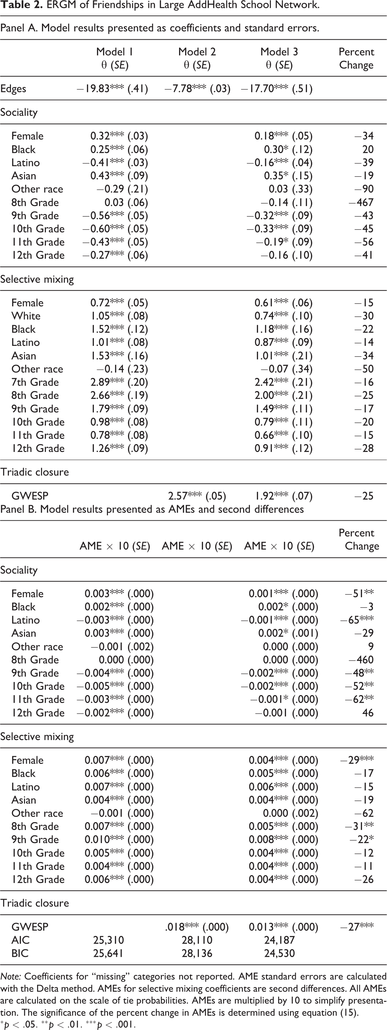
Note: Coefficients for “missing” categories not reported. AME standard errors are calculated with the Delta method. AMEs for selective mixing coefficients are second differences. All AMEs are calculated on the scale of tie probabilities. AMEs are multiplied by 10 to simplify presentation. The significance of the percent change in AMEs is determined using equation (15).
Panel B in Table 2 presents results as AMEs and second differences. A focus on AMEs reveals that the sociality effect sizes are relatively small. For instance, the AME for female students is 0.0003 in model 1, indicating that female students are only, on average, 0.03 percent more likely to be part of a mutual friendship than male students. Based on these averages, we would expect that an Asian female student in seventh grade would only be 0.11 percent more likely—one tenth of one percent—to form a mutual friendship than a white male student in 10th grade (0.0003 + 0.0003 − (−0.0005) = 0.0011). By comparison, the AME for GWESP is 0.002 in model 2, indicating that a one-unit increase raises the tie probability by 0.0018 (0.18 percent increase), with diminishing returns. In other words, closing a single triangle yields a greater difference in tie probabilities than the absolute difference in tie probabilities between the demographic most likely to forge a tie (seventh grade Asian female students) compared to the least likely demographic (10th grade White male students). This stands in contrast to the substantive impact implied by the sociality coefficients, which appear, at least intuitively, to have noteworthy effect sizes.
We now assess the interaction effect for homophily terms in model 3. Results for the direction and significance of second differences are consistent with those for interaction coefficients, indicating that scaling is not problematizing conclusions about the positive influence of homophily. However, it is also clear that interaction coefficients imply misleading conclusions about interaction effect size. If we were to interpret homophily coefficients as odds ratios, for instance, we would conclude that eighth grade homophily increases the odds of friendship seven times over (exp(2.00) = 7.39). Likewise, we would conclude that same sex friendships increase the odds of friendship by 84 percent (exp(0.61) = 1.84). Figure 5 makes clear that the differences in interaction effect sizes are not that large. Instead, the interaction effect for eighth grade friendships is approximately equal to the interaction effect for female friendships. In fact, the largest second difference is for same grade friendships among ninth graders, which has a smaller coefficient than 8th grade homophily. We arrive at a similar result for racial homophily. Although the homophily coefficient is largest for black students, the homophily interaction effect is greatest for Latinos. These results illustrate that even in cases where scaling does not problematize conclusions about the significance and direction of interaction coefficients, it can still alter conclusions about the relative and overall importance of interaction effects.
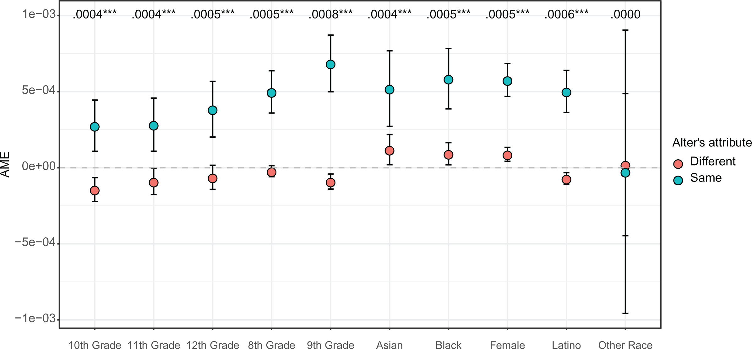
Average marginal effects for homophily terms. Note: X axis is students’ attributes. Bands are 95 percent confidence intervals. Second differences are printed at the top of the plot.
Our final goal is to examine differences in effects between models. Although the percent change in AMEs is similar to the percent change in coefficients for some covariates, it is quite different for others. For instance, while the coefficient for black students increases by 20 percent, the AME does not change, indicating that the increase in coefficient size is entirely a result of scaling rather than a suppressing effect. This is particularly relevant for 12th graders. Even though the coefficient for 12th graders changes from significant to insignificant, a test of the difference in AMEs reveals that this change in significance is not itself statistically significant.
Moreover, even though most AMEs change by more than 10 percent between models, the difference in effects is only significant for 9 of the 21 model terms. Consequently, despite the relative change in coefficient size being fairly large in many cases, the conclusion of confounding is not supported for most covariates. In fact, while each second difference changes by more than 15 percent between models, the difference in second difference is only significant for 3 of the 10 interactions. Notably, there is no significant change in any of the racial homophily second differences. This contrasts with the differences in racial homophily coefficients, which decline by 15 percent to 35 percent between models. These results suggest that there is little systematic relationship between selective mixing and triadic closure in the school 44 network.
An interesting and unique result that arises from comparisons of AMEs is that the differences in AMEs are greater for nodal covariates than for homophily covariates (Table 3). Five of the 10 differences in sociality AMEs are statistically significant. For instance, the AME for female students declines by 51 percent between models. The direct and indirect effects for sex are both 0.0001. This means that, compared to male students, female students have a 0.0001 higher probability of forming friendship ties because of their gender (direct effect). The indirect effect reflects that being female is also
Mediation Analysis for Sociality AMEs with GWESP as the Mediator.
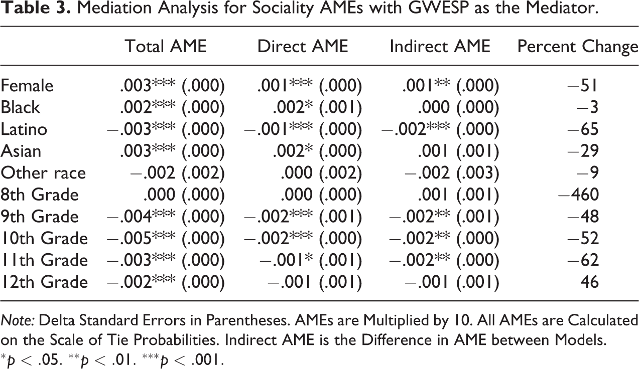
Note: Delta Standard Errors in Parentheses. AMEs are Multiplied by 10. All AMEs are Calculated on the Scale of Tie Probabilities. Indirect AME is the Difference in AME between Models.
Similarly, accounting for triadic closure explains a substantial portion of the effects of being in 9th, 10th, and 11th grade. The percent mediated for each of these variables ranges from 45 percent to 60 percent. This result suggests that part of the reason that students’ grade is predictive of tie probabilities is because it affects triangle counts; that is, students in 9th, 10th, and 11th grade tend to be embedded in a greater number of triangles as compared to students in 7th grade. The AME for Latinos also declines by 65 percent after controlling for GWESP. Because the percent mediated for sociality AMEs are on average larger than for selective mixing terms, these results suggest that triangle counts explain a greater share of the effect of sociality than they do of selective mixing.
A replication of Goodreau et al. (2009) reveals how scaling can alter conclusions in ERGM applications. While findings regarding the direction and significance of sociality, triad closure, and selective mixing effects were supported, conclusions regarding the substantive impact of these covariates and those related to indirect effects were problematized. Particularly, sociality terms appear to have small effect sizes when we correct for scaling. We further found that scaling affected the relative size of homophily coefficients, altering conclusions regarding the relative impact of some types of selective mixing. Scaling also led to increases in homophily coefficient size that were not reflected in the homophily effects, causing homophily coefficients to overstate the substantive importance of some types of selective mixing, like eighth grade homophily. Finally, a reanalysis of the differences in effects between models shows how scaling can alter conclusions about confounding and indirect pathways. Selective mixing only appears to affect triangle counts in the minority of cases. Further, sociality terms have greater impact on triadic closure than selective mixing, which is not reflected in comparisons of naive coefficients.
Discussion
Residual variation can have large consequences for ERGM inference. The equality of coefficients cannot be compared between models or groups in any scenario where coefficients are scaled nor can coefficients be interpreted as effect sizes. Because the assumption of no omitted variables is difficult to verify, we can rarely outrule the possibility of residual variation and scaling in practice. This study outlined these issues and proposed resolutions using marginal effects. The methods are robust to scaling and can be flexibly applied across ERGM specifications. These methods were further extended to develop formal tests of mediation and moderation, which have yet to be introduced for statistical network analysis. Collectively, the methods provide a flexible framework for interpreting effect sizes and conducting process analysis in research using statistical network methods.
While the methodological discussion here focused on ERGM, the same issues can also affect inference in other statistical network models that can be represented as logit models. Stochastic actor-oriented models, for instance, use a multinomial logistic regression to model network and behavioral change (Snijders 2001). Generalizations of ERGM map weighted edge data to a binary ERGM reference distribution (Desmarais and Cranmer 2012; Krivitsky 2012), and temporal ERGM reduces to an ERGM with block structure (Hanneke et al. 2010). Likewise, relational event models are often estimated as a logistic regression (Butts 2008). Because the proposed methods rely on postestimation, they can be used to overcome scaling in any of these models. The methods can therefore be flexibly applied in a variety of social network research to assess interaction effects and indirect pathways. They can also be applied in research using frailty ERGM (see Box-Steffensmeier et al. 2018) to address omitted confounding variables and rescaling simultaneously.
A further implication of our results is that meta-regressions of statistical network model output may be affected by scaling. Researchers often use meta-regression to combine output from multiple ERGMs, where the meta-coefficient is a weighted or unweighted average of the lower-level coefficients. The averages of these coefficients can be confounded with residual variation. Because each lower-level ERGM is identified to a unique scale (
In sum, ERGM results can be affected by scaling, which often arises when there is residual variation in an empirical model. Because we cannot test for all possible sources of residual variation (i.e., omitted variables), it is extremely difficult to rule out the possibility of scaling in practice. A methodological framework was introduced to overcome problems of scaling in ERGM. Formal tests were also developed to test the equivalence of marginal effects between models and groups. These methods can be applied to conduct mediation and moderation analysis in ERGM and related statistical network models. As such, they introduce a new methodological toolkit that can be used to assess the significance and effect of interactions and indirect pathways in statistical network analysis.
Supplemental Material
Supplemental Material, sj-docx-1-smr-10.1177_0049124120986178 - The Problem of Scaling in Exponential Random Graph Models
Supplemental Material, sj-docx-1-smr-10.1177_0049124120986178 for The Problem of Scaling in Exponential Random Graph Models by Scott W. Duxbury in Sociological Methods & Research
Footnotes
Acknowledgments
I thank David Melamed, Jacob Young, David Schaefer, Skyler Cranmer, and Carter Butts for helpful comments and conversations at various stages of this project.
Declaration of Conflicting Interests
The author(s) declared no potential conflicts of interest with respect to the research, authorship, and/or publication of this article.
Funding
The author(s) received no financial support for the research, authorship, and/or publication of this article.

Supplemental Material
The supplemental material for this article is available online.
Notes
References
Supplementary Material
Please find the following supplemental material available below.
For Open Access articles published under a Creative Commons License, all supplemental material carries the same license as the article it is associated with.
For non-Open Access articles published, all supplemental material carries a non-exclusive license, and permission requests for re-use of supplemental material or any part of supplemental material shall be sent directly to the copyright owner as specified in the copyright notice associated with the article.
