
Abstract
The standard multilevel regressions that are widely used in neighborhood research typically ignore potential between-neighborhood correlations due to underlying spatial processes, and hence they produce inappropriate inferences about neighborhood effects. In contrast, spatial models make estimations and predictions across areas by explicitly modeling the spatial correlations among observations in different locations. A better understanding of the strengths and limitations of spatial models as compared with the standard multilevel model is needed to improve the research on neighborhood and spatial effects. This research systematically compares model estimations and predictions for binary outcomes between (distance- and lattice-based) spatial and the standard multilevel models in the presence of both within- and between-neighborhood correlations, through simulations. Results from simulation analysis reveal that the standard multilevel and spatial models produce similar estimates of fixed effects but different estimates of random effects variances. Both the standard multilevel and pure spatial models tend to overestimate the corresponding random effects variances compared with hybrid models when both nonspatial within-neighborhood and spatial between-neighborhood effects exist. Spatial models also outperform the standard multilevel model by a narrow margin in case of fully out-of-sample predictions. Distance-based spatial models provide additional spatial information and have stronger predictive power than lattice-based models under certain circumstances. These merits of spatial modeling are exhibited in an empirical analysis of the child mortality data from 1880 Newark, New Jersey.
1. Introduction
Multilevel regression analysis is one of the most widely used methods in the research of neighborhood effects on individual outcomes (Dietz 2002; Diez-Roux 2000; DiPrete and Forristal 1994). A standard multilevel model helps correct for within-neighborhood correlation among individual observations and thus adjusts for standard errors, resulting in efficient estimates for individual- and neighborhood-level predictors (Diggle et al. 2002). It also allows an assessment of within- and between-neighborhood variations (Snijders and Bosker 1994) as well as how individual- and neighborhood-level predictors contribute to these variations (Diez-Roux 2000). Nevertheless, the standard multilevel models typically ignore potential between-neighborhood correlations due to spatial diffusion processes, for example, and they assume independent observations in one neighborhood from those in another neighborhood, which may lead to the overstatement of the statistical significance of neighborhood effects (Chaix, Merlo, and Chauvin 2005).
Figure 1(a) illustrates a hypothetical example of the assumption of within-neighborhood correlation within the standard multilevel model. Each cell in the grid represents a neighborhood and its shading indicates the average level (from low to high as indicated by darker shades) of a certain individual outcome shared by the observations from that neighborhood. Within a neighborhood, each observation’s outcome deviates around the neighborhood’s mean. Neighborhood mean levels of a given outcome vary from one to another, resulting in more similar outcomes among the observations from the same neighborhood than those from different neighborhoods (depicted as different shades across cells in Figure 1[a]). The seemingly random distribution of mean outcomes at the neighborhood level across the entire study area reflects the assumption of between-neighborhood independence. That is, the mean outcome is no more similar between two adjacent neighborhoods than between two neighborhoods far away from each other.

Hypothetical examples of multilevel (a) and spatial (b) models.
In reality, however, between-neighborhood correlations may exist as a function of the distance between two nearby neighborhoods, as stated in Tobler’s First Law of Geography: “Everything is related to everything else, but near things are more related than distant things” (1970:236). First, a neighborhood’s socioeconomic and political resources are likely to be linked to those in adjacent neighborhoods within a larger citywide system (Logan and Molotch 1987), which may in turn lead to distinct spatial patterns of structural differentiation in individual outcomes across neighborhoods.
Second, social behavior and interaction are not necessary restricted within one’s immediate neighborhood, especially when the neighborhood boundaries are defined in a way that does not coincide with one’s real-life experience, such as census geography and postal code (Flowerdew, Manley, and Sabel 2008; Guo and Bhat 2007; Riva et al. 2008; Tatalovich et al. 2006). Instead, they may transcend neighborhood boundaries and thus be affected by or consequential to what happens in nearby areas (Liu, Wall, and Hodges 2005; Sampson, Morenoff, and Gannon-Rowley 2002). For example, collective efficacy in a neighborhood has been found to benefit residents living in adjacent neighborhoods (Sampson, Morenoff, and Earls 1999), while spatial proximity to poverty and violent crimes in adjacent neighborhoods has been associated with out-migration from current neighborhood (Morenoff and Sampson 1997).
Third, a spatial diffusion process may operate either within a city-wide system or even on a much larger geographic scale such that information, knowledge, techniques, innovations, products, languages, and diseases are likely to spread from one place to another. For instance, drawing on locational information for the incidence of homicide and participants’ residences, Cohen and Tita (1999) found a spatial spread of homicides from gang youth in one census tract to non-gang youth across neighboring tracts in the city of Pittsburgh during the period 1991 to 1995. On an even greater geographic scale, Hedström (1994) examined the growth of 16,911 trade unions that were distributed over districts across Sweden during the period 1890 to 1940. He found a significant association of union formations in a district with union activities, weighted by distance, in other districts. In short, exposure to social and environmental circumstances in one neighborhood can be correlated with those in another.
Spatial models have been developed to make estimations and predictions about space by explicitly modeling the spatial correlations among observations in different locations (Diggle, Tawn, and Moyeed 1998). Two of the key goals of spatial analysis are (1) to estimate the spatial distribution of an outcome of interest across the study area based on observations at a discrete set of locations and (2) to make predictions at a new location (Diggle, Ribeiro, and Christensen 2003). These model estimations and predictions typically involve certain stochastic assumptions about distance-based correlations among observations at known locations and unknown values at prediction locations. In addition to examining spatial distribution, spatial models also allow researchers to investigate associations between individual- and neighborhood-level predictors and outcomes of interest while adjusting for nonindependent observations (Chaix et al. 2005; Dietz 2002).
Figure 1(b) illustrates a hypothetical example of the assumption of the distance-decay correlation across neighborhoods in a spatial model. In addition to within-neighborhood correlation (as indicated by cells of different shades), a spatial model assumes that the strength of correlation between two locations declines as the distance between them increases, resulting in similar mean levels of outcomes among nearby neighborhoods and hence clusters of neighborhoods with similar mean outcomes (as indicated by the color gradient across the cells in Figure 1[b]).
Alternatively, spatial correlations across neighborhoods can be incorporated into a standard multilevel model in a variety of different ways, including multiple membership relationships in which individuals are involved (Browne, Goldstein, and Rasbash 2001), a conditional autoregressive structure among nearby neighborhoods with extra place effects (Arcaya et al. 2012), and other forms of correlated spatial random effects (Browne and Goldstein 2010). In essence, these models take an approach similar to that proposed by Diggle and colleagues (1998)—that is, extending the standard multilevel model by allowing additional spatial correlations across the neighborhood boundaries.
Chaix and colleagues (2005) are among the first to compare the spatial approach with the standard multilevel approach for studying neighborhood effects on health. Through empirical analyses of healthcare utilization in France, they demonstrated that the standard multilevel model can fail to capture both measures of associations between neighborhood factors and residents’ outcomes and measures of unexplained variation in these outcomes across areas. However, it remains unclear whether these results are valid only for these two specific data sources or whether they can be generalized to other research settings. Moreover, they did not provide a thorough comparison of model performance in terms of both model estimation and prediction between spatial and standard multilevel models through a formal approach such as simulation analysis (Burton et al. 2006).
While researchers have become increasingly interested in the spatial dynamics beyond simple neighborhood-level variation (Dietz 2002; Logan, Zhang, and Xu 2010; Sampson et al. 2002), the potential utility of spatial models in neighborhood studies remains underappreciated despite the recent advancements in spatial techniques and increased availability of spatial data. Thus, a better understanding of the strengths and weaknesses of spatial models as compared with the standard multilevel model is urgently needed to provide methodological guidance for empirical studies to avoid erroneous statistical inferences and substantive conclusions. The main purpose of this paper is to assess the impact of disregarding extant spatial correlations across neighborhoods when studying neighborhood effects on individual outcomes. The focus here is on models of binary outcome using a logit link because of their increased prevalence and popularity in neighborhood and spatial studies. By systematically comparing model performance in estimation and prediction between spatial and the standard multilevel models in the presence of both within- and between-neighborhood correlations through simulation analyses, this study informs researchers about making cautious model choices whenever spatial information is available, in addition to standard multilevel data structures. Drawing upon a real life data set, this study also illustrates the application of the spatial approach in empirical research and further demonstrates its relative advantages compared with the standard multilevel approach.
2. Multilevel and Spatial Modeling
2.1. Standard Multilevel Model
Let
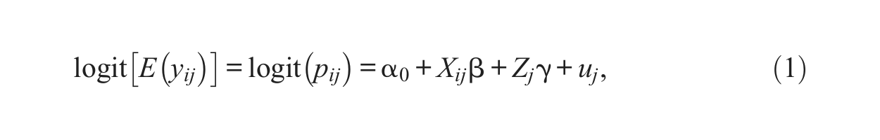
where
2.2. Pure Spatial Model
By contrast, a pure spatial model ignores within-neighborhood but incorporates between-neighborhood correlations in the following way:
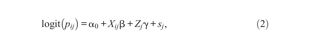
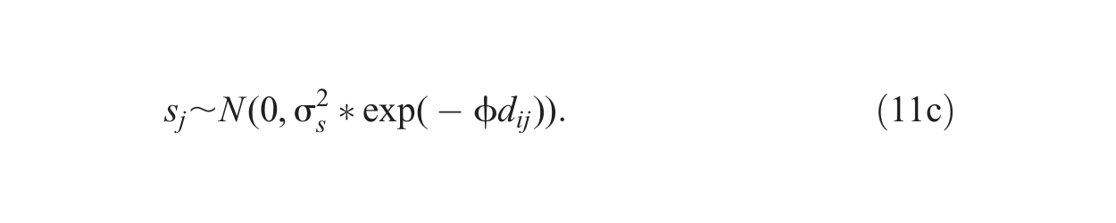
where distance-based correlation between neighborhoods is captured by the random effects
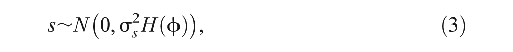
where

where ρ is typically chosen to be an isotropic function, which assumes that the correlation between two locations depends upon only their distance from each other, not on their relative orientations to each other. The so-called decay parameter
A common choice for the isotropic spatial correlation is the following exponential function because of its relatively simple form and hence relatively low computational cost as well as its wide availability in statistical packages:

Setting

Setting

and
2.3. Hybrid Model
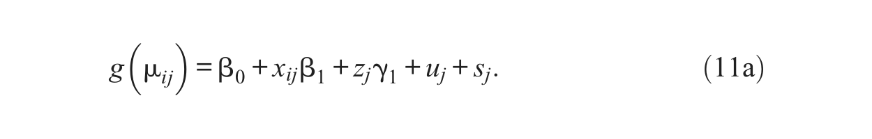
Combining the standard multilevel model and the pure spatial model above, Diggle and colleagues (1998) are among the first to develop a generalized linear spatial model as the following:

where uj and sj capture within- and between-neighborhood correlations as specified in equations (1) and (2), respectively. Details on parameter estimation and prediction using either maximum likelihood estimation or Bayesian inference can be founded in the work by Diggle and colleagues (1998; 2003).
Since then, other scholars have proposed alternative models that can simultaneously accommodate within- and between-neighborhood correlations in different ways. For example, Browne and Goldstein (2010:454) developed a modeling framework with correlated random effects that takes into account the possibility that “some pairs of clusters are more similar to each other than to other clusters” and meanwhile allows within-cluster correlations. Their modeling strategy takes essentially the same form specified in equation (8)—that is, a linear combination of a nonspatially structured correlation and a spatially structured correlation (i.e.,
Browne and Goldstein (2010) distinguish two ways to capture
The second way to capture
where
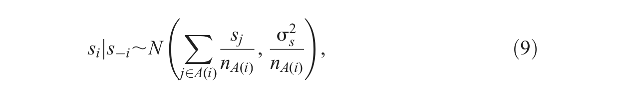
In their original example of county-level life expectancy, a continuous outcome, Acraya and colleagues (2012) formulated a multilevel-CAR model that simultaneously accounts for both place effects at the state level and space effects induced by each county’s adjacent counties ignoring state boundaries. With minor modifications of the hierarchical structure, their model can be adapted to the one specified in equation (8), where individuals are nested within neighborhoods (inducing place effects), neighborhood-level random effects are captured by uj, and between-neighborhood correlations (inducing space effects) are accounted for by a CAR specification for each neighborhood’s adjacent neighborhood units, as in equation (9).
The CAR model is closely related to the multiple-membership model described by Browne and colleagues (2001). Modifying their original example of count of male lip cancer in 56 regions of Scotland by considering a binary outcome for individuals nested within neighborhoods instead, their model can be written as follows:


where
The present study focuses on comparing four sets of models, including the standard multilevel model (as the reference model), the pure spatial model with distance-based correlations between neighborhoods, and two hybrid models with one using latticelike CAR structure and the other using more spatially explicit distance-based correlations as in the pure spatial model. Even though maximum likelihood–based estimates have been developed for both multilevel and spatial models, Bayesian inference is adopted in the present study for its relative merits. First, with the booming advancement in Markov chain Monte Carlo (MCMC) (Gilks, Richardson, and Spiefelhalter 1996) and data augmentation (Tanner and Wong 1987) algorithms in the recent decades, Bayesian analyses are highly flexible in expanding a standard multilevel model to accommodate more complex hierarchical (e.g., spatial) data structures without spending additional efforts in modifying existing estimation procedures. As a result, Bayesian inference has been widely applied in spatial statistics (e.g., Banerjee et al. 2004) and hence I made the choice in the present study to be consistent with the existing literature (Arcaya et al. 2012; Browne and Goldstein 2010; Browne et al. 2001; Chaix et al. 2005; Henderson, Shimakura, and Gorst 2002). Second, the extension from coefficient estimation to out-of-sample prediction can also be easily accomplished in a Bayesian framework by adding another hierarchical level—that is, by simulating predictive distributions that are conditional upon estimated posterior distributions of parameters. Thus, Bayesian predictions naturally incorporate the uncertainty inherent in parameter estimation from a sample of data, which often requires extra work to be appropriately addressed when using a maximum likelihood approach (Diggle and Ribeiro 2002).
3. Simulation Analysis
The simulation analysis here compares spatial and the standard multilevel models with respect to parameter estimation and prediction in the presence of both within- and between-neighborhood correlations. As the true data generation process and values of parameters are known a priori, which is never the case in any empirical study, the simulation analysis enables a direct assessment of the appropriateness and accuracy of a variety of models (Burton et al. 2006). To reduce the computational burden, the simulation analysis in this study focuses on the case of only one independent variable at the individual level and one independent variable at the neighborhood level. By varying the relative strengths of the within- and between-neighborhood correlations, the simulation study demonstrates the advantages and weaknesses of different spatial models in relation to the standard multilevel model that ignores spatial correlations, and hence provides guidance for model selection in empirical studies.
The gold standard K-fold cross-validation (Kohavi 1995) was employed in the simulation analysis. Simulation analyses that involve fitting the training data alone are susceptible to the issue of overfitting. The same model often reaches a relatively poor goodness of fit for an independent sample of the validation data from the same population as the training data. By partitioning a simulated data set into K subsets and rotationally leaving one subset out as validation data, the K-fold cross-validation allows a simple yet effective assessment of the predictive power across models—that is, it assesses to what extent the results of a model are generalizable to an independent data set, in addition to evaluating parameter estimation. Posterior predictive checks have been proposed as a goodness-of-fit test and diagnostic tool for discrete data regressions in Bayesian inference to overcome the difficulties associated with using other usual methods such as residual plots (Gelman et al. 2000). For each cross-validation data set, predictions are made for the validation observations with “missing” binary outcomes based on the model fitted to the training data. A comparison of the predicted values with the true values provides an easy yet straightforward way of assessing the accuracy of a predictive model in practice (i.e., out-of-sample prediction) while adjusting for uncertainty in estimating the model parameters.
Given that the assumption of distance-decay correlation underlies most spatial analyses and that the distance-based spatial correlation model remains something of an underdog in empirical research, it serves the “true” data generation mechanism in the present study. Taking exponential spatial correlation structure as an example, the entire simulation procedure can be summarized in the following steps:
An exponential spatial correlation structure is simulated using the geoR package (Ribeiro and Diggle 2001) in R (R Development Core Team 2012) with a mean 0, a partial sill
Neighborhood-level random effects are generated from a normal distribution with a mean 0 and a variance
A neighborhood-level predictor (i.e., neighborhood-level fixed effects), z, is sampled from a standard normal distribution across 64 neighborhoods. Within each neighborhood, an individual-level predictor (i.e., individual-level fixed effects), x, is also sampled from a standard normal distribution for 30 observations, resulting in a total number of 1,920 observations. The values of the two predictors are then multiplied by their associated regression parameters β and added together to obtain the linear combination of fixed effects for each observation.
For each observation, the values of fixed effects, neighborhood random effects, and spatial random effects are summed up to obtain the full linear combination of predictors as in the right-hand side of equation (8), which in turn is used to generate the binary outcome from a logistic distribution.
A fourfold cross-validation is constructed by randomly partitioning a simulated data set as described above into four mutually exclusive subsamples, each of which contains 480 observations. Each of the four subsamples is used in turn as the so-called validation data. That is, the outcome values of its 480 observations will be treated as unknown, while a model will be fitted to the other three subsamples with 1,440 observations, known as the training data. Predictions for the 480 observations in the validation data will be made based on the fitted models and compared with their true values to assess the model performance.

A simulation of spatial random effects with an exponential function (σs2 = 3,
To summarize, the mean response for the ith observation in the jth neighborhood was generated according to the following model with both within- and between-neighborhood correlations:

Throughout the simulations, the true values for the fixed effects parameters are kept as
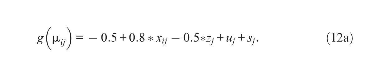


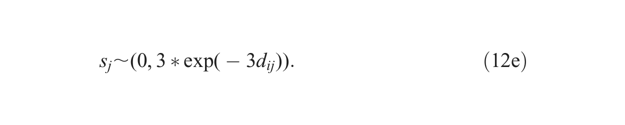
In order to mimic real data more closely, extra noise was added to the linear predictors in equation (12a) by making a random draw from N(0, 1). The seemingly large values of
Scenario 2 applies the same values of
The validation data set is constructed in two different ways. First, as is conventionally done, the 480 observations are randomly selected across the entire study area so that in each subsample of the fourfold cross-validation, each neighborhood is likely to have some observations in the validation data and in the training data. This approach allows model comparisons in terms of making predictions for “new” observations with different individual attributes but the same neighborhood attributes and spatial location information as those in the training data. Thereby, the first approach is hereinafter referred to as “partially out-of-sample” cross-validation.
Second, instead of randomly choosing individual observations, 16 neighborhoods are randomly selected for each subsample of the fourfold cross-validation. All the observations (480 in total) in these selected neighborhoods are assigned missing outcome values and treated as validation data. In contrast to the first approach, the second approach is focused on comparing the predictive power of “new” observations with not only individual but also neighborhood attributes and spatial locations that are different from those in the training data. Thus, the second approach is referred to as “fully out-of-sample” cross-validation.
For both partially and fully out-of-sample cross-validation, a total number of 100 data sets were simulated for each set of parameter values. Each data set was partitioned into four subsamples, resulting in 400 data sets in total for model fitting. Four models were fitted to each simulated data set and compared, including a standard multilevel model that adjusts for within-neighborhood correlation, a pure spatial model that adjusts for distance-based between-neighborhood correlation but ignores within-neighborhood correlation, and two hybrid models that adjust for both within- and between-neighborhood correlations. The first hybrid model accommodates the spatial correlation through lattice-based CAR distribution as specified in equation (9), and it is referred to as the hybrid CAR model. The second one models distance-based between-neighborhood correlation; it is thus the “true” model in the simulation analysis and is referred to as the hybrid spatial model. The standard multilevel model mainly serves as a benchmark for assessing the other three models.
Model estimation and prediction were carried out by using OpenBUGS version 3.2.2 (Lunn et al. 2009), an open-source software package for performing Bayesian inference using MCMC algorithms. To ensure model convergence, each model was fitted by initiating 2 MCMC chains with different starting values and letting each chain run for 60,000 iterations. Model convergence was monitored by graphically examining the trace plots of MCMC chains as well as computing the Gelman-Rubin statistic (Brooks and Gelman 1998; Gelman and Rubin 1992), a measure for assessing the convergence of multiple chains based on between- and within-chain variances. After discarding the first 30,000 iterations as the burn-in, each chain was then thinned by storing the sampled parameter values from every 50th iteration in order to reduce its autocorrelation, which resulted in a total number of 1,000 iterations from the two chains, from which the posterior distributions are summarized. Noninformative priors are adopted for all the unknown parameters, including a normal distribution N(0, 100) for the fixed effects (β), a uniform distribution U(0, 10) for the standard deviation of the random effects (
Several performance measures are adopted to evaluate parameter estimation from different models (Burton et al. 2006). Bias is assessed by the difference, calculated as a percentage of the true value, between the average estimate and the true value, known as the percentage bias (PB). Coverage is assessed by the proportion of times the true parameter value falls within the estimated 95% credible interval, known as the coverage rate (CR). Accuracy is assessed by the mean-squared error (MSE) which is a combined measure of bias and variability. The relative goodness of fit of a model was measured by the deviance information criterion (DIC) (Spiegelhalter et al. 2002), a hierarchical modeling generalization of the Akaike information criterion (AIC) widely used to compare non-nested regression models (Akaike 1974). A smaller value of the DIC indicates a better model fit to the data.
4. Simulation Results
This section first assesses model performance in terms of parameter estimation and prediction based on partially and fully out-of-sample cross-validation, and then it evaluates robustness against model misspecifications from fully out-of-sample cross-validation.
4.1. Partially Versus Fully Out-of-sample Cross-validation
Table 1 presents measures of parameter estimation from logit models fitted to data generated from a process in which spatial correlation follows an exponential distance-decay function. For partially out-of-sample analysis, only the results from Scenario 1 (i.e., strong spatial correlation and long effective range) are shown as those from other scenarios are largely similar. Under Scenario 1, the four models perform somewhat similarly with respect to the accuracy, precision, and efficiency of the estimation of the fixed effects (i.e.,
Performance Measures for Logit Models Fitted to 100 Simulated Data Sets with Fourfold Cross-validation

Note: TV = true value; AE = average estimate; PB = percentage bias; CR = coverage rate with 95% credible interval; MSE = mean squared error.
Exponential spatial correlation function.
Remarkable variations appear across the four different types of models in their estimation of the random effects variances. With respect to
In the case of fully out-of-sample cross-validation, the variation in parameter estimation across the four types of models is substantially reduced under Scenario 2 (weak spatial correlation and long effective range) and 3 (strong spatial correlation and short effective range). For example, the standard multilevel model has a smaller MSE for the estimate of
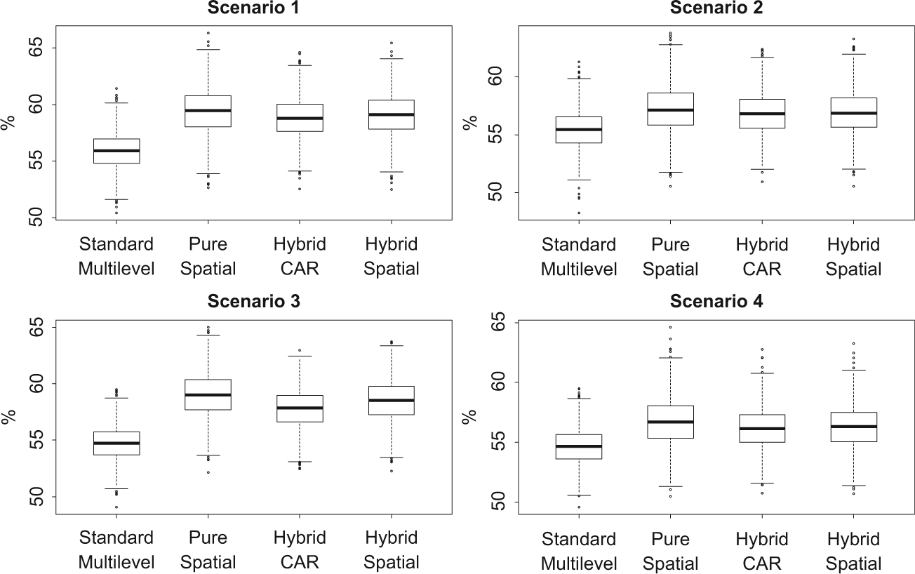
One difference between partially and fully out-of-sample cross-validation comes from predictions for new observations. Model comparison in terms of predictive power is based on the predictive match rate—that is, the percentage of correct predictions for the validation data whose true outcome values are known a priori but assigned as missing at the modeling stage. There is almost no difference in the predictive power across the four different types of models when they are used to predict outcome values for new observations in existing neighborhoods (results not shown). In contrast, when predictions are made for new observations in new neighborhoods, the three spatial models are unsurprisingly superior to the standard multilevel model by a narrow margin. This is demonstrated in Figure 3, which shows the boxplots of the predictive match rates from the four types of logit models fitted to the fully out-of-sample cross-validation data sets simulated from an exponential spatial correlation function under different scenarios. The pure spatial model appears to have the highest predictive match rate, followed by the two hybrid models and then the standard multilevel model. However, the difference here is very minor by about 2% to 3% according to the median predictive match rates under Scenario 1, and it further drops as the spatial correlation weakens or has a shorter effective range as under Scenarios 2 through 4. Similar results (not shown) are obtained when the data are simulated using a linear spatial correlation structure as specified in equation (7), but the differences are less visible across the four models compared with simulations based upon an exponential function.

Fully out-of-sample predictive match rates from logit models for fourfold cross-validation.
4.2. Robustness Against Model Misspecification
Table 2 presents comparisons of parameter estimation for a common type of model misspecification where an important neighborhood-level predictor is left out, which is not uncommon in empirical studies. Parameter estimations of the intercept (
Performance Measures for Misspecified Logit Models Fitted to 100 Simulated Data Sets with Fourfold Fully Out-of-sample Cross-validation: Mistakenly Excluding Neighborhood-level Predictor

Note: TV = true value; AE = average estimate; PB = percentage bias; CR = coverage rate with 95% credible interval; MSE = mean squared error.
Exponential spatial correlation function.
The second type of model misspecification mimics the case when the true spatial correlation follows a Gaussian distance-decay function as specified in equation (6) but an exponential function is mistakenly adopted to fit the spatial model. Performance measures for this type of model misspecification are presented in Table 3. Across different scenarios of the relative strength and effective range of spatial correlation, the most striking result is that the estimations for the spatial parameters
Performance Measures for Misspecified Logit Models Fitted to 100 Simulated Data Sets with Fourfold Fully Out-of-sample Cross-validation: Using an Exponential Function for Gaussian Spatial Correlation

Note: TV = true value; AE = average estimate; PB = percentage bias; CR = coverage rate with 95% credible interval; MSE = mean squared error.
Exponential spatial correlation function.
Figures 4 and 5 plot the predictive match rates for the two types of model misspecification, respectively. In both cases, the pure spatial and two hybrid models sustain their minor predictive advantage over the standard multilevel model. In particular, the pure spatial model maintains about 2% to 3% higher predictive match rates compared with the standard multilevel model under Scenario 1, regardless of model misspecifications, although this very modest advantage further drops under Scenarios 2 through 4.

Fully out-of-sample predictive match rates from misspecified logit models for fourfold cross-validation: Mistakenly excluding neighborhood-level predictor.
Fully out-of-sample predictive match rates from misspecified logit models for fourfold cross-validation: Using an exponential function for Gaussian spatial correlation.
5. An Empirical Example
5.1. Child Mortality Data of 1880 Newark, New Jersey
This section briefly introduces a real data set of child mortality used to demonstrate the strength of applying spatial models to empirical research. The data come from the Urban Transition Historical GIS Project, 2 which uses historical census data to document the state of American cities from the end of the 19th century into the early 20th century. All residents in 39 U.S. cities were geocoded according to their household addresses based on the full transcription of the 1880 Census of Population created by the Church of Jesus Christ of Latter-day Saints and made widely accessible through the North Atlantic Population Project (NAPP) at the Minnesota Population Center (MPC). 3 The geocoded individual-level data provide a great opportunity for conducting a wide range of spatial analyses in historical American cities.
The analysis here draws on the data from Newark, the leading city in New Jersey in 1880, with a focus on three predominant ethnic groups: Irish, Germans, and Yankees. Irish and Germans include both first- and second-generation immigrants—that is, those who were not born in the United States, and those who were born in the United States but whose parents were not. Yankees are natives who were born white and whose parents were also native born.
Data on death records are drawn from a database available at the Department of State of New Jersey. The death records between June 1878 and June 1885, including death certificates, burial, reburial, transit, and disinterment permits, are recorded by the New Jersey Department of Health. New Jersey is well known for its accurate and complete reporting of vital statistics in the late 19th century. Within the entire 1880 U.S. Census death registration area, for example, New Jersey was one of only two states to provide reasonably accurate and nearly complete (more than 90%) registration of deaths (Galishoff 1988). Therefore, the death records between June 1878 and June 1885 in Newark can be considered fairly accurate and complete given the historical context.
For illustration purposes only, the dependent variable is treated as binary—that is, whether a child was dead or not by age 5 (i.e., 1885). To compare multilevel and spatial models, neighborhoods are conceptualized and approximated by enumeration districts (EDs). The entire city of Newark in 1880 was divided into 71 EDs, each of which refers to an area that was assigned to an enumeration supervisor to count persons within the area and prepare census population schedules. Figure 6 illustrates a map of part of the city, where each dot represents a child’s household location, the thin gray lines depict the street network, and the thick black lines draw the boundaries of EDs. Children who lived in the same ED as recorded in the 1880 census were considered as nested within the same neighborhood.
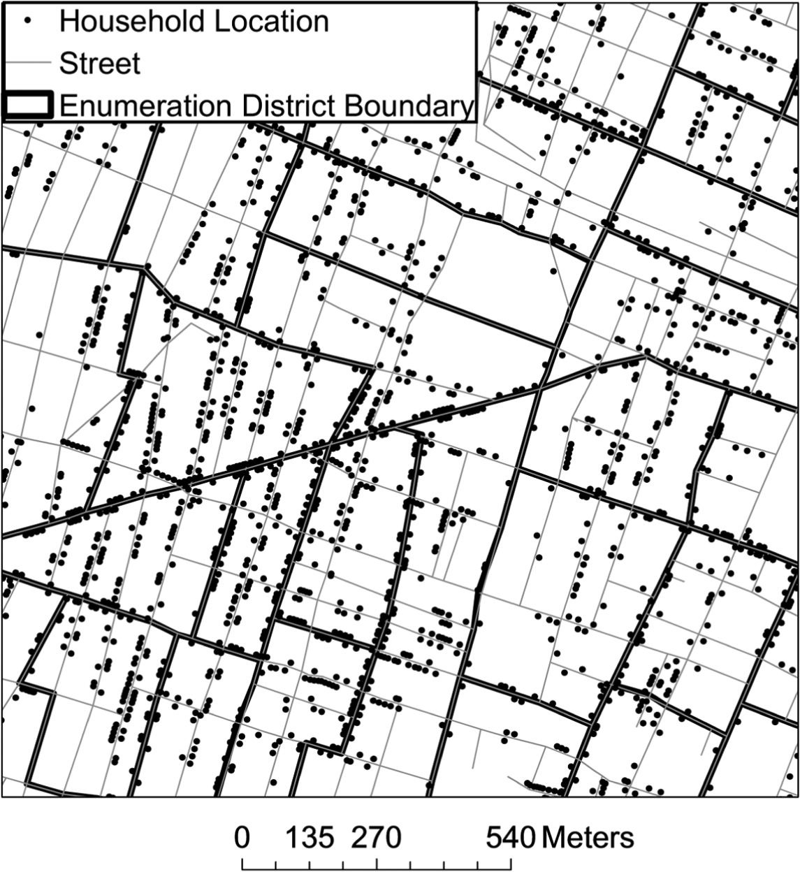
A map showing children’s household locations, streets, and enumeration districts in a part of 1880 Newark, New Jersey.
A total number of 501 death records by June 1885 were identified among 6,762 individuals who were infants (of age 0 to 1 year old) in 1880 Newark. This analysis is focused on the 438 death records among 5,767 infants who were Irish, Germans, or Yankees. These 5,767 cases resided in 5,558 households across 844 street blocks that in turn were nested within 71 EDs. That is, on average, each ED consisted of about 12 street blocks, within each of which seven children lived.
Individual-level predictors include child’s gender and ethnicity. A child’s ethnicity is determined by combining several variables, including race, place of birth, and parents’ places of birth. For example, a white person who was born in Ireland (first-generation immigrant) or who was born in any state of the United States but whose parents were born in Ireland (second-generation immigrant) is coded as an Irish immigrant. Household-level predictors include household header’s age and socioeconomic status, and number of children in the household. Socioeconomic status is measured by a socioeconomic index (SEI) score coded by the Minnesota Population Center based on people’s average education and earnings in each occupation as measured in 1950 and standardized to be a continuous value bounded between 0 and 100 with 0 indicating unemployed.
ED-level predictors include population density, median SEI of household heads, and an ethnic segregation measure known as Simpson’s diversity index. For each ED, a score of Simpson’s diversity index is calculated by assessing ethnic compositions across street blocks that lie within the ED’s boundary as subarea units. A larger score of Simpson’s diversity index reflects more evenly distributed ethnic populations across all street blocks within an ED, whereas a smaller score indicates a tendency for some blocks to be predominated by one ethnic group while other blocks to be occupied by another group. Simpson’s diversity index is normalized to be bounded between 0 (indicating the least ethnic diversity—i.e., a single group dominates the neighborhood) and 1 (indicating greatest ethnic diversity—i.e., all groups appear in the neighborhood with equal proportions).
5.2. Results for Child Mortality Data
Table 4 presents the descriptive statistics of the dependent variable and predictors for child mortality in 1880 Newark, New Jersey. The death rate was highest for Irish children (11%) and lowest for German children (5%). The data were roughly equally stratified by gender. More than half of the children were Yankees, about one-fifth were Irish, and the rest were Germans. The average age of household heads was about 35 years old with little variation by children’s ethnicities. On average, Yankee children lived in the wealthiest households, whereas Irish children lived in the poorest households as measured by the household head’s SEI score. Yankee children also tended to have fewer siblings compared with Irish and German children. As for the neighborhood context, German children lived in the least ethnically diverse yet most crowded EDs compared with Irish and Yankee children. Yankee children lived in slightly wealthier EDs compared with Irish and German children.
Descriptive Statistics of the Child Mortality Data in 1880 Newark, New Jersey

Table 5 presents regression results from the standard multilevel, pure spatial, hybrid CAR, and hybrid spatial logit models where an exponential function for spatial correlation is employed. The DIC values indicate that the hybrid spatial model fits best to the data, followed by the pure spatial, hybrid CAR, and standard multilevel models in descending order. The estimated coefficients of the individual and household-level predictors are roughly the same across the four models. Boys were significantly more likely than girls to die. The risk of death was significantly greater for Irish children, but lower for German children than for Yankee children. Household head’s SEI was negatively associated with child mortality. The main difference in the estimates of fixed-effects arises from the ED-level predictors. Specifically, ED-level ethnic composition as measured by Simpson’s diversity index was estimated to be significantly related to child mortality in the standard multilevel model but not so in the three spatial models. This discrepancy may be attributable to ignoring potential correlations between children living in nearby EDs and hence downward-biased estimates of standard errors in the standard multilevel model, resulting in inflated statistical significance. This is partially supported by visually comparing the posterior estimates from the multilevel and the hybrid models plotted on a map (see Figure 7 and the discussion below). It is also worth noting that the point estimate Simpson’s diversity index is much larger from the standard multilevel model than that from the other models. Therefore, it is unclear whether the other models actually produced biased estimates for this parameter as compared with the standard multilevel model. This discrepancy is worth further investigation in future substantive research.
Estimates of Logit Models of Child Mortality in 1880 Newark, New Jersey
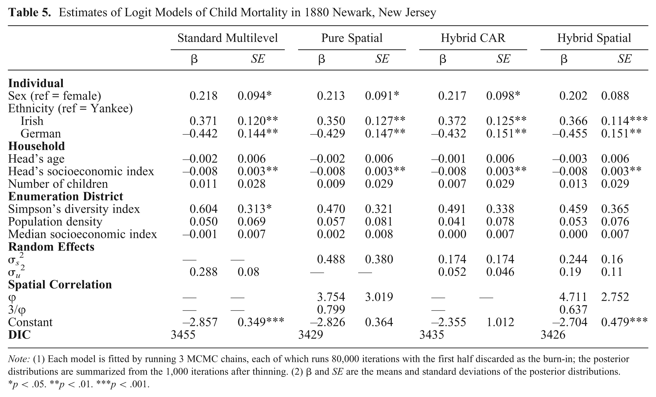
Note: (1) Each model is fitted by running 3 MCMC chains, each of which runs 80,000 iterations with the first half discarded as the burn-in; the posterior distributions are summarized from the 1,000 iterations after thinning. (2) β and SE are the means and standard deviations of the posterior distributions.
*p < .05. **p < .01. ***p < .001.
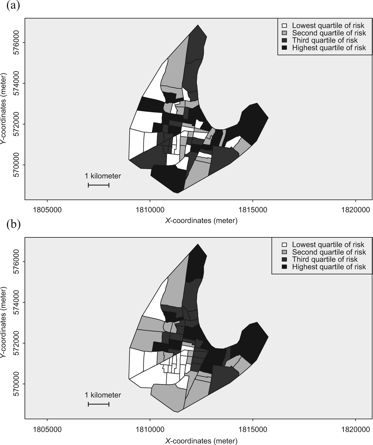
Posterior means of neighborhood effects from the standard multilevel model (a) and that of spatial effects from the hybrid spatial model (b) fitted to the child mortality data of 1880 Newark, New Jersey.
Turning to other parameters, the estimate of
Moreover, the estimate of

Estimates of spatial correlation from distance-based (exponential) pure and hybrid spatial logit models fitted to the child mortality data of 1880 Newark, New Jersey.
6. Discussion
The standard multilevel regressions that are widely used in neighborhood research typically ignore potential between-neighborhood correlation due to underlying spatial processes, and hence they are subject to biased statistical inference. In contrast, spatial models make estimations and predictions over space by explicitly modeling the spatial correlations among observations in different locations. Through systematic comparisons of model estimations and predictions for binary outcomes using both simulation and empirical data, this study sheds new light on the relative strengths and weaknesses of spatial models as compared with the standard multilevel model, and it is informative for future research on neighborhood and spatial effects. The spatial models are particularly applicable to studies of neighborhood effects that involve social and demographic processes across neighborhood boundaries within an urban system.
A few examples in the literature include the spatial dynamics embedded in the effects of neighborhood-level collective efficacy on social control of children (Sampson et al. 1999), violent crimes (Sampson, Raudenbush, and Earls 1997), and birth weight (Morenoff 2003) in Chicago; the impact of neighborhood socioeconomic inequality on children’s achievement in Los Angeles (Sastry and Pebley 2010); and the relation between level of areal flooding and return migration to New Orleans after Hurricane Katrina (Fussell, Sastry, and VanLandingham 2010).
Several important findings stand out from the simulation analysis conducted in this study. First, the standard multilevel and spatial models have similar performance with respect to estimating parameters of fixed effects as well as predicting new observations within existing neighborhoods. In other words, adjusting for either within- or between-neighborhood correlation alone is almost as good as adjusting for both when the main interest is to obtain good estimates of fixed effects predictors or to make partially-out-of sample predictions.
Second, adjusting for only one type of correlation does lead to biased and inaccurate estimates of the variances of random effects, be it in within-neighborhood or between-neighborhood correlations. This may have serious implications for research on neighborhood effects given the common practice of assessing neighborhood effects solely based on the parameter estimate of
Third, there is some evidence of minor advantage of spatially modeling between-neighborhood correlations when it comes to making predictions for observations from an unobserved neighborhood. In such a case, a spatial model has the capacity to borrow strength from observations in nearby neighborhoods and hence is able to improve predictive accuracy, compared with a standard multilevel model that does not pool data across neighborhoods. This advantage is quite limited (only about 2% to 3% higher predictive match rates) and decreases as the strength of spatial correlation decreases relative to that of within-neighborhood correlation. However, this potential merit of spatial modeling has begun to attract researchers who integrate spatial information into social-demographic survey data in order to avoid drawing biased statistical inferences based on the assumption of independence between spatial units (Borgoni and Billari 2003). Nonetheless, hybrid spatial models, be they lattice- or distance-based, are likely to sacrifice their predictive power to better fitting the observed sample data, whereas the pure spatial model sustains its relatively superior performance of fully out-of-sample prediction, despite model misspecifications.
Drawing on geocoded child mortality data of 1880 Newark, this research illustrates the advantages of applying a spatial modeling strategy in empirical demographic research. By taking into account both within- and between-neighborhood correlations, hybrid models are effective at appropriately adjusting for uncertainty in regression estimation and thus avoiding artificially inflated statistical significance. Moreover, the hybrid spatial models allow spatial random effects to be disentangled from nonspatial neighborhood random effects, facilitating the detection of distinct spatial patterns within the population of interest. Nevertheless, distance-based hybrid model can provide extra information about the geographic scale of spatial correlation, which is not readily available in a lattice-based hybrid model.
To conclude, this study demonstrates several merits of spatial modeling that call for researchers to reflect upon the assumption of between-neighborhood independence and the role of space in understanding contextual effects. The application of spatial modeling in neighborhood research may have traditionally been hindered by a lack of appropriate data with enough spatial information. As GIS techniques continue to advance and become more cost-effective, however, social science researchers have now made tremendous progress in incorporating spatial components into large-scale population survey data collection in both developed (e.g., Harris et al. 2009) and developing countries (e.g., Popkin et al. 2010). Future research should take advantage of fast-growing spatial data collection and get equipped with spatial modeling as a common analytical strategy.
Spatial models are not free from limitations, however. First, computational costs remain high despite considerable improvement in computer hardware and the development of new algorithms. For example, model convergence is problematic if a complex distance-decay spatial correlation function such as the Gaussian is adopted. Likewise, exploratory simulation analysis (not shown) suggests that a hybrid spatial model for ordinal or count variables other than binary data very often runs into numerical problems and hence leads to either unstable estimates or failure to converge. Although maximum likelihood estimates or their variants (e.g., pseudo maximum likelihood) other than Bayesian estimates have been developed, they are subject to difficulty in numerical integration for high-dimensional complex data as well. Nevertheless, computational costs for spatial models are likely to be considerably reduced with improvements in algorithms and computer hardware in the near future.
Second, an understated issue in the present study and yet an important one in empirical studies is how neighborhoods or areas are defined. Neighborhood effects involve a process in which place-based membership induces a shared exposure to certain factors either imposed exogenously such as public policy or arising endogenously such as neighborhood collective efficacy. The question then becomes, what place effects are to be modeled (Arcaya et al. 2012) and therefore where should the boundary of the place be drawn? These questions cannot be answered without careful theoretical reasoning and comprehensive knowledge about the substantive subject under study, although certain analytical tools can offer some assistance (Logan et al. 2011). Nevertheless, instead of precluding a spatial modeling approach, these limitations imply considerable opportunities for fruitful future research.
Footnotes
Acknowledgements
The author thanks John R. Logan and the staff of the research initiative on Spatial Structures in the Social Sciences at Brown University for providing the historical GIS data used in this study. The author also acknowledges the support of the computational resources and services provided by the Center for Computation and Visualization, Brown University. The paper benefited greatly from the comments provided by Marcia C. Castro and participants at the 2012 annual meeting of the Population Association of America, and three anonymous reviewers.
Funding
The author disclosed receipt of the following financial support for the research, authorship, and/or publication of this article: Financial support for the research, authorship, and/or publication of this article was provided by the National Science Foundation (grant number 0647584) and the National Institutes of Health (grant number 1R01HD049493–01A2).