Accuracy and variability in early spontaneous word production: The effects of age,frequency and neighbourhood density

Abstract

High rates of error and variability in early word production may signal speech sound disorder. However, there is little consensus regarding the degree of error and variability that may be expected in the typical range. Relatedly, while variables including child age, word frequency and word phonological neighbourhood density are associated with variance in word production accuracy and variability, such effects remain under-examined in spontaneous speech. This study measured the accuracy and variability of 234,551 spontaneous word productions from five typically developing children in the Providence corpus (0;11–4;0). Using Bayesian regression, accuracy and variability rates were predicted by age, input frequency, phonological neighbourhood density, and interactions between these variables. Between 61% and 72% of word productions were both inaccurate and variable according to strict criteria. However loosening these criteria to accommodate production inconsistencies unlikely to be considered erroneous (e.g. the target /æləɡeɪtəɹ/ pronounced /ælɪɡeɪtəɹ/) reduced this figure to between 10% and 17%, with the majority of word productions then classed as accurate and stable (48%–58%). In addition, accuracy was higher and variability was lower in later months of sampling, and for high frequency words and high density words. The author discusses the implications of these results for future research and the differential diagnosis of speech sound disorder, and presents an explanatory account of findings emphasizing the development of oral-motor skills and increasingly detailed phonological word representations.

Keywords

Accuracy corpus analysis phonological neighbourhood density variability word frequency word learning

Introduction

Word learning is often construed as a binary phenomenon: either a child is able to understand or produce a word or not. This is reflected, for instance, in studies using Communicative Development Inventory (CDI) data, in which variables such as word frequency and neighbourhood density may be modelled as predictors of caregiver estimates of age of acquisition (e.g. Braginsky et al., 2019; Jones & Brandt, 2019; Storkel, 2004). It is clear, however, that early word learning is far from black-and-white. Children’s early word productions – the focus of the current study – are often recognizable though inaccurate, and different productions of the same word can vary considerably. For instance, in a landmark study, Ferguson and Farwell (1975) describe a child aged 1;3 (one year; three months) producing 10 variants of the word pen in a 30-minute elicitation. Such observations serve as a reminder that word learning is a dynamic process, in which oral-motor, lexical and phonological development closely interact, and in which word productions typically become more accurate and less variable over time (Macrae, 2013).

The purpose of this study is to examine word accuracy and variability in spontaneous speech from five children recorded between 11 months and four years of age. The novelty of the current analysis is that it provides a more representative account of early word production accuracy and variability than previous work, which has been limited to a small number of target words, utterances, or consonant clusters. In the experimental literature, for instance, Sosa (2015) assessed the production of 25 words; Sosa and Stoel-Gammon (2012) assessed 30 words; Macrae (2013) assessed 20 words; and Betz and Stoel-Gammon (2005) assessed just five words all elicited repeatedly in controlled fashion. Meanwhile, with respect to prior naturalistic analyses, McLeod and Hewett (2008) assessed spontaneous speech samples collected over a six-month period but limited their analysis to words with initial or final consonant clusters that occurred in a subset of 100 utterances. Similarly, Ota and Green (2013) analysed accuracy and variability rates among three children recorded in the Providence corpus (Demuth & McCullough, 2009) – the corpus used in the current study – but limited their analysis to six classes of consonant cluster. In contrast, this study involves the analysis of 234,551 word tokens (4360 types) spoken over a three-year period.

The selection of a small number of target words, utterances, or consonant clusters may be seen as an advantage rather than as a limitation. Restricting the test inventory to a handful of items makes experimentation and analysis more practical and establishes a procedural framework that may be applied in clinical settings, where rates of accuracy and variability are of diagnostic interest and in which time or the child’s attention may be limited. For this reason, measures such as the Word Inconsistency Assessment (developed to identify inconsistent speech disorder; Dodd et al., 2002) test the accuracy and variability of just 25 words. However, it is also likely that an analysis unrestricted by phoneme cluster, word class, syllable, word, or by utterance count, can provide additional insight into early word production accuracy and variability rates, which may in turn improve understanding of early language, memory and oral-motor development. This is the broad aim of the current study.

This article presents two analyses. The first is a descriptive summary of word production accuracy and variability rates for each child in the Providence corpus (Demuth & McCullough, 2009). Following Grunwell (1992), prior experimental studies have categorized word productions into four classes: (i) accurate and stable (i.e. correct across multiple productions); (ii) accurate but variable (i.e. different across productions but including correct forms); (iii) inaccurate but stable; and (iv) inaccurate and variable (e.g. Holm et al., 2007; McLeod & Hewett, 2008; Sosa, 2015). The current study is novel in applying this taxonomy to early spontaneous speech. In the prior literature using this approach there has been special interest in the rate of words produced variably in the absence of accurate forms; this class is termed variable without hits (e.g. Grunwell, 1992, class (iv) listed above; Holm et al., 2007). This is because high rates of variability without hits has been proposed as a marker of early speech sound disorder, which is an umbrella term describing a general difficulty acquiring accurate and intelligible speech in line with peers (Sosa, 2015, p. 24). The production of an excessive number of words categorized as variable without hits has been termed inconsistent speech disorder in order to differentiate this profile from the spoken word error and variability expected within the normal range (e.g. Holm et al., 2007).

A problem with using spoken word inconsistency rates to identify speech sound disorder, however, is that substantial discrepancies in accuracy and variability estimates from studies involving typically developing children make it difficult to determine what constitutes the normal range. For instance, Holm et al. (2007) report on an elicitation task involving 409 typically developing children in which only 13% of words were produced variably at age 3;0–3;5, with this figure dropping to 2.5% by age six. Notably, these authors report that the majority of variable forms produced were variable with hits, and conclude that ‘inconsistency [i.e. variability without hits] is not a feature of normal development at any age’ (Holm et al., 2007, p. 483). In contrast, a number of studies have reported much higher rates of error and variability in typically developing children. McLeod and Hewett (2008), for instance, report a variability rate of 53.7% among children aged 2;0–3;4; Macrae (2013) reports a variability rate of 77.7% among children aged 1;9–3;1; and, in a direct replication of Holm et al. (2007), Sosa (2015) reports a variability rate of 77% among children aged 2;6–2;11, and 57% among children aged 3;6–3;11. Importantly, the most frequent response type reported by Sosa (2015) was variable without hits, which comprised 45% of all responses across age groups for 25 words (range = 4%–76%). Sosa (2015) attributes the discrepancy in estimates with the original Holm et al. (2007) study in part to heightened transcription validity. Sosa (2015) made offline transcriptions of recordings and adopted a so-called consensus procedure in which two or more listeners transcribed each spoken word. In contrast, Holm et al. (2007) used online transcription (i.e. transcriptions were made as the child was speaking) and no consensus procedure, with reliability checks for up to only 10% of the data. Sosa (2015) notes, however, that transcription validity alone cannot fully account for the discrepancy observed. Re-coding the replication study data and ignoring vowel quality differences – which it is argued may be vulnerable to online transcription error – Sosa (2015) reports an overall variability rate of 56%. Although lower than the rate of 68% variability from the initial coding, this revised figure remains considerably higher than the 12% reported by Holm et al. (2007). Ultimately, it is concluded that the reason for the discrepancy in estimates remains difficult to establish, and this may mean that transcription-based assessment is too unreliable for use in a clinical setting. Sosa (2015) argues that the prevalence of variable without hits responses in the typically developing population (observed under both methods of transcription) calls into question the validity of using production inconsistency as a marker for the differential diagnosis of early speech sound disorder. An aim of the current study – specifically the first analysis – is to contribute to ongoing debate regarding the degree of accuracy and variability that may be expected in the normal range.

The second analysis of the current study looks at factors explaining early accuracy and variability rates. Despite between-study discrepancies in estimates, there is general agreement that older children show higher word production accuracy and lower word production variability than younger children (Holm et al., 2007; Macrae, 2013; Sosa, 2015). For this reason, age at word production is included as a predictor in the statistical model of accuracy and variability rates later presented. It is important to note, however, that age is serving here as a proxy variable in lieu of more fine-grained measurements, and that two dominant overlapping mechanisms have been suggested to explain this developmental trend. In one account, early production inaccuracy and variability is attributed to immature oral-motor control (e.g. Kent, 1992). This position is apparently supported by evidence of heightened spatial and temporal variation in the movement of articulators (i.e. jaw, tongue, lips) during childhood (Goffman & Smith, 1999). One limitation of this account, noted by Sosa (2015, p. 33), is that the mapping between motor control and segment production accuracy and variability is imperfect. Goffman et al. (2007), for instance, note that word production can be accurate despite spatial and temporal variation in motor control, while conversely segment production inaccuracy and variability may occur despite apparently mature motor control. There is, nevertheless, good evidence that children’s oral-motor skills develop substantially during the early years, and furthermore that this development correlates with language skills independently of general cognitive ability (e.g. Alcock, 2006). Thus while production error or instability may not always indicate immature or disordered motor control, it would appear reasonable to assume that oral-motor development to some degree underpins children’s developing word production accuracy and stability.

A second and compatible account attributes early word production error and variability to underspecified phonological word representations. In learning a new word, the child must remember that word’s phonological features alongside semantic and pragmatic information. A large number of studies have argued that phonological word representation follows a trajectory from holistic to segmental (Ferguson & Farwell, 1975; Metsala & Walley, 1998; Ventura et al., 2007; Walley, 1993). For instance, older and linguistically advanced children often identify mispronunciations in known words more rapidly and accurately than younger or less advanced peers (e.g. Ainsworth et al., 2016; see also Edwards et al., 2004; Munson et al., 2005, for related evidence with respect to non-word repetition accuracy). This work remains somewhat controversial, with apparently conflicting studies reporting early sensitivity to sub-lexical phonemic detail and mispronunciations (e.g. Swingley & Aslin, 2002). Nevertheless, a broad view is that phonological word representations become increasingly detailed as the lexicon grows, and subsequently with the onset of literacy. One possibility, then, is that holistic phonological word representations provide an insufficient basis for accurate and stable motor planning and output, which evidences in production error and variability in early typical development and protracted speech inconsistency in atypical development (Holm et al., 2007; Sosa, 2015). In line with this position, Macrae and Sosa (2015) report no effect of child age on word production variability when controlling for expressive vocabulary size.

In addition to these child-based factors – i.e. oral-motor and memory/representational development – it is important to acknowledge lexical influences on early word production accuracy and variability. Young children produce certain words more or less accurately or stably than other words (Sosa & Stoel-Gammon, 2006), suggesting that child-based factors interact with specific features of the target word. In order to understand this observation, a number of studies have modelled accuracy and variability rates as a function of lexical variables of specific interest, such as phonological complexity (Macrae, 2013). In the same way, the current study examines how child-directed speech frequency and phonological neighbourhood density affect spoken word accuracy and variability. Frequency effects occur at all levels of linguistic representation (e.g. phoneme, word and syntax), and it is therefore argued that such effects must be accommodated under any credible account of first language acquisition (Ambridge et al., 2015). Prior work using a range of paradigms (e.g. elicitation, naming) shows a negative association between word frequency and error and variability rates (e.g. Sosa & Stoel-Gammon, 2012). This pattern has been attributed to repeated exposure to a target word strengthening the corresponding phonological word representation and therefore providing a fine-grained motor plan.

High phonological neighbourhood density – i.e. phonological similarity between a target word and other words in a given lexicon – is also associated with higher accuracy and more stable word production (e.g. Sosa & Stoel-Gammon, 2012), as well as with lower age of acquisition and better target retention in experimental paradigms (Storkel, 2009; Storkel & Lee, 2011). Such effects are separable from those of word frequency, despite a high correlation between these variables (i.e. high frequency words are usually high density; Storkel, 2004). A dominant explanatory account of this effect is that high neighbourhood density words contain regular sound patterns that are held in short-term memory more precisely during initial processing (e.g. the at in mat, cat and catch; Gathercole et al., 1999). This supports the subsequent formation of detailed phonological word representations in long-term memory, which may in turn provide fine-grained motor plans (Hoover et al., 2010; Metsala & Walley, 1998).

Word frequency and phonological neighbourhood density are also reported to interact in early word learning. For instance, Hollich et al. (2002) and Storkel (2004) report that high neighbourhood density predicted successful acquisition and production for low though not high frequency words. This suggests that high neighbourhood density is important when word frequency is low but that high frequency nullifies the high neighbourhood density advantage. Both neighbourhood density and frequency are also considered to interact with age (Braginsky et al., 2019; Jones & Brandt, 2019). For instance, in a study of 300 British English-speaking children, Jones and Brandt (2019) found that high neighbourhood density and high frequency were more strongly associated with caregiver reports of word production at 12 months than at 25 months. Whether or not similar interactions are associated with degrees of early spontaneous word production accuracy and variability remains unknown.

The current study

This study estimates spontaneous word production accuracy and variability rates in longitudinal data from five American English-speaking children. I present a classification of spontaneous word productions in terms of: (i) accurate and stable; (ii) accurate but variable; (iii) inaccurate but stable; and (iv) inaccurate and variable. The purpose of this analysis is to contribute to ongoing discussion regarding the rates of accuracy and variability that can be expected in the normal range. Given widespread disagreement in the prior literature in this area (e.g. Holm et al., 2007; Sosa, 2015), I made no predictions regarding the results of this analysis. I also present an analysis of accuracy and variability rates modelled as a function of child age, input frequency and ambient language phonological neighbourhood density, both as main effects and in interaction. Based on the literature reviewed, my predictions were that word production accuracy would increase with age, while production variability would decrease with age. I predicted that high frequency and high neighbourhood density would be associated with greater production accuracy and stability, and that these associations would be stronger in earlier periods of sampling. Finally, high neighbourhood density was expected to be more strongly associated with accurate and stable production for low frequency words.

Method

Corpus

This study examined accuracy and variability rates in spontaneous speech recorded in the Providence corpus (Demuth & McCullough, 2009). The Providence corpus contains transcripts of 364 hours of audio and video recordings from six monolingual children (three girls, three boys) aged 0;11–4;0. Data from one child, Ethan, were excluded from the current analysis given this child’s diagnosis of Asperger’s Syndrome at age five. From the onset of first words, children were recorded for a minimum of one hour every two weeks during interaction with their caregivers, ordinarily their mothers. Details of each child’s data are shown in Table 1.

Table 1.

Corpus summary. Showing total recorded utterances and glosses, mean length of utterance (MLU) in morphemes and usable token and type counts. Glosses identifies transcribed strings, whether or not these are words, e.g. ‘mum’, ‘cat’, ‘hmm’, ‘haha’, ‘achoo’. Usable tokens and types identify lexical items (e.g. ‘mum’, ‘cat’) for which independent variable data was available; see Independent variables: age, frequency and neighbourhood density.

Speaker	Age (months)	Utterances	Glosses	MLU	Usable tokens	Usable types
Alex	16–41	29,251	63,727	2.31	31,150	1434
Lily	13–48	40,027	105,003	3.07	58,088	2011
Naima	11–46	43,499	145,783	4.03	72,280	2765
Violet	14–47	17,296	41,924	2.92	20,750	1533
William	16–40	21,291	46,508	2.38	26,361	1314

Transcript format was the major motivation for using the Providence corpus. Recordings are narrowly transcribed in the International Phonetic Alphabet (IPA), and produced word forms are listed alongside target forms. This makes it straightforward to calculate production accuracy and variability scores. A second motivation for using the Providence corpus was that transcription reliability for the corpus is high. After initial transcription, a second trained coder transcribed a sample of 10% of each recording, with inter-rater reliability reported between 80% and 98%. Given its high suitability to early word accuracy and variability research, it is perhaps unsurprising that the Providence corpus has been used in related previous work. Notably, Ota and Green (2013) analysed the effect of input frequency on the production of consonant clusters by three children in this corpus.

Data preparation

Providence corpus data files in Phon software format (Hedlund & Rose, 2019) were accessed via the project website (https://phonbank.talkbank.org/access/Eng-NA/Providence.html) and converted to .csv files in Phon to enable further pre-processing and modelling in R (R Core Team, 2016). Raw .csv files are hosted on the associated project repository alongside an R script allowing readers to re-create all analyses reported in the current study (https://osf.io/w9y27/). These files contain the following columns for each word token: (i) participant name; (ii) participant age; (iii) orthographic word; (iv) IPA target word; and (v) IPA produced form. Analysis in R began with the removal of non-lexical items including conversational sounds such as ‘hmm’, ‘haha’ and ‘achoo’.

Independent variables: age, frequency and neighbourhood density

Independent variable preparation then proceeded with the transformation of participant age into an appropriate format for statistical modelling, e.g. from ‘P1Y10M24D’ to ‘16’ (months). Using the childesr package in R (Sanchez et al., 2018), frequencies for each word produced by each child were then calculated from all American English caregiver transcripts in the CHILDES database (MacWhinney, 2000) in which the children addressed were aged between 22 and 36 months. This included 2,194,651 word tokens and 21,981 word types. Raw counts from this corpus were then log-plus-one transformed. Finally, I retrieved phonological neighbourhood density values for each produced word. In many developmental studies, phonological neighbourhood density is operationalized as the number of words in a given corpus that can be formed by the addition, substitution, or elimination of a single phoneme in a target word, e.g. cat neighbours hat, cot, can and catch (e.g. Stokes, 2014; Storkel, 2004 following Luce & Pisoni, 1998). A general limitation of this operational definition, however, is that it may result in a substantial proportion of words in the corpus being categorized as lexical hermits with zero neighbourhood density (Suárez et al., 2011). Accordingly, the current study adopted a metric of word-level phonological similarity called phonological Levenshtein distance, or PLD20, defined as the mean number of additions, substitutions, or eliminations of phonemes required to change a particular word into its nearest 20 phonological neighbours (Suárez et al., 2011, p. 606). PLD20 values for each word produced were calculated across words in the English Lexicon Project, which provides lexical characteristic data for 40,481 words and which may be considered representative of the ambient language (Balota et al., 2007; retrieved from: www.talyarkoni.com/downloads/pld20.txt). The PLD20 metric is operationalized continuously in order to maximize statistical power. In contrast, the common approach of splitting tokens into high and low density groups has the effect of reducing statistical power, and therefore limiting the quality of inferences that can be drawn. In contrast to plus/minus-one-phoneme metrics of word-level phonological similarity (e.g. Luce & Pisoni, 1998), where a high value equals greater neighbourhood density, a high PLD20 indicates greater phonological distance between a target and its nearest neighbours, or low neighbourhood density. Different criteria of word-level phonological similarity such as the plus-minus-one phoneme criterion and PLD20 are highly correlated, and have been shown to confer analogous effects (Suárez et al., 2011). I therefore strongly expect the results reported below to hold across alternative measures of neighbourhood density.

Predictor correlation and multicollinearity

One limitation of the use of observational data without restriction to a particular target cluster, word, or utterance count is that it is difficult to mitigate the detrimental impact of high predictor correlation. High predictor correlation is an issue because it may cause multicollinearity, which manifests as a distortion of regression model results such as a substantial increase in the size of the estimate or the estimate error, or a shift in estimate direction (e.g. from a positive to a negative value). For this reason, researchers are commonly required to select only variables of personal theoretical interest for testing a specific hypothesis and to omit highly correlated variables that may be of general theoretical interest. In the current study, for instance, high rates of correlation motivated the omission of a word-length variable and alternative word-sound variables including phonotactic probability (note that Storkel, 2004, among others takes the same approach; though see Storkel & Lee, 2011). Correlations between the three predictors included in this study are shown in Table 2.

Table 2.

Pearson correlation matrix for independent variables.

	Age	Frequency	PLD20
Age	1	0.12	−0.05
Frequency	0.12	1	−0.33
PLD20	−0.05	−0.33	1

Notably, a moderate correlation was observed between PLD20 and word frequency (r = −0.33), with high frequency words commonly being high density (i.e. low PLD20). Multicollinearity risk was therefore tested by computing variance inflation factors (VIFs) using the lme4 and car packages in R (Bates et al., 2015; Fox & Weisberg, 2011). These estimates suggested multicollinearity risk was low across predictors, with a maximum value of VIF = 2.61 for the frequency and neighbourhood density interaction term. Recommended maximum VIFs range from 4 to 10 in the literature (e.g. Hair et al., 1995; Pan & Jackson, 2008). In a second assessment of multicollinearity risk I conducted a sensitivity analysis. This involved removing each predictor and re-fitting the main regression model (introduced fully below) to test for changes in the resulting coefficients. No substantial difference in estimates was found during this analysis, in terms of the direction or magnitude of estimates or the size of the estimate errors.

Dependent variables: accuracy and variability

The dependent variables were word production accuracy and word production variability. Numerous operational definitions of each of these variables have previously been used (see Ingram, 2002, for a review). In the current study, the Levenshtein distance between target and actual transcriptions was used as a measure of word accuracy. A word production identical to the listed adult form scored zero and lower accuracy was coded in terms of the number of phonetic insertions, substitutions, or deletions required to turn the produced form into the listed adult form. For instance, if the target word ‘alligator’ listed /æləɡeɪtəɹ/ was produced /ælɪɡeɪɾə/, this production was scored a Levenshtein distance of 3: one change from /ɪ/ to /ə/; one change from /ɾ/ to /t/; and the addition of /ɹ/. Levenshtein distance provides an accuracy metric that is not only intuitive but also computationally efficient. The measure also provides a graded picture of target and produced form distance, in contrast to the binary scoring of accurate and inaccurate forms using zeros and ones sometimes used (e.g. Macrae, 2013).

The second dependent variable of interest was word production variability. For this measure, I followed Ingram (2002, see p. 719 for examples) and used the proportion of whole-word variability (PWV) defined as the number of distinct productions of a word divided by the total number of productions. Where only one distinct form was produced, this form was attributed a variability score of zero. Using tidyverse package functions in R (Wickham et al., 2019), the data were grouped by child and age in months before calculating the degree of variability for each word, produced by each child, within each month of sampling.

The master dataset lists 234,551 word tokens (4360 types) with columns for: (i) speaker name; (ii) speaker age at word production; (iii) orthographic form of word produced; (iv) child-directed speech frequency; (v) phonological neighbourhood density, PLD20; (vi) IPA target form; (vii) IPA produced form; (viii) accuracy (Levenshtein distance); and (ix) variability (PWV) for the produced word in that month of age. This file is available from the project repository (https://osf.io/w9y27/).

Accuracy and variability profiles

One aim of this study was to adopt Grunwell’s (1992) conventions to provide accuracy and variability profiles based on spontaneous speech from five children, without restriction to a particular lexical subset. To do this, conditional statements were used in R to divide all tokens from the master dataset into four classes, before calculating the proportion of produced words within each class for each child. For each of the 234,551 tokens produced, classification worked as follows:

If target / actual distance = 0 and variability = 0, then class = ‘Hit / stable’.

If target / actual distance = 0 and variability > 0, then class = ‘Hit / variable’.

If target / actual distance > 0 and variability = 0, then class = ‘Miss / stable’.

If target / actual distance > 0 and variability > 0, then class = ‘Miss / variable’.

As discussed in the introduction, there has been specific interest in the rate of words produced variably without hits in the typically developing population (i.e. statement 4 above; ‘Miss / variable’). Estimating this rate in spontaneous speech from typically developing children may improve our understanding of expected rates of accuracy and variability, and in turn help determine whether a high rate of variability without hits constitutes a useful clinical marker. Note that in this analysis accuracy is calculated for each word production, while variability is calculated across all productions of each word during each month.

During peer review two anonymous reviewers raised concerns that the coding method presented above may be too stringent. It was noted, for instance, that the production of /æləɡeɪtəɹ/ as /ælɪɡeɪɾə/ may be considered accurate as the vowel change from /ə/ to /ɪ/, the use of /ɾ/ instead of /t/, and the dropping of the word-final /ɹ/ do not constitute errors per se and may be attributable to dialectical variation. Along similar lines, it was suggested that requiring zero variability might be an unrealistic standard given that tokens are being collapsed across a month of sampling. These points are well taken, and in line with the reviewer suggestions I present a second accuracy and variability taxonomy with the modified standards listed below. Note that <= indicates ‘smaller than or equal to’, while >= indicates ‘greater than or equal to’.

If target / actual distance <= 1 and variability <= 0.1, then class = ‘Hit / stable’.

If target / actual distance <= 1 and variability >= 0.1, then class = ‘Hit / variable’.

If target / actual distance >= 1 and variability <= 0.1, then class = ‘Miss / stable’.

If target / actual distance >= 1 and variability >= 0.1, then class = ‘Miss / variable’.

These modified standards allow for minimal deviation from the listed adult form: a Levenshtein distance of zero or one phoneme, and variability of 10% across productions. I encourage readers to experiment further by modifying these threshold values (i.e. 1, 0.1) in the Boolean statements listed in the R code associated with this article (https://osf.io/w9y27/).

Statistical modelling

The second analysis looks at child and lexical influences on word production accuracy and variability. To do this, the brms package (Bürkner, 2018) was used to fit two simple Bayesian regression models in R. In model 1, accuracy (Levenshtein distance) was predicted by (i) the child’s age at production; (ii) the word’s child-directed speech frequency; and (iii) the word’s phonological neighbourhood density (PLD20) in the ambient language. In model 2, variability (for each target word during each month of age) was predicted by (i) the child’s age at production; (ii) the word’s child-directed speech frequency; and (iii) the word’s neighbourhood density (PLD20) in the ambient language. Given known interactions between these variables (e.g. Storkel, 2004), interaction terms were also included for each combination of predictors, i.e. age:frequency, age:PLD20 and frequency:PLD20. All predictors were centred (i.e. M = 0) prior to model fitting. This explains the presence of zeros and negative values (e.g. negative frequencies) on the x-axes of the figures that follow (see Modelling results). In both models, brms package default priors were used (see R code), which I expected to be overwhelmed by the large number of observations (i.e. 234,551 cases). These models fitted well, with a large number of effective samples, stationary and well-mixing chains, rhats uniformly at 1, and good posterior predictive checks (see R code for detailed diagnostics, and the brms package documentation for a detailed description of diagnostic terminology; Bürkner, 2018).

The goal of modelling is to estimate parameters (e.g. β, the beta coefficient) that define the relationship between variables of interest – in this case the relationship between age, frequency and neighbourhood density (main effects and interactions), and rates of spontaneous word production accuracy and variability. In Bayesian statistics the outcome of modelling is a probability distribution that describes the plausibility of different values of the parameter of interest (e.g. β). One motivation for this approach is that it communicates uncertainty in the data better than an emphasis on point estimates such as p values. Of particular interest in this study is the beta parameter estimate, β; i.e. the slope for the regression line for each predictor and response. A distribution for β bound above zero (e.g. 0.2 to 0.5) suggests a positive association between variables. That is, as the predictor value increases so does the response value; there is an upward-sloping regression line. A distribution for β bound below zero (e.g. −0.5 to −0.2) suggests a negative association between the predictor and outcome, i.e. as the predictor value increases the response value decreases; there is a downward-sloping regression line. And a distribution for β spanning zero (e.g. −0.2 to 0.2) suggests no linear relationship between predictors, i.e. a flat regression line, is plausible.

Results

Accuracy and variability profiles

Table 3 shows accuracy and variability profiles for each child, based on the conventions developed by Grunwell (1992) and shown in the Method, Accuracy and variability profiles section as conditional statements (i.e. under the initial zero distance / zero variability criterion). Percentages of forms within each class do not differ substantially between children, despite differences in the rates of usable forms (see Table 1). Importantly, miss / variable rates were high across children, with inaccurate productions of variable words comprising between 61% and 72% of all productions. Hit / stable, i.e. consistently accurate, was the least common production type, ranging from 4% to 7%.

Table 3.

Proportions of words produced within each accuracy and variability class, under the initial zero distance / zero variability criterion.

Speaker	Hit / stable	Hit / variable	Miss / stable	Miss / variable
Alex	0.04	0.16	0.10	0.71
Lily	0.06	0.18	0.14	0.61
Naima	0.04	0.17	0.09	0.69
Violet	0.07	0.18	0.15	0.61
William	0.04	0.14	0.11	0.72

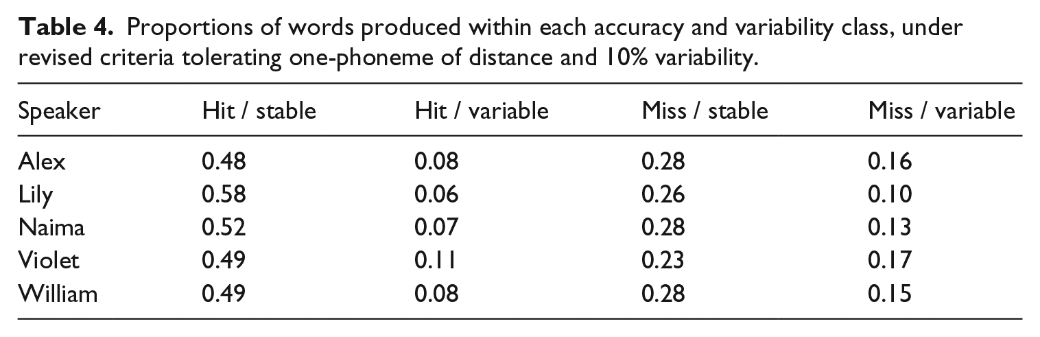
In Table 4, I report the results of the categorization using less strict criteria in which discrepancies of one phoneme and variability of up to 10% were allowed. To re-cap, this approach was prompted by a concern that the criteria generating the results shown in Table 3 were too stringent, and that these criteria would qualify fair deviations from the corpus target listing as errors. Table 4 shows that the proportion of words in each category again ranks similarly across participants. However, there is a substantial difference in the proportions across categories relative to those reported in Table 3. Under the revised criteria, hit / stable is the most common production type, followed by miss / stable, miss / variable and hit / variable. Criteria selection therefore has a substantial impact on the shape of the taxonomy.

Table 4.

Proportions of words produced within each accuracy and variability class, under revised criteria tolerating one-phoneme of distance and 10% variability.

Speaker	Hit / stable	Hit / variable	Miss / stable	Miss / variable
Alex	0.48	0.08	0.28	0.16
Lily	0.58	0.06	0.26	0.10
Naima	0.52	0.07	0.28	0.13
Violet	0.49	0.11	0.23	0.17
William	0.49	0.08	0.28	0.15

Modelling results

Regression model summaries are presented in the Appendix. Figure 1 shows marginal effects from model 1, in which production accuracy (Levenshtein distance) was predicted by child age, child-directed speech frequency and ambient language neighbourhood density (PLD20). Production accuracy improved with age, with a reduction in target / actual distance in later months of sampling (β = −0.03; lower 95% credible interval = −0.03; upper 95% credible interval = −0.03). Words that occurred at relatively high frequency in child-directed speech were produced more accurately than low frequency words (β = −0.12; lower 95% CI = −0.12; upper 95% CI = −0.12). Finally, words with many neighbours in the ambient language were produced more accurately than words with few neighbours in the ambient language (β = 0.10; lower 95% CI = 0.10; upper 95% CI = 0.10).

Figure 1.

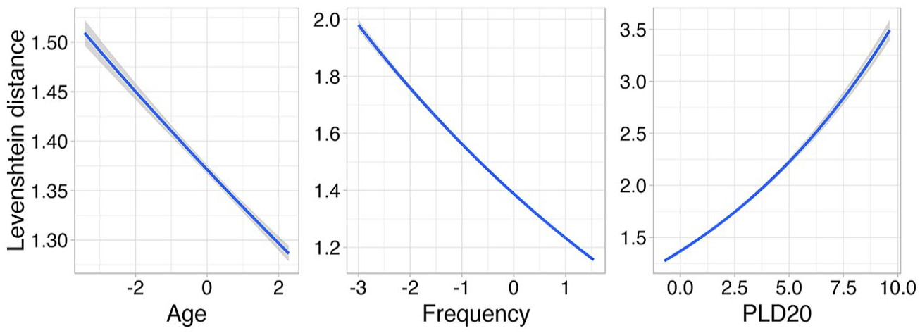
Associations between child age (0;11–4;0), word frequency and phonological neighbourhood density (PLD20), and production accuracy (Levenshtein distance). Shading represents the 95% credible intervals, i.e. the range in which the parameter value falls with 95% probability. Note the scale differences on the y-axes.

I also tested for interactions between age, frequency and PLD20 as predictors of word production accuracy. The results of this analysis are shown in Figure 2. No interaction was found between age and word frequency (β = 0.00; lower 95% CI = 0.00; upper 95% CI = 0.00), indicating that the strength of association between frequency and production accuracy did not change during the sampling period. The interaction between age and PLD20 was marginally negative (β = −0.01; lower 95% CI = −0.01; upper 95% CI = 0.00), indicating that low phonological distance (i.e. high density) is a more important predictor of accurate word production in early rather than late development. Finally, there was a negative interaction between word frequency and PLD20 (β = −0.02; lower 95% CI = −0.03; upper 95% CI = −0.02), indicating that as word frequency increased the association between high density and word production accuracy weakened.

Figure 2.

Interactions between: (i) child age (0;11–4;0) and frequency; (ii) child age and neighbourhood density (PLD20); and (iii) frequency and neighbourhood density (PLD20), with respect to the accuracy response (Levenshtein distance). To ease the interpretation of interactions, age and PLD20 are binned into three levels by default by the brms package (i.e. high, mid, low). Shading represents the 95% credible intervals. Note the scale differences on the y-axes.

Figure 3 shows posterior probability distributions from model 2, in which the proportion of whole-word variability (PWV) was predicted by child age, child-directed speech frequency and neighbourhood density (PLD20). Production variability declined with age, with lower PWV scores in later months of sampling (β = −0.02; lower 95% credible interval = −0.03; upper 95% credible interval = −0.02). Words that occurred at relatively high frequency in child-directed speech were produced more stably than low frequency words (β = −0.48; lower 95% CI = −0.48; upper 95% CI = −0.47). Finally, there was a positive association between PLD20 and word variability (β = 0.10; lower 95% CI = 0.10; upper 95% CI = 0.11), indicating that words that sounded similar to many other words in the ambient language were produced more stably than words that sounded similar to few other words in the ambient language.

Figure 3.

The associations between child age (0;11–4;0), word frequency and phonological neighbourhood density (PLD20), and production variability. Shading represents the 95% credible intervals. Note the scale differences on the y-axes.

I also tested for interactions between age, frequency and PLD20, as predictors of word production variability. The results of this analysis are shown in Figure 4. The interaction between age and frequency was marginally positive (β = 0.02; lower 95% CI = 0.01; upper 95% CI = 0.02), indicating that high frequency words tended to be produced stably across the sampling period, while low frequency words tended to be produced more stably in later months of sampling. The interaction between age and PLD20 was also positive (β = 0.02; lower 95% CI = 0.02; upper 95% CI = 0.03), indicating that in earlier months of sampling word productions were often variable regardless of a word’s neighbourhood density, but that in later months variability was particularly high for low-density words. Finally, there was a positive interaction between word frequency and PLD20 (β = 0.01; lower 95% CI = 0.01; upper 95% CI = 0.02). This suggests that variability for a low frequency word was often high regardless of that word’s PLD20. However, productions of high frequency words were marginally more stable for words that sounded similar to many other words in the ambient language.

Figure 4.

Interactions between: (i) child age (0;11–4;0) and frequency; (ii) child age and neighbourhood density (PLD20); and (iii) frequency and neighbourhood density (PLD20), with respect to the variability response. To ease the interpretation of interactions, age and PLD20 are binned into three levels by default by the brms package (i.e. high, mid, low). Shading represents the 95% credible intervals. Note the scale differences on the y-axes.

Discussion

This study presented two analyses. First, I estimated overall rates of word production accuracy and variability in the spontaneous speech of five typically developing children recorded between the ages of 0;11 and 4;0. The aim here was to contribute to ongoing debate regarding the rates of error and variability that may be expected in the typical range, and relatedly to debate regarding whether a high rate of word production inaccuracy and variability can provide a useful marker of speech sound disorder. Second, the study used Bayesian regression to model word production accuracy and variability as a function of age, frequency, neighbourhood density, and interactions between these variables. While these variables have previously been linked with word production accuracy and variability effects in experimental studies (e.g. Macrae, 2013), such effects remained poorly understood with respect to early spontaneous speech. The results from each analysis are discussed in the following sections.

Accuracy and variability profiles

Following Grunwell (1992) and others (e.g. Holm et al., 2007; McLeod & Hewett, 2008; Sosa, 2015), spontaneously produced words were categorized into four classes: (i) accurate and stable; (ii) accurate but variable; (iii) inaccurate but stable; and (iv) inaccurate and variable. These classes were then populated according to two criteria. Under the first criterion, spoken word productions were classified as accurate and stable only if they did not differ from the listed adult form. This approach broadly replicates the experimental method of Sosa (2015, p. 28). The results of this analysis (Table 3) indicated high rates of error and variability broadly in line with Macrae (2013), McLeod and Hewett (2008) and Sosa (2015), and in contrast to the relatively low estimates presented by Holm et al. (2007). Under this criterion, up to three quarters of the words produced by children in the Providence corpus were variable without hits, which, as in some prior work (e.g. Sosa, 2015), was the most frequent production type. Apparently in direct contrast to Holm et al.’s (2007) claim that ‘inconsistency [i.e. variability without hits] is not a feature of normal development at any age’ (p. 483), the results shown in Table 3 of the current study imply that young typically developing children are highly inconsistent in their early word productions. This in turn makes it reasonable to suggest, following Sosa (2015, p. 33), that overall variability rates – particularly rates of variability without hits – may not provide a useful index to aid the differential diagnosis of children with speech sound disorder.

Under a second criterion, however, spoken word tokens were classified as accurate despite differing from the listed adult target form by a single phoneme, and classified as stable across multiple productions up to a 10% variability threshold. These modifications to the initial criteria were prompted by concerns raised during peer review that the original approach may unfairly qualify reasonable deviations from the adult target listing as errors. This point is well taken, and closely examining the data I found a number of examples supporting the anonymous reviewers’ claims: /mɑm/, for example, pronounced /mʌm/. Though unlikely to be considered erroneous by many listeners, such productions were classed as erroneous under the criteria first used.

As might be expected, the change in criteria had a dramatic impact on the accuracy and variability profiles derived (Table 4). Under the revised criteria, hit / stable was the most common production type (48%–58%), while miss / variable comprised between just 10% and 16% of productions. These figures appear broadly continuous with Holm et al.’s (2007) estimate of 13% variability in 409 typically developing children aged 3;0–3;5 (Holm et al., 2007) as well as with the previously-cited conclusion that production inconsistency is not a feature of typical language development. The revised results (Table 4) suggest that although young children do deviate minimally from the listed adult form used as a standard, they remain generally accurate and stable in their spontaneous word productions, and this in turn constitutes support for the claim that a high overall inaccuracy and variability rate may be considered a valid marker of speech sound disorder (Holm et al., 2007).

Increasing the thresholds used during classification to a Levenshtein distance of 1 and variability of 10% successfully accommodates productions that deviate from the adult listed form but which are unlikely to be considered erroneous. However, this approach comes with a significant cost, as loosening the thresholds permits the classification of minimal errors as accurate forms. This may appear particularly damaging with respect to short words, which dominate the early productive lexicon. The mode length of words in the Providence corpus is three phonemes (M = 3.74), and 155,088 tokens – or 66% of the corpus – comprise three phonemes or fewer. For such words one discrepant phoneme may represent a substantial erroneous deviation, which is ignored under the relaxed thresholds. For example, instances classed as accurate productions under the revised criteria include the production of /bæɡ/ as /bæk/, the production of /bæθ/ as /bæ/, and the production of /bæt/ as /bɛt/. Inspecting the data, such instances appear far from exceptional. Setting a hard and fast decision boundary for the quantification of accurate and variable spoken word forms therefore involves a difficult trade-off: (i) categorize a level of apparently tolerable production deviance as erroneous or (ii) categorize minimal production errors as accurate. When comparing child productions to adult listed forms, this trade-off would apparently exist whether considering large-scale spontaneous speech data such as those of the current study or small-scale elicited speech data, such as those of prior experimental studies (e.g. Holm et al., 2007; Sosa, 2015).

Unfortunately it is impossible to select between the contrasting taxonomies presented in this study on the basis of the current or existing data. Each criteria is well justified, and each generates a taxonomy with proportions of accuracy and variability broadly continuous with those previously reported (e.g. Holm et al., 2007; Sosa, 2015). Given the apparent sensitivity of spoken word classification to minimal changes in the underlying criteria, and given the extensive discrepancies in rates of accuracy and variability reported in the existing literature, it remains unclear whether accuracy and variability profiles can provide a useful method of identifying speech sound disorder. It may well be, as Sosa (2015, p. 32) writes, that:

The use of phonetic transcription to quantify [accuracy and] variability is too unreliable to be used for differential diagnosis of speech sound disorder; more refined acoustic and/or kinematic analysis methods may be needed.

Establishing a robust method of quantifying the degree of spoken word accuracy and variability that occurs in early naturalistic and elicited speech constitutes an important part of the future research agenda, both for our understanding of typical and atypical language development and for the purposes of assessment and intervention. One conceivable direction for future research would be to collect large samples of child, spontaneous and elicited speech data, and then to record accuracy judgements for specific spoken word tokens within those data from a large group of impartial adult listeners. Listeners would hear spoken word instances and identify (for instance via button pressing) whether they considered each token to be accurate or inaccurate (e.g. /æləɡeɪtəɹ/ produced /ælɪɡeɪtəɹ/ and /ælɪɡeɪɾə/). These accuracy judgements could then form a basis for the classification of spoken word tokens into accuracy and variability taxonomies. This study would be highly resource intensive and the method clearly could not be applied directly in clinical contexts. However such an approach may provide the baseline data needed to break the apparent deadlock and help resolve widespread disagreement in the existing literature on early spoken word accuracy and variability rates.

Age and lexical effects on accuracy and variability

The second part of this study looked at child and lexical influences on early rates of spoken word accuracy and variability. The child-related predictor of interest was age, which has previously been reported to have a positive association with word production accuracy and a negative association with word production variability (Holm et al., 2007; Macrae, 2013). The current analysis is the first to confirm that these findings hold in longitudinal spontaneous speech across a sampling age range considerably larger than that of any prior study (i.e. 0;11–4;0). That is, I reported that both error and variability were lower in the later months sampled. The first lexical predictor of interest was child-directed speech frequency, a variable central to the study of early language acquisition which has previously been positively linked to spoken word accuracy and stability (e.g. Sosa & Stoel-Gammon, 2012). The current study also replicated this finding, reporting a robust association between high frequency, and better accuracy and reduced variability. The second lexical predictor of interest was phonological neighbourhood density (PLD20), which has been positively linked to memorization and production advantages (e.g. Storkel, 2004, 2009; Storkel & Lee, 2011). As in Sosa and Stoel-Gammon, (2012), I reported heightened accuracy and reduced variability for high neighbourhood density words, and in doing so demonstrated that previous findings scale-up when assessing children’s spontaneous speech without restriction to a spoken word token limit (e.g. Sosa & Stoel-Gammon, 2012, assessed 30 elicited words).

Modelling also suggested interactions between age, word frequency and phonological neighbourhood density as predictors of spoken word accuracy and variability. For instance, I reported that in early months of sampling productions were highly variable regardless of the words’ neighbourhood density but that in later months of sampling high density (i.e. low PLD20) words were substantially less variable (Figure 4, centre panel). The current study also corroborated previous work by Hollich et al. (2002) and Storkel (2004), who found that high neighbourhood density predicted word acquisition for low but not high frequency words. Such findings contribute to a developing picture of high word exposure frequency as a primary force driving growth of the lexicon, and alternative word characteristics such as high neighbourhood density ‘stepping in’ and supporting learning when exposure frequency is relatively low. The results of this study show for the first time that this effect extends to the accuracy of children’s early spontaneous word productions (Figure 2, right panel).

With the exception of Ethan, who was excluded from the current analyses on the basis of a later diagnosis of Asperger’s Syndrome, children in the Providence corpus are typically developing. It is therefore important to understand the associations between predictors and accuracy and variability rates reported here as part of a typical trajectory, i.e. not within the framework of speech sound disorders. Explanatory accounts compatible with the results reported in this study emphasize oral-motor maturity and a shift from holistic to segmental word representations. There is evidence that children’s oral-motor skills are associated with their language skills independently of their general cognitive abilities (Alcock, 2006). Thus, although further experimentation is required, it may be reasonable to assume that increases in production accuracy and stability with age are to some degree attributable to improved control of the articulators. In addition, early word phonology may be memorized only approximately as a result of working memory limitations or initial focus on relatively holistic word features (Metsala & Walley, 1998), and accurate and stable production will be compromised in the absence of a mental representation detailed enough to provide a solid motor plan. High frequency, high density words hold an advantage in this early trajectory of oral-motor and cognitive development because they are repeatedly encountered and encoded in memory both explicitly and implicitly. High input frequency, high density words are also likely to be produced by the child more regularly, and contain familiar sound patterns that may require minimal articulatory and cognitive recourses. Assessing this emergent explanatory account remains an important ongoing research line, both for its contribution to our general understanding of the interaction between early oral-motor and cognitive development, and for our understanding of how to improve phonological word representation and production in children with developmental language disorder. The current study constitutes an important addition to our understanding of how developmental stage, exposure frequency and phonological neighbourhood density influence the dynamics of early word production accuracy and variability.

Limitations

Despite its contributions to the literature the current study has a number of limitations. I have already discussed the issue of multicollinearity, which prevents against the inclusion of alternative variables of theoretical interest such as phonotactic probability. This is regrettably unavoidable, and I can only encourage readers to use the published code to experiment with different configurations of predictor variables that may be of personal theoretical interest (https://osf.io/w9y27/). A second issue is that at a number of points in this article I draw parallels between the estimates I derived under different criteria of accuracy and variability and the estimates reported in prior studies (e.g. Holm et al., 2007; Sosa, 2015). However, given differences in the sampling methods of the current study and previous work presenting accuracy and variability profiles (e.g. Holm et al., 2007, evaluated variability across only three repetitions), such comparisons are imperfect. It is acknowledged, for instance, that there is more opportunity for word production error and variability in spontaneous speech than there is during elicitation tasks, and that the possibility of spoken word error or variability grows with rates of production, which are not uniform across words in the corpus (McLeod & Hewett, 2008). Furthermore, it is noted that the Providence corpus uses a narrow transcription, while some prior studies (e.g. Sosa, 2015) have made broad transcriptions. Finally, in the introduction to the current study it was argued that the analysis of spontaneous speech data unrestricted by a target cluster, word type, or utterance count can provide insight beyond the analysis of a small number of target words elicited in an experimental setting, for instance by supporting or challenging the validity of such experimental data. I believe the current study to have delivered on this claim not only by raising important questions regarding methods of quantifying early accuracy and variability rates, but also by showing for the first time that a range of findings from the early word acquisition literature (e.g. age, frequency, neighbourhood density effects and interactions) can be found in accuracy and variability rates derived from large-scale, longitudinal, naturalistic word production data. That said, an important trade-off of the use of longitudinal data with a relatively high sampling rate such as the Providence corpus is that because the collection and transcription of such data is both challenging and highly time-consuming participant numbers are often low. A further limitation of the current study is, therefore, that it includes data from just five children, making it difficult to extrapolate findings to the broader population.

Conclusion

This study examined rates of spontaneous word production accuracy and variability with respect to three predictor variables: child age, word frequency and word phonological neighbourhood density. Increases in accuracy and decreases in variability between the ages of 11 months and four years were interpreted within a framework of early memory and oral-motor development – a trajectory within which high exposure frequency and high neighbourhood density confer acquisition and production advantages. I also presented two taxonomies of early accuracy and variability rates that highlighted the difficulty of setting hard and fast error discrimination thresholds. I proposed an accuracy judgement study that may address this issue and help resolve widespread disagreement regarding the rates of accuracy and variability expected within the typical range. Without such normative data it may be difficult to determine the validity of measures of spoken word accuracy and variability used in research and clinical settings.

Footnotes

Appendix

ORCID iD

Samuel David Jones

Supplemental material

An online repository containing all data and code required to reproduce this analysis can be found at:

References

Ainsworth

Welbourne

Hesketh

(2016). Lexical restructuring in preliterate children: Evidence from novel measures of phonological representation. Applied Psycholinguistics, 37(4), 997–1023. https://doi.org/10.1017/S0142716415000338

Alcock

(2006). The development of oral motor control and language. Down Syndrome Research and Practice, 11(1), 1–8. https://doi.org/10.3104/reports.310

Ambridge

Kidd

Rowland

C. F.

Theakston

A. L.

(2015). The ubiquity of frequency effects in first language acquisition. Journal of Child Language, 42(2), 239–273. https://doi.org/10.1017/S030500091400049X

Balota

D. A.

Yap

M. J.

Cortese

M. J.

Hutchison

K. A.

Kessler

Loftis

Neely

J. H.

Nelson

D. L.

Simpson

G. B.

Treiman

(2007). The English Lexicon Project. Behavior Research Methods, 39(3), 445–459. www.ncbi.nlm.nih.gov/pubmed/17958156

Bates

Maechler

Bolker

Walker

(2015). Fitting linear mixed-effects models using lme4. Journal of Statistical Software, 67(1), 1–48. www.jstatsoft.org/v67/i01/

Betz

S. K.

Stoel-Gammon

(2005). Measuring articulatory error consistency in children with developmental apraxia of speech. Clinical Linguistics & Phonetics, 19(1), 53–66. https://doi.org/10.1080/02699200512331325791

Braginsky

Yurovsky

Marchman

V. A.

Frank

M. C.

(2019). Consistency and variability in word learning across languages. Open Mind, 3, 52–67. https://doi.org/10.31234/osf.io/cg6ah

Bürkner

P.-C.

(2018). Bayesian regression models using ‘Stan’. Journal of Statistical Software, 80, 1–28. https://doi.org/10.18637/jss.v080.i01

Demuth

McCullough

(2009). The prosodic (re)organization of children’s early English articles. Journal of Child Language, 36(1), 173–200. https://doi.org/10.1017/S0305000908008921

10.

Dodd

Hua

Crosbie

Holm

Ozanne

(2002). Diagnostic evaluation of articulation and phonology—U.S. Edition (DEAP) [Technical report]. Pearson.

11.

Edwards

Beckman

M. E.

Munson

(2004). The interaction between vocabulary size and phonotactic probability effects on children’s production accuracy and fluency in nonword repetition. Journal of Speech, Language, and Hearing Research, 47(2), 421–436. https://doi.org/10.1044/1092-4388(2004/034)

12.

Ferguson

C. A.

Farwell

C. B.

(1975). Words and sounds in early language acquisition. Language, 51, 419–439. https://doi.org/10.1017/CBO9780511980503.007

13.

Fox

Weisberg

(2011). An {R} companion to applied regression (2nd ed.). SAGE. http://socserv.socsci.mcmaster.ca/jfox/Books/Companion

14.

Gathercole

S. E.

Frankish

C. R.

Pickering

S. J.

Peaker

(1999). Phonotactic influences on short-term memory. Journal of Experimental Psychology: Learning Memory and Cognition, 25(1), 84–95. https://doi.org/10.1037/0278-7393.25.1.84

15.

Goffman

Gerken

Lucchesi

(2007). Relations between segmental and motor variability in prosodically complex nonword sequences. Journal of Speech, Language, and Hearing Research, 50(2), 444–458. https://doi.org/10.1044/1092-4388(2007/031)

16.

Goffman

Smith

(1999). Development and phonetic differentiation of speech movement patterns. Journal of Experimental Psychology: Human Perception and Performance, 25(3), 649–660. https://doi.org/10.1037/0096-1523.25.3.649

17.

Grunwell

(1992). Assessment of child phonology in the clinical context. In Ferguson

C. A.

Menn

Stoel-Gammon

(Eds.), Phonological development: Models, research, implications (pp. 457–483). York Press.

18.

Hair

J. F.

Jr. Anderson

R. E.

Tatham

R. L.

Black

W. C.

(1995). Multivariate data analysis (3rd ed.). Macmillan.

19.

Hedlund

Rose

(2019). Phon 3.0. [Computer software]. www.phon.ca/phon-manual/misc/Welcome.html

20.

Hollich

Jusczyk

P. W.

Luce

P. A.

(2002, January). Lexical neighborhood effects in 17-month-old word learning. In Proceedings of the 26th Annual Boston University Conference on Language Development (pp. 314–323). Cascadilla Press.

21.

Holm

Crosbie

Dodd

(2007). Differentiating normal variability from inconsistency in children’s speech: Normative data. International Journal of Language and Communication Disorders, 42(4), 467–486. https://doi.org/10.1080/13682820600988967

22.

Hoover

J. R.

Storkel

H. L.

Hogan

T. P.

(2010). A cross-sectional comparison of the effects of phonotactic probability and neighborhood density on word learning by preschool children. Journal of Memory and Language, 63(1), 100–116. https://doi.org/10.1016/j.jml.2010.02.003

23.

Ingram

(2002). The measurement of whole-word productions. Journal of Child Language, 29(4), 713–733. https://doi.org/10.1017/S0305000902005275

24.

Jones

S. D.

Brandt

(2019). Do children really acquire dense neighborhoods? Journal of Child Language, 46(6), 1260–1273. https://doi.org/10.1017/S0305000919000473

25.

Kent

R. D.

(1992). The biology of phonological development. In Ferguson

C. A.

Menn

Stoel-Gammon

(Eds.), Phonological development: Models, research, implications (pp. 65–90). York Press.

26.

Luce

P. A.

Pisoni

D. B.

(1998). Recognizing spoken words: The neighborhood activation model. Ear and Hearing, 19(1), 1–36. https://doi.org/10.1097/00003446-199802000-00001

27.

Macrae

(2013). Lexical and child-related factors in word variability and accuracy in infants. Clinical Linguistics & Phonetics, 27(6–7), 497–507. https://doi.org/10.3109/02699206.2012.752867

28.

Macrae

Sosa

A. V.

(2015). Predictors of token-to-token inconsistency in preschool children with typical speech-language development. Clinical Linguistics & Phonetics, 29(12), 922–937. https://doi.org/10.3109/02699206.2015.1063085

29.

MacWhinney

(2000). The CHILDES project: Tools for analyzing talk (3rd ed.). Lawrence Erlbaum. http://talkbank.org/manuals/CLAN.pdf

30.

McLeod

Hewett

S. R.

(2008). Variability in the production of words containing consonant clusters by typical 2- and 3-year-old children. Folia Phoniatrica et Logopaedica, 60(4), 163–172. https://doi.org/10.1159/000127835

31.

Metsala

J. L.

Walley

A. C.

(1998). Spoken vocabulary growth and the segmental restructuring of lexical representations: Precursors to phonemic awareness and early reading ability. In Metsala

J. L.

Ehri

L. C.

(Eds.), Word recognition in beginning literacy (pp. 89–120). Lawrence Erlbaum.

32.

Munson

Edwards

Beckman

M. E.

(2005). Relationships between nonword repetition accuracy and other measures of linguistic development in children with phonological disorders. Journal of Speech, Language, and Hearing Research, 48(1), 61–78. https://doi.org/10.1044/1092-4388(2005/006)

33.

Ota

Green

S. J.

(2013). Input frequency and lexical variability in phonological development: A survival analysis of word-initial cluster production. Journal of Child Language, 40(3), 539–566. https://doi.org/10.1017/S0305000912000074

34.

Pan

Jackson

R. T.

(2008). Ethnic difference in the relationship between acute inflammation and serum ferritin in US adult males. Epidemiology and Infection, 136, 421–431.

35.

R Core Team. (2016) R: A language and environment for statistical computing. R Foundation for Statistical Computing. www.R-project.org/

36.

Sanchez

Meylan

Braginsky

MacDonald

Yurovsky

Frank

(2018). childes-db: A flexible and reproducible interface to the child language data exchange system. Behavior Research Methods, 51(4), 1928–1194. https://psyarxiv.com/93mwx

37.

Sosa

A. V.

(2015). Intraword variability in typical speech development. American Journal of Speech-Language Pathology, 24(1), 24–35. https://doi.org/10.1044/2014_AJSLP-13-0148

38.

Sosa

A. V.

Stoel-Gammon

(2006). Patterns of intra-word phonological variability during the second year of life. Journal of Child Language, 33(1), 31–50. https://doi.org/10.1017/S0305000905007166

39.

Sosa

A. V.

Stoel-Gammon

(2012). Lexical and phonological effects in early word production. Journal of Speech Language and Hearing Research, 55(2), 596–608. https://doi.org/10.1044/1092-4388(2011/10-0113)

40.

Stokes

S. F.

(2014). The impact of phonological neighborhood density on typical and atypical emerging lexicons. Journal of Child Language, 41(3), 634–657. https://doi.org/10.1017/S030500091300010X

41.

Storkel

H. L.

(2004). Do children acquire dense neighborhoods? An investigation of similarity neighborhoods in lexical acquisition. Applied Psycholinguistics, 25(2), 201–221. https://doi.org/10.1017/S0142716404001109

42.

Storkel

H. L.

(2009). Developmental differences in the effects of phonological, lexical and semantic variables on word learning by infants. Journal of Child Language, 36(2), 291–321. https://doi.org/10.1017/S030500090800891X

43.

Storkel

H. L.

Lee

(2011). The independent effects of phonotactic probability and neighborhood density on lexical acquisition by preschool children. Language and Cognitive Processes, 26(2), 191–211. https://doi.org/10.1080/01690961003787609

44.

Suárez

Tan

S. H.

Yap

M. J.

Goh

W. D.

(2011). Observing neighborhsood effects without neighbors. Psychonomic Bulletin & Review, 18(3), 605–611. https://doi.org/10.3758/s13423-011-0078-9

45.

Swingley

Aslin

R. N.

(2002). Lexical neighborhoods and the word-form representations of 14-month-olds. Psychological Science, 13(5), 480–484. https://doi.org/10.1111/1467-9280.00485

46.

Ventura

Kolinsky

Fernandes

Querido

Morais

(2007). Lexical restructuring in the absence of literacy. Cognition, 105(2), 334–361. https://doi.org/10.1016/j.cognition.2006.10.002

47.

Walley

A. C.

(1993). The role of vocabulary development in children’s spoken word recognition and segmentation ability. Developmental Review, 13(3), 286–350. https://doi.org/10.1006/drev.1993.1015

48.

Wickham

, et al., (2019). Welcome to the Tidyverse. Journal of Open Source Software, 4(43), 1686. https://doi.org/10.21105/joss.01686