Assessing Functional Relations in Single-Case Designs

Abstract

In the context of the evidence-based practices movement, the emphasis on computing effect sizes and combining them via meta-analysis does not preclude the demonstration of functional relations. For the latter aim, we propose to augment the visual analysis to add consistency to the decisions made on the existence of a functional relation without losing sight of the need for a methodological evaluation of what stimuli and reinforcement or punishment are used to control the behavior. Four options for quantification are reviewed, illustrated, and tested with simulated data. These quantifications include comparing the projected baseline with the actual treatment measurements, on the basis of either parametric or nonparametric statistics. The simulated data used to test the quantifications include nine data patterns in terms of the presence and type of effect and comprise ABAB and multiple-baseline designs. Although none of the techniques is completely flawless in terms of detecting a functional relation only when it is present but not when it is absent, an option based on projecting split-middle trend and considering data variability as in exploratory data analysis proves to be the best performer for most data patterns. We suggest that the information on whether a functional relation has been demonstrated should be included in meta-analyses. It is also possible to use as a weight the inverse of the data variability measure used in the quantification for assessing the functional relation. We offer an easy to use code for open-source software for implementing some of the quantifications.

Keywords

single-case designs functional relations meta-analysis simulation

In the context of single-case experimental designs (SCED), the way in which the functional relation between intervention and target behavior is established differs from group-design studies (Mace & Kratochwill, 1986), despite the fact that randomization can be a relevant control technique in both types of study, namely using random assignment of participants to conditions in the latter and selecting at random the points of change in phase in the former (Kratochwill & Levin, 2010). The main difference is that in SCED, the emphasis is put on intra-individual rather than on inter-individual differences, given that the same unit is subjected to the different conditions, with several measurements per condition (Barlow, Nock, & Hersen, 2009). Furthermore, internal validity requires replicating the behavioral shift each time the conditions are manipulated by the researcher (Sidman, 1960).

With the focus put on the assessment of functional relations, in SCED, for this assessment visual analysis has been traditionally considered appropriate and sufficient for longitudinally gathered data (Michael, 1974; Skinner, 1938), especially when there is enough experimental control (Sidman, 1960). As visual analysis is still popular (Parker & Brossart, 2003) and advocated for (J. D. Lane & Gast, 2014), the aim of this article is to build on the SCED tradition of assessing the functional relations between intervention and behavior of interest, trying to overcome some of the limitations of visual analysis commented later with quantitative complementary tools. These quantifications are based on some of the criteria used in systematic visual analysis as described by Kratochwill and colleagues (2010) and J. D. Lane and Gast (2014). Specifically, the criteria we would like to strengthen with formal decision rules are the assessment of changes in level and in trend, alongside the need for correspondence between the actually obtained data pattern and the data pattern expected according to the design structure.

In accordance with this aim, in the following sections we discuss the importance of evaluating functional relations in the current context of evidence-based practice that puts the emphasis on meta-analysis (Jenson, Clark, Kircher, & Kristjansson, 2007), which is itself based on the use of effect size indicators that are seen as a way of providing empirical basis for intervention programs (Kratochwill, 2007). We argue for the need for augmenting visual inspection with a quantitative criterion, although we do not focus on comparing effect size indices. We here present four possible quantitative criteria via (a) discussing their basis and a priori strengths and limitations; (b) illustrating them in the context of real behavioral data; (c) commenting how the quantification can be linked to a weighting strategy for the effect sizes to be included in SCED meta-analysis; (d) displaying the results of a simulation study we have carried out to study their performance formally in a variety of conditions including different design structures, series lengths, and types of data pattern; and (e) offering code for implementing the procedures that can be considered most useful as quantifications or as visual aids. However, we start with a discussion on terminology to avoid any reductionist idea that a functional relation can be fully assessed using only visual and/or quantitative analysis.

Initial Comments on Terminology

When discussing the potential usefulness of SCED to identify effective interventions along this article, we use the term functional relation to denote the fact that the behavior of interest is judged to be controlled by the manipulation performed by the practitioner or applied researcher. We use this term to ensure continuity with previous literature on the use of single-case designs in establishing the evidence basis for interventions, as “functional relations” is an expression used by some of the influential authors in the field (e.g., Horner et al., 2005; Ledford, Wolery, Meeker, & Wehby, 2012), including the panel of experts gathered by the What Works Clearinghouse (Kratochwill et al., 2010, 2013). Nevertheless, two aspects need to be considered when talking about functional relations. First, to be able to assess causality via SCED as it has been advocated for (e.g., K. L. Lane & Carter, 2013), the following components are necessary: logical connection, covariance, temporal precedence of the causal variable, and absence of (or control for) extraneous variables (Virués-Ortega & Haynes, 2005). Second, the outcome of a behavior modification intervention has to be assessed considering aspects such as the principles of human learning, considering the procedure and schedule for providing reinforcement, punishment, or extinction, as well as taking into account the behaviors that the individual is capable of performing (for a detail description and discussion see, for instance, Miltenberg, 2012). Moreover, other aspects such as discriminant stimuli and the antecedents and consequences of behavior are crucial when performing a functional assessment of the behavior (Kazdin, 2013).

In the context of this broad assessment of the behavior needed to establish the functional relation between an intervention and the individual’s response, the analysis of the data gathered plays an important role, although such analysis is in no way sufficient as evidence for a functional relation. In the context of SCED, visual analysis has been considered as a means for identifying functional relations, although any statement regarding their existence should be grounded on replication across participants, behaviors, or settings (J. D. Lane & Gast, 2014). In that sense, we consider the term design analysis useful, as it has been explained by Brossart, Vannest, Davis, and Patience (2014). These authors advocate for using effect size indices, visual analysis, and also design analysis for assessing the threats to internal or conclusion validity, considering the characteristics of the experiment. Accordingly, in the current article we discuss and test several potentially useful quantifications which can be used as complements to visual and design analysis in the assessment of functional relations, while also taking into account the principals of behavior modification (although these are not the topic of the current work). However, we have intentionally avoided using the term causal relations because, as Virués-Ortega and Haynes (2005) highlight, the causal chain of events that underlay the functional relations are not always known.

The Importance of Functional Relations: Individual Studies and Meta-Analysis

The experimental essence of SCED implies the “search for functional relations between treatment assignment and an outcome” (Hedges, Pustejovsky, & Shadish, 2012, p. 224). Accordingly, Horner and Kratochwill (2012) state that “[a] practice is considered evidence-based when there is repeated and convincing documentation of a functional relation between introduction of the practice and change in a valued outcome” (p. 269). Although the importance of establishing functional relations is beyond doubt, reporting and publishing only studies that demonstrate functional relations might misrepresent the actual effect of the intervention. In that sense, publication bias, as one of the burdens of meta-analysis (Vevea & Woods, 2005), can be dealt with by always computing and reporting effect sizes. This position is well-aligned with the idea that a quantification of effect size is useful regardless of whether this effect is statistically significant (Wilkinson & The Task Force on Statistical Inference, 1999), although statistical significance and functional relations are not equivalent.

A second position might consider the demonstration of a functional relation as indispensable, provided that answering causal questions has been deemed an inherent part of SCED studies even when discussing meta-analysis (K. L. Lane & Carter, 2013). The importance of demonstrating functional relations agrees well with the current movement toward identifying interventions whose effectiveness has sound scientific basis (APA Presidential Task Force on Evidence-Based Practice, 2006) and with the need to increase the scientific credibility of SCED via enhancing internal validity (Kratochwill & Levin, 2010). In fact, Kratochwill et al. (2010) point that at least moderate evidence regarding the presence of an intervention is necessary before computing an effect size .

A third, somewhat intermediate position is also possible. Gage and Lewis (2014) discuss that the presence of experimental control can itself be considered as a moderator in meta-analysis, but it should not be a requirement for including a study in a meta-analytical integration. Our own position is that the authors of primary studies should always compute and report effect size measures, but that the assessment of intervention effectiveness does not end with computing effect sizes, as the authors’ judgment on functional relations and its justification is based not only on data analysis but also on consideration regarding the design and the setting. Moreover, we consider that meta-analyses should not only quantify the average effect size but also take into account the evidence on whether the effects are actually due to the intervention.

Assessing Functional Relations in SCED

The aim of the current work is to focus on the data analytic component of the assessment of functional relations, although the complete assessment requires paying attention to other methodological aspects such as the procedure for providing the stimuli, reinforcement, and punishment. A prerequisite for assessing the presence of a functional effect of the intervention on the target behavior is that the design structure should include at least three attempts to demonstrate a functional relation (Kratochwill et al., 2010), for instance, via ABAB, alternating treatments, or multiple-baseline designs (MBD). When analyzing SCED data, a two-step procedure has been recommended (Kratochwill et al., 2010; see also the bottom-up approach by Parker & Vannest, 2012) and put explicitly into practice (e.g., Davis et al., 2013). First, the existence of a functional relation is assessed and, afterwards, a quantification is obtained via one of the several available tests or effect size measures. For the first step, Kratochwill et al. (2010, 2013) offer a comprehensive set of criteria related to visual analysis, focusing on aspects such as level, trend, and variability in each phase, the consistency between similar phases, the overlap between different phases, and including also a comparison between projected and observed data. However, evidence suggests insufficient agreement between visual analysts (e.g., Danov & Symons, 2008; DeProspero & Cohen, 1979; Normand & Bailey, 2006; Ottenbacher, 1993; but see Kahng et al., 2010, for more favorable results). In addition, focusing on the factors affecting visual analysis, data variability has been shown to be associated with omitting existing effects (Carter, 2009), whereas detection of inexistent effects has been related to autocorrelation (Matyas & Greenwood, 1990) and baseline trends (Mercer & Sterling, 2012).

Considering that the use of visual analysis on an exclusive basis is not encouraged (e.g., Davis et al., 2013: DeProspero & Cohen, 1979; Fisch, 2001), visual aids such as regression or split-middle trend lines can be used. The former has been shown to increase the reliability of visual inspection (Bailey, 1984) and the agreement between visual and statistical analysis (Rojahn & Schulze, 1985), as well as to control Type I error rates (Fisher, Kelley, & Lomas, 2003), whereas the use of the latter is associated with more consistent and confident decisions (Hojem & Ottenbacher, 1988). There is no conclusive evidence on the superiority of either split-middle trend lines or regression lines. Regarding regression lines, it has been stated that they may provide more precise estimates of the slope (Shinn, Good, & Stein, 1989), but it should also be kept in mind that parametric assumptions are not usually met in SCED data (Solomon, 2013), although more recent regression-based approaches attempt to deal with this issue (Swaminathan, Rogers, Horner, Sugai, & Smolkowski, 2014).

In subsequent sections, we present several quantifications for aiding visual analysts when deciding whether a functional relation has been demonstrated. All the quantifications presented focus both on trend and level, as in Fisher et al.’s (2003) dual criterion, and project the trend estimated into the subsequent phase to help in deciding whether a behavioral change is contiguous with the change in phase. Therefore, the quantifications allow making decisions on the basis of the comparison between projected and actual trend and level; this comparison is also part of systematic visual analysis (Kratochwill et al., 2010) which we are trying to augment here. Finally, baseline trend is also considered by several SCED analytical techniques (e.g., Maggin et al., 2011; Manolov & Solanas, 2009; Parker, Vannest, Davis, & Sauber, 2011). Just as these procedures estimate trend in different ways (parametrically or not), the quantifications tested here also entail different ways of defining operatively trend and level.

Despite the existence of visual aids and randomization procedures and tests (Kratochwill & Levin, 2010), we consider that, in case either of the procedures proves to perform well, such a procedure would be potentially useful given that (a) they are not only visual aids but also offer quantifications that can later be used for weighting effect size measures, considering the stability and/or predictability of the baseline phase as a prerequisite for the assessment of intervention effectiveness (Kazdin, 2013; Kratochwill et al., 2010; Smith, 2012); (b) they do not require introducing random assignment of conditions to measurement times; and (c) three of them are not based on hypothesis testing and thus misinterpretation and misuse (J. Cohen, 1994; Nickerson, 2000) are less likely.

The Data Used for Illustrating and Testing the Quantifications

In this section we offer details on the context in which we present and test the quantifications included in this article. First, we comment on the real behavioral data that are used for describing how the quantifications can be applied and interpreted. Next, we specify the simulation parameters for exploring the performance of the quantifications in data sets with known characteristics (e.g., type and magnitude of effect, presence or absence of autocorrelation). Once the reader is familiar with these data, it will be easier to understand (a) how the procedures work and (b) for what data patterns was the evidence on performance obtained.

Real Behavioral Data

The real data used for illustrating the quantifications were obtained and reported by Petry et al. (1998). These data correspond to a study focused on individuals with dependence on opioids and, at the time the study was conducted, attending a buprenorphine treatment clinic. The aim was to increase appropriate verbal behaviors (greetings and positive appraisals) and to decrease inappropriate ones (e.g., complaints, yelling). The means for achieving this aim was reinforcement during the B phases in an ABAB design replicated across three contexts: monitor, dispensary, and weekend. The reinforcers for the appropriate behavior were stickers which provided the possibility of winning $25.

Each data point reported in the study by Petry and colleagues (1998) refers to a weekly average for all individuals who attended the Substance Abuse Treatment Center. We here chose to represent on Figure 1 the data gathered on appropriate behaviors exhibited in the dispensary context for which an improvement is suggested by the last data point, but experimental control does not seem visually evident. In contrast with this more controversial data pattern, the general findings of the study are that the decrease of inappropriate behaviors and the increase of the appropriate ones were contingent with the use of the reinforcement, which led the primary authors to conclude that positive reinforcement techniques can improve clients’ behavior, which can be beneficial for both patients and staff.

Figure 1.

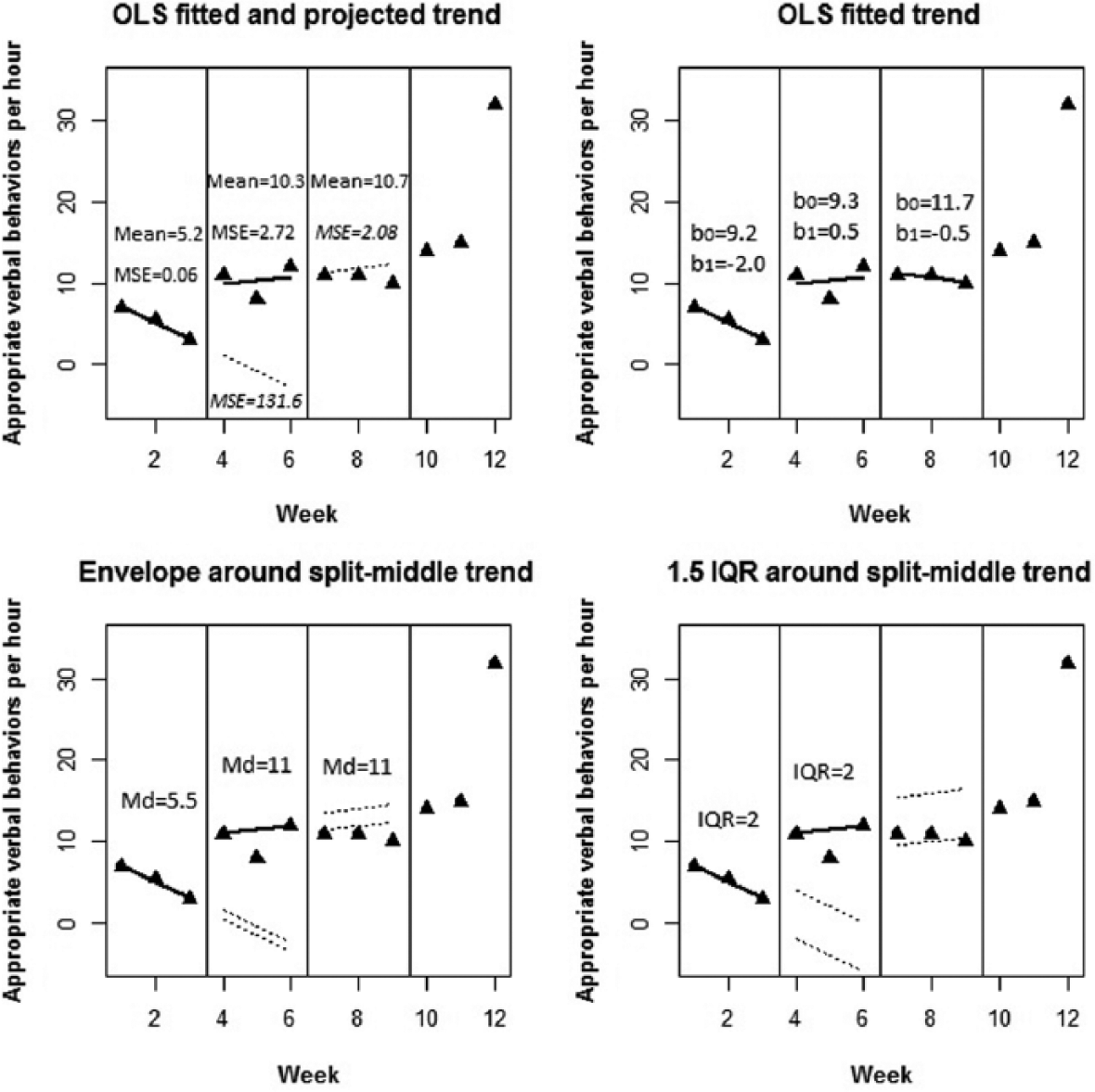
Data set reported by Petry et al. (1998) for the dispensary context: black triangles.

Simulated Data

Data generation: Design characteristics

The basic data series were simulated following two design structures: ABAB and MBD, both of which allow assessing functional relations (Kratochwill et al., 2010). The MBD is the most commonly used design (e.g., in 54% of the studies reviewed by Shadish & Sullivan, 2011, and 69% in the Smith, 2012, review). ABAB are also employed in single-case studies—in 8% of the studies reviewed by Shadish and Sullivan (2011) and 17% in Smith (2012). We focused on ABAB given that it presents certain analytical challenges in terms of the comparisons that need to be made. For instance, Scruggs and Mastropieri (1998) suggest performing comparisons that maintain the A-B sequence and Parker and Vannest (2012) also suggest that the B₁-A₂ comparison may have to be omitted as the behavior might not reverse fully to the initial level during the withdrawal (A₂) phase. On the other hand, Olive and Smith (2005) recommend comparing only the first baseline (A₁) and the last intervention phase (B₂). We decided to perform all three comparisons between adjacent phases, including the problematic B₁-A₂ comparison, to avoid the loss of information and to ensure that the ABAB design meets the criterion for including three attempts to demonstrate a functional relation (Kratochwill et al., 2010).

Regarding phase lengths, for the ABAB design, we specified n_A₁ = n_B₁ = n_A₂ = n_B₂ = 5, a recommended minimum per phase for rating highly the design according to Kratochwill et al. (2010). This data series length is in accordance with the characteristic of behavioral data: 20 measurements per design (median and modal value in the Shadish & Sullivan, 2011, review), 5 or more data points in the initial baseline phase (in more than half of the studies reviewed by the same authors), and an average of 11.69 baseline points (Smith, 2012). In addition, one of the conditions in this simulation study focused on phases with only three measurements (n_A₁ = n_B₁ = n_A₂ = n_B₂ = 3), given that we wanted to study the performance of the combining criteria and the effect size measures in a less favorable context (20% of the data sets had 3 data points in the A₁ phase in Shadish & Sullivan’s, 2011, review). This phase length is consistent with several standards for minimum phase length required (Chambless & Ollendick, 2001; Kratochwill et al., 2010). For the MBD design, we also used n_A = n_B = 5 for all three tiers to ensure that the conditions are comparable. For this design structure, we also studied the unfavorable conditions with n_A = n_B = 3, as was the case for ABAB designs. In addition, we included conditions with n_A = n_B = 10 in each tier, to include a broader set of conditions and to better approximate Smith’s (2012) finding of 10.40 baseline measurements on average in an MBD. This condition also makes the total amount of within-series data (20) equal for the ABAB and MBD and it matches previous simulation studies also using 10 initial baseline phase measurements (Smith, Borckardt, & Nash, 2012).

Data generation: Simulation model

Huitema and McKean’s (2000) model y_t = β₀ + β₁ · T_t + β₂ · D_t + β₃ · D_t · [T_t − (n_A+1)] + ε_t was used for generating data. With this model we specified (a) trend via the time variable T reflecting the session number; (b) level change via the dummy variable D set to 0 for the A phases and to 1 for the B phases; (c) slope change via the interaction between T and D, specifically using D_t · [T_t − (n_A + 1)]. For the error term (ε_t), we simulated either white noise (normal disturbance with mean zero and unitary standard deviation) or a first-order autoregressive process ε_t = ρ₁ · ε_t−1 + u_t for specifying different degrees of serial dependence.

We chose the simulation parameters on the basis of an empirical work to avoid arbitrary choices, although the data in any particular study cannot be considered representative of all SCED data. Specifically, in the present study we used Dolezal, Weber, Evavold, Wylie, and McLaughlin’s (2007) data on a participant called Mel (see Figure 2) for deciding the values of the level change and slope change parameters.

Figure 2.

Data gathered by Dolezal, Weber, Evavold, Wylie, and McLaughlin (2007) on a participant called Mel.

For level change, we took as a reference the first data set focused on percent on-task behavior, because the intervention was associated with an immediate and maintained shift in level. The median of the measurements of the A phases is 67.5 (used for β₀) and for the two B phases it is 100. Therefore, the level change (β₂) was set to 22.5. To include a condition with smaller effect, we divided this value by two, 11.25. The variability was also estimated from the data: as the standard deviation for the A₁ phase is 8.06 and for the A₂ 11.47, the median is 9.77 and so the value of 10 was chosen as a simulation parameter for the u_t variability.

For slope change we chose the data set representing words read per 2 min, provided that the effect can be conceptualized as a slope change, with the increase in the behavior becoming more prominent during the intervention. The intercept for the A₁ phase is 200 and for the A₂ phase it is 220; median equal to 210, which is the value for β₀. The slope for the A₁ phase is 7.5 and for the A₂ phase it is 8.5; median equal to 8 (and so β₁ = 8). The slope in the B₁ phase is 33.5 (a slope change of 33.5 − 7.5 = 26) and for the B₂ phase it is 22.5 (a slope change of 22.5 − 8.5 = 14); we took the median slope change 20 as a simulation parameter β₃. To represent a smaller effect, we divided this value by two. For taking into account level change in presence of baseline trend, we computed the immediate shift between the last baseline point and the first intervention point: for the A₁-B₁ comparison it was 16 and for A₂-B₂ 20, so we took 18 as a simulation parameter β₂. The variability was expressed in terms of standard deviation: 6.48 for A₁, 9.74 for A₂; a median of 8.11—after rounding 8 was used as simulation parameter for the u_t variability.

Data generation: Intervention effectiveness patterns

Different data patterns were simulated and they are represented in an idealized form (i.e., without the error variability) on Figure 3 for the ABAB design and on Figure 4 for the MBD, including the parameter values in the original and standardized metric. Pattern 1 includes no effect (i.e., β₀ = 67.5 and all other β parameters are equal to 0), whereas Patterns 2 and 4 include different magnitudes of change in level, β₂ = 11.25 and 22.5, respectively. Pattern 3 is the one representing a potentially undesirable situation—for ABAB an incomplete return to the baseline level in A₂ was simulated (β₂ = 22.5 for the A₁-B₁ difference, β₂ = 11.25 for the B₁-A₂ and A₂-B₂ differences). For the MBD, Pattern 3 is simulated as β₂ = 11.25, but for two of the three tiers the change in level is delayed (starting from the third instead of the first intervention phase measurement occasion). Patterns 5 and 6 are simulated with β₀ = 210 and different magnitudes of slope change, β₃ = 10 and 20, respectively. Pattern 7 includes no intervention effect, only general trend, β₁ = 8. Patterns 8 and 9 also include this trend, but a change in level (β₂ = 18) is present in Pattern 8 and a change in slope (β₃ = 10) in Pattern 9.

Figure 3.

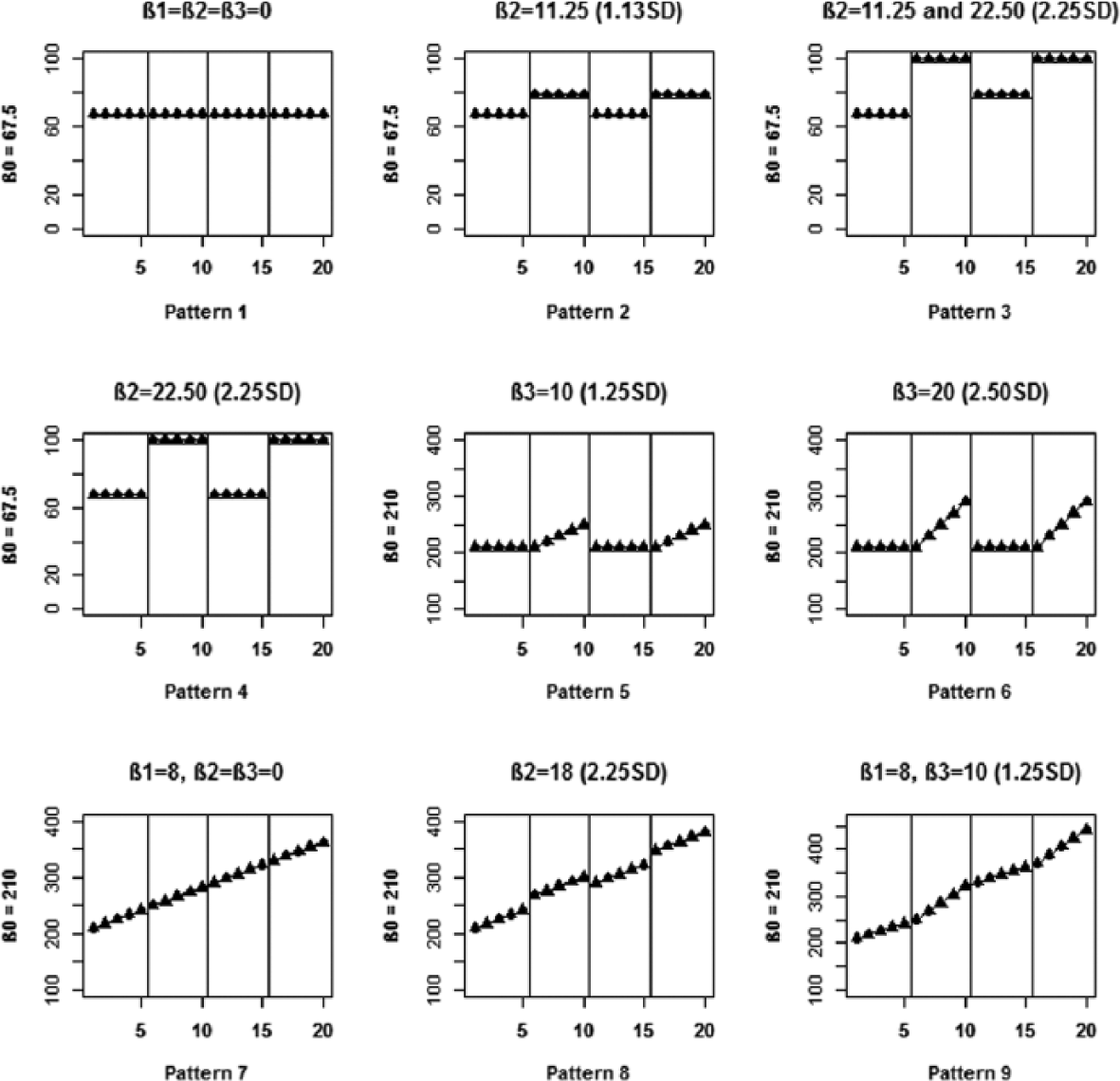
Simulated data patterns for the ABAB design in an idealized version (i.e., without the random variability).

Figure 4.

Simulated AB data patterns for the multiple-baseline design in an idealized version (i.e., without the random variability).

For the abovementioned patterns, the data were simulated to be uncorrelated. In addition, we studied the effect of autocorrelation focusing on data with no intervention effect or trend programmed (i.e., as in Pattern 1). Serial dependence (ϕ₁) was specified via the model ε_t = ϕ₁ · ε_t−1 + u_t, setting it either to 0 (independent data), .2 and .4 for the ABAB designs and .3 and .6 for MBD. The reason for choosing these values was the Shadish and Sullivan (2011) review in which the random effects bias-corrected meta-analytic mean was .191 (rounded here to .2) for reversal designs and .320 (rounded here to .3) for MBD. Thus, we included these degrees of autocorrelation and also twice these values to represent more extreme conditions. For each experimental condition, 1,000 data series were generated using R (R Core Team, 2013).

Simulation data analysis

For each data series generated for each experimental condition, we tallied the proportion of times that each criterion suggests a functional relationship is present. We wanted to explore how close the performance of the criterion would be to the desired 0% functional relations “detected” for Patterns 1 and 7 (with no effect simulated) and to the ideal 100% for the remaining ones. Given that it is not a priori straightforward to define the limits for what an acceptable or an unacceptable performance is, we decided to stick with the conventions followed in statistical significance testing (despite the fact that three of the four quantifications do not perform a test of statistical significance) to ensure an objective evaluation of the results. Thus, detection of inexistent functional relations ought to be as low as 5% of the iterations for Patterns 1 and 7. When studying the empirical Type I error rates in simulation studies, it is common to construct an interval of values considered to be acceptable. In that sense, we followed Bradley’s (1978) liberal criterion expressed as ± 0.5 times the reference value leading here to the range of acceptable values being [.025, .075]. We chose the liberal criterion, given that the quantifications do not actually entail a statistical significance test (except for RegCoeff) and thus we cannot talk properly about Type I errors.

On the other hand, following the usually employed benchmark for adequate statistical power (J. Cohen, 1992), the reference for acceptable detection of existing functional relations was chosen to be 80%. In this case, we used Bradley’s (1978) stringent criterion .80 ± 0.1(.80) leading to a range of [.72, .88]. We preferred the stringent to the liberal criterion to avoid labeling the 50% detection of existing effects as “appropriate.” It should be noted that this construction of intervals is consistent with Serlin’s (2000) proposal of using different criteria according the value around which the interval is constructed.

The results from the simulation study are presented in Tables 1 (ABAB design) and 2 (MBD). We will comment on these results separately after presenting each of the quantifications. Complementarily, the Discussion section includes an explicit comparison between the quantifications and some suggestions for modifying the quantifications that prove to perform better to increase their usefulness.

Table 1.

Proportion of Times Each of the Quantifications Suggests That a Functional Relation Is Presented in the Data for Each of the Nine ABAB Data Patterns With Independent Data and Five Measurements Per Phase and the Additional Conditions Tested.

Pattern	Parameter^a	MSE_M	RegCoeff	Env_Md	IQR_Md
1	None	.168	.105	.157	.095
2	β₂ = 11.25	.710	.188	.704	.507
3	β₂ = 22.50^b	.739	.306	.712	.562
4	β₂ = 22.50	.881	.505	.913	.739
5	β₃ = 10.00	.980	.688	.493	.900
6	β₃ = 20.00	1.000	1.000	.983	1.000
7	β₁ = 8.00	0	.977	0	0
8	β₁ = 8.00, β₂ = 18.00	0	.863	0	0
9	β₁ = 8.00, β₃ = 10.00	0	.988	0	0
ϕ = .2	None	.156	.148	.171	.121
ϕ = .4	None	.168	.212	.179	.142
n_i = 3	None	.156	.193	.193	.144
n_i = 3	β₂ = 22.50	.894	.400	.917	.709
n_i = 3	β₃ = 20.00	.988	.535	.700	.894

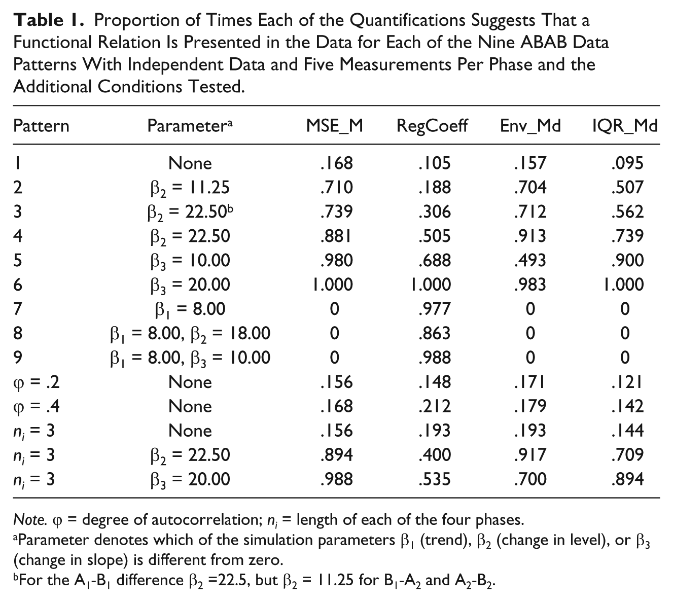
Note. ϕ = degree of autocorrelation; n_i = length of each of the four phases.

Parameter denotes which of the simulation parameters β₁ (trend), β₂ (change in level), or β₃ (change in slope) is different from zero.

For the A₁-B₁ difference β₂ =22.5, but β₂ = 11.25 for B₁-A₂ and A₂-B₂.

Table 2.

Proportion of Times Each of the Quantifications Suggests That a Functional Relation Is Presented in the Data for Each of the Nine Multiple-Baseline Data Patterns With Independent Data (ϕ = 0, Unless Stated Otherwise) and Five (Upper Part), Ten (Middle Part), or Three (Lower Part) Measurements Per Phase.

Pattern	Parameter^a	MSE_M	RegCoeff	Env_Md	IQR_Md
1	None	.086	.085	.104	.071
2	β₂ = 11.25	.694	.264	.696	.516
3	β₂ = 11.25^b	.555	.121	.512	.363
4	β₂ = 22.50	.909	.519	.931	.742
5	β₃ = 10.00	1.000	.700	.319	.867
6	β₃ = 20.00	1.000	1.000	.972	.995
7	β₁ = 8.00	.746	.995	.016	.055
8	β₁ = 8.00, β₂ = 18.00	.905	1	.161	.723
9	β₁ = 8.00, β₃ = 10.00	.973	.998	.312	.402
ϕ = .3	None	.099	.159	.105	.081
ϕ = .6	None	.095	.231	.099	.090
1	None	.088	.047	.123	.083
2	β₂ = 11.25	.766	.298	.928	.678
3	β₂ = 11.25^b	.733	.136	.882	.665
4	β₂ = 22.50	.949	.869	.992	.793
5	β₃ = 10.00	1.000	1.000	.998	.999
6	β₃ = 20.00	1.000	1.000	1.000	1.000
7	β₁ = 8.00	.659	1.000	.030	.001
8	β₁ = 8.00, β₂ = 18.00	.945	1.000	.136	.010
9	β₁ = 8.00, β₃ = 10.00	1.000	1.000	.973	.650
ϕ = .3	None	.100	.138	.118	.090
ϕ = .6	None	.088	.285	.111	.086
n_i = 3	None	.106	.153	.121	.093
n_i = 3	β₂ = 22.50	.898	.360	.921	.755
n_i = 3	β₃ = 20.00	.982	.521	.616	.845

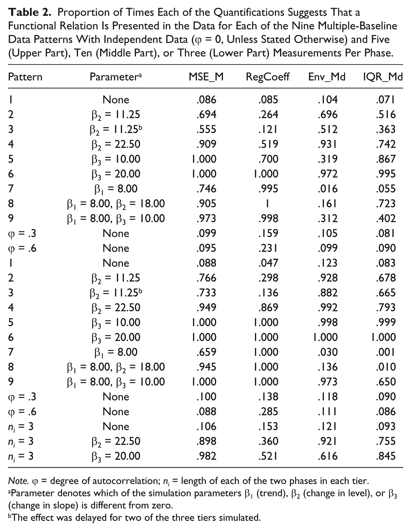
Note. ϕ = degree of autocorrelation; n_i = length of each of the two phases in each tier.

Parameter denotes which of the simulation parameters β₁ (trend), β₂ (change in level), or β₃ (change in slope) is different from zero.

The effect was delayed for two of the three tiers simulated.

Quantifications

Quantification 1: MSE_M

Rationale

The first quantification is referred to as MSE_M, given that it includes computing mean square error (MSE)¹ and the mean in each phase. This quantification is based on estimating ordinary least squares (OLS) baseline trend and projecting it into the intervention phase. We chose OLS instead of generalized least squares (GLS; Maggin et al., 2011) as OLS is more straightforward and potentially more easily understood and applicable via mainstream statistical packages and GLS presents the unsolved issue of the optimal estimation of autocorrelation (Solanas, Manolov, & Sierra, 2010). According to the proposal, a functional relation is demonstrated when the MSE of the baseline measurements around the baseline trend is smaller than the MSE of the intervention measurements around the baseline trend’s projection into the treatment phase. We chose the MSE instead of the mean absolute error (Hyndman & Koehler, 2006), given that the former is more well-known. The second criterion is that the mean of the intervention measurements should be greater than the mean of the baseline measurements (assuming an improvement is represented as an increase in the behavior of interest). Finally, the quantification that could be used for weighting effect sizes is the inverse of the MSE in the baseline phase (or, in general, of the phase whose data are used for fitting the regression line), given that the predictability of the baseline is directly related to its usefulness as a reference for all further comparisons.

Illustration with real behavioral data

An OLS regression line (b₀ = $9.1 \overset{⌢}{6}$ and b₁ = −2) fitted to the A₁ measurements can be projected into the B₁ phase. We see that the predicted values are lower than the ones actually obtained, given the decreasing trend present in A₁ and the shift in level in B₁. The MSE around the regression line fit in A₁ is $0.0 \overset{⌢}{5}$ whereas the MSE around the projected phase B slope (using the coefficients estimated in A₁) is 131.6, plus the B₁ mean (10.33) is greater than the A₁ mean (5.17). Thus, we have quantitative evidence that the A₁ trend does not predict well the B₁ data and, therefore, there has been a change in the behavior with the change in phase. The regression line (b₀ = 9.3 and b₁ = 0.5) fitted to the B₁ data, when projected into the next phase, approximates well the A₂ data, given that there is practically no change in level or slope. The MSE for B₁ is 2.72, whereas for the predicted A₂ measurements (using the coefficients estimated in B₁) it is 2.08. Thus, we have numerical evidence that there is no change in the behavior. Therefore, a functional relation cannot be demonstrated and the final comparison (A₂-B₂) will not be made.

A priori advantages and limitations

The advantages of this quantification are (a) it is potentially well-understood by applied researchers accustomed to using common parametric statistical methods; (b) it avoids making a statistical decision regarding whether a functional relation has been demonstrated, given that a statistical significance test might be misunderstood as a necessary step for computing or reporting an effect size. The main limitation is that when the two MSEs are compared, it might be necessary to specify a cut-off point for labeling the difference as either relevant or irrelevant; any such choice is potentially arbitrary.

Simulation evidence regarding its performance

First, we comment on the performance of the quantification in the absence and in the presence of effect, for data patterns without trend or autocorrelation. For the ABAB design, in absence of effect there is an excessively high amount of false positives (i.e., an indication of the existence of effect when such has not been simulated), whereas for the MBD the false positive rates are approximately adequate. When there is an effect expressed as change in level simulated, for both the ABAB design and the MBD, MSE_M is one of the quantification with highest detection rate (close to 80% of the cases). The two magnitudes of change in slope simulated were detected practically always by this quantification. The detection of change in level is affected for incomplete return to baseline levels in the A₂ phase (ABAB design) and delayed effects (MBD). Next, we discuss the effect of trend on the quantification. For both ABAB designs, in absence of intervention effect, trend has only slight influence on the performance of MSE_M, but in presence of effect it is affected, due to the criterion requiring the B₁ mean to be greater than the A₂ mean. For MBD, trend distorts the performance of MSE_M even in absence of effect. Regarding the effect of autocorrelation, the performance of this quantification was not distorted. Regarding the influence of phase length, for both design structures, shorter phase lengths (n_i = 3) are not related to higher false positive rates only for this quantification. For ABAB designs, the detection of change in level or change in slope is generally not affected (comparing n_i = 3 to n_i = 5). For MBD, the change in level or in slope is more frequently detected in the longer series, whereas the (absence of) effect of autocorrelation is practically the same for phases with 5 or 10 measurements.

Quantification 2: RegCoeff

Rationale

The second quantification is referred to as RegCoeff, because it includes an estimation and comparison of intercept and slope coefficients in the context of regression analysis. Thus, the regression lines fitted in the two contiguous phases are compared statistically, following A. Cohen’s (1983) large-sample formula for contrasting the difference between slope coefficients without assuming homoscedasticity. The expression used for computing the tstatistic was $(b_{1} - b_{12}) / \sqrt{\frac{{\hat{σ}}_{12}}{S S_{X 1}} + \frac{{\hat{σ}}_{22}}{S S_{X 2}}}$ , where b₁ and b₂ are theslope coefficients in the two regression models (one for the first phase and one for the second one), the ${\hat{σ}}^{2}$ are the variances of the residuals in these phases, and SS_X are the sums of squares of the predictors (i.e., the variables representing time in this case); $S S_{X} = \sum_{i = 1}^{n} {(x_{i} - \bar{x})}^{2}$ .

For comparing the intercepts (i.e., assessing a potential change in level), after controlling for trend, we carried out analysis of covariance (ANCOVA) as suggested by A. Cohen (1983). We first estimated the slope coefficients (separately in each phase) and then obtained the predicted measurements using the following expression ${\hat{y}}_{1} = b_{0} - b_{1} T i m e_{i}$ , with Time being the variable representing measurement occasion (1, 2, …, n) and b₀ = 0 to maintain any differences in intercept. Afterwards, the residuals were obtained, once again separately for each phase. To compare statistically these intercepts or average levels, we performed analysis of variance (ANOVA) to the residuals.

The criterion for identifying functional relation was based on the two statistical tests: there should either be statistically significant difference between the slope coefficients (change in slope) in all two-phase comparisons using the t distribution with n_A + n_B − 4 degrees of freedom² or the result of the ANOVA on the detrended data should be statistically significant (change in level). Finally, the quantification that could be used for weighting effect sizes is the inverse of the MSEs around the regression lines fit to both phases being compared, given that more clear patterns offer greater certainty about the existence or lack of effect.

Illustration with real behavioral data

The OLS regression coefficients estimates separately for the A₁ phase (b₀ = $9.1 \overset{⌢}{6}$ , b₁ = −2) and the B₁ phase (b₀ = 9.3, b₁ = 0.5) are comparing yielding t = 1.73, a value that is smaller than the one-tail 5% cut-off value of for the t distribution with n_A + n_B − 4 = 2 degrees of freedom, t_0.05 = 2.92. Thus, the slope change is not statistically significant, probably due to low power related to the short phases. To test for a difference in intercepts, the detrended measurements are obtained (9, 9.5, and 10 for phase A₁ and 10.5, 7, and 10.5 for B₁) and compared via ANOVA: F(1, 4) = 0.02, p = .894. Thus, the change in level (after controlling for within-phase trends) is not statistically significant. As there is no statistically significant change already for the first two-phase comparison, a functional relation cannot be demonstrated and the other two comparisons (B₁-A₂ and A₂-B₂) will not be made.

A priori advantages and limitations

The advantages of this quantification are as follows: (a) the decision of a functional relation is based on a commonly used significance testing with a conventional nominal significance of .05 and (b) the comparison is made between two trends fitted to two different sets of data which avoids the problem of any unrealistic projections of baseline trends (Parker et al., 2011). The limitations of this quantification are (a) the logic of the comparison is based on group designs and independent data with normally distributed residual and (b) before any further evidence is obtained, the formulae and the t test are only asymptotically correct for the purpose intended here.

Simulation evidence regarding its performance

Quantification 3: Env_Md

Rationale

The third quantification is referred to as Env_Md, given that it includes constructing a stability envelope around a trend line, estimated nonparametrically, and comparing the median in each phase. For estimating trend, we chose the well-known split-middle method (White, 1972) used in visual analysis. Trend stability is assessed as suggested by Gast and Spriggs (2010), following the idea of an “envelope” with limits defined by 10% of the value of the median. According to the 80%─20% formula, if less than 80% of the data in the subsequent phase fall within the projected “envelope,” then there is evidence that a change has occurred. We decided not to use the binomial test associated with the split-middle method, given the unfavorable evidence available (Crosbie, 1987). The second criterion, related to the level of behavior, was that the intervention phase median should be greater than the baseline median (assuming an improvement is an increase in the behavior of interest). Finally, the quantification that could be used for weighting effect sizes is the proportion of measurements in the baseline phase (or, in general, in the phase whose data is used for fitting the split-middle trend line) that fall within the trend envelope, given that predictable data are considered to be crucial for any further comparisons.

Illustration with real behavioral data

The split-middle trend line (including the values 7, 5, and 3) in the A₁ phase was projected into phase B. The median of the A₁ phase is 5.5 and within the limits defined by ± 10% (5.5) none of the B₁ values are contained. Moreover, the B₁ median (11) is greater and, thus, there is evidence of a behavioral change. The B₁ split-middle trend line (11, 11.5, and 12) is then projected into A₂ with the limits defined from the B₁ median and, once again, less than 80% of the A₂ measurements are included. However, in this case, the A₂ median (11) is not smaller than the B₁ median and thus the second criterion is not met, which suggests that there is no behavioral change. Therefore, a functional relation cannot be demonstrated and the final comparison (A₂-B₂) will not be made.

A priori advantages and limitations

The advantages of this quantification are (a) it is potentially well-understood by applied researchers accustomed to using visual analysis and visual aids and (b) it avoids making a statistical decision. The main limitation of this quantification is that the 80%─20% formula is objective, but it is still arbitrary. Specifically, the rule does not consider the actual variability in the phase in which the trend line is estimated.

Simulation evidence regarding its performance

First, we comment on the performance of the quantification in the absence and in the presence of effect, for data patterns without trend or autocorrelation. For both the MBD and ABAB design, in the absence of effect there is an excessively high amount of false positives.

Second, when there is an effect expressed as change in level simulated, for both the ABAB design and the MBD, Env_Md is one of the quantification with highest detection rate: greater than 70% to 90% for the effects simulated. In contrast, change in slope Env_Md is the quantification that proves to be least sensitive for both design structures: it only reaches the .80 detection rate only for the larger effect (β₃ = 20). The detection of change in level is affected for incomplete return to baseline levels in the A₂ phase (ABAB design) and delayed effects (MBD).

A third focus of attention is the effect of trend on the quantification. For both design structures, in absence of intervention effect, trend actually makes Env_Md more conservative, which is translated into null detection of effects in ABAB designs it is affected, due to the criterion requiring the B₁ median to be greater than the A₂ median. For the MBD, trend in presence of change in level affects Env_Md more than the other procedures, probably due to the fact that a large median (greater than 200) leads to broader limits and more difficulty in detecting effects. Regarding the effect of autocorrelation, the performance of this quantification was not affected for MBD, with distortion being somewhat more notable, but not excessive, for ABAB designs. Regarding the influence of phase length, for both design structures, shorter phase lengths (n_i = 3) are related to higher false positive rates. For ABAB designs, the detection of change in level is generally not affected (comparing n_i = 3 to n_i = 5) due to shorter series, but the detection of change in slope is affected. For MBD, the change in level or in slope is more frequently detected in the longer series, whereas the (absence of) effect of autocorrelation is practically the same for phases with 5 or 10 measurements.

Quantification 4: IQR_Md

Rationale

The fourth quantification is referred to as IQR_Md, given that it includes constructing the limits around a split-middle trend line on the basis of the interquartile range and computing the median in each phase. Hence, here the limits around the trend line are computed considering the variability in the data, instead of using a fixed a priori criterion as in Env_Md. Variability here is estimated using a resistant index such as the interquartile range (IQR); specifically, the limits are constructed subtracting and adding 1.5 times the IQR to the trend line. The same rule is used in exploratory data analysis (Tukey, 1977) in the context of the construction of the boxplot for identifying outliers. For this quantification, the criterion was that at least one of the measurements of the subsequent phase should not fall within the limits established considering the previous phase trend and variability. The second criterion, related to the level of behavior, was that the intervention phase median should be greater than the baseline median (assuming an improvement is an increase in the behavior of interest). Finally, the quantification that could be used as a weight for effect sizes is the inverse of the IQR of the baseline phase measurements (or, in general, of the phase whose data are used for fitting the split-middle trend line), given the importance of stable data for any further comparisons.

Illustration with real behavioral data

The split-middle trend line (with values 7, 5, and 3) in the A₁ phase, when projected into B₁ with limits defined by ± 1.5 IQR (equal to 2), does not contain any of the B₁ values.³ Moreover, the B₁ median is greater than the A₁ median (11 vs. 5.5) and, thus, there is evidence of a behavioral change. The B₁ split-middle trend line (11, 11.5, and 12) with its limits is then projected into A₂ considering that the IQR for the B₁ measurements is also equal to 2. In this case, 66.66% of the A₂ measurements are included meeting the first criterion, but the equal medians go against the second criterion. Therefore, a functional relation cannot be demonstrated and the final comparison (A₂-B₂) will not be made.

A priori advantages and limitations

The advantages of this quantification are (a) it is potentially well-understood by applied researchers accustomed to using visual analysis and visual aids and (b) it avoids making a statistical decision. The main limitation of this quantification is that the 1.5 IQR rule is originally intended for detecting outliers and not for building limits around trend in time. In addition, one could argue that the 3 IQR rule also used in the boxplot for identifying extreme outliers could have been used instead.

Simulation evidence regarding its performance

First, we comment on the performance of the quantification in absence and in presence of effect, for data patterns without trend or autocorrelation. For the ABAB design, in absence of effect, IQR_Md is one of the quantifications performing better, but still beyond the .075 upper limit of appropriate performance. For the MBD, the false positive rates are approximately adequate. When there is an effect expressed as change in level simulated, for both the ABAB design and the MBD, the performance of IQR_Md in terms of detection of effects is in the middle of the remaining quantifications, but closer to the best performers than to RegCoeff. The two magnitudes of change in slope simulated were detected practically always by this quantification. The detection of change in level is affected for incomplete return to baseline levels in the A₂ phase (ABAB design) and delayed effects (MBD). Next, we discuss the effect of trend on the quantification. For both design structures, in absence of intervention effect, trend actually reduces the false positives for IQR_Md, which is reflected in suboptimal detection of existing effects in ABAB designs, due to the criterion requiring the B₁ median to be greater than the A₂ median. Trend in presence of change in slope affects mostly the IQR_Md, given that for shorter series (n_i = 5) an intervention point out of the IQR limits is only obtained for abrupt changes (in level) and for longer series (n_i = 10) this is achieved only when the change is progressive (i.e., slope change). Regarding the effect of autocorrelation, the performance of this quantification was only slightly affected for MBD, whereas the distortion is more notable for ABAB designs. Regarding the influence of phase length, for both design structures, shorter phase lengths (n_i = 3) are related to higher false positive rates. For ABAB designs, the detection of change in level or change in slope is generally not affected (comparing n_i = 3 to n_i = 5). For MBD, the change in level or in slope is more frequently detected in the longer series, whereas the (absence of) effect of autocorrelation is practically the same for phases with 5 or 10 measurements.

Free Software Resources for Applied Researchers

Our aim with the current article was not only to discuss how visual analysis and additional quantifications can aid the assessment of functional relations in behavior modification programs; we rather intended to offer applied researcher a practical tool with a logical basic, straightforward to understand and easy to implement. This is why in the present section we offer code (or syntax) for the open-source software R, explaining its use in a step-by-step fashion. We have focus on the two quantifications: IQR_Md and Env_Md. IQR_Md proved to perform best in the simulation conditions studied distinguishing between data with and without effect and proving to be undistorted by autocorrelation or trend in some cases. Nevertheless, as we discuss later, this quantification is not flawless given the problematic performance for some data patterns and can be improved in future studies. Env_Md was included in the code to enable researchers to use it as a visual aid based on resistant and nonparametric statistics, not as a quantification.

The first step is to install R, which can be freely downloaded from http://cran.r-project.org, choosing the operating system used. The second step is to download the R code, which is also available, as provided by the first author (R.M.), free of charge from the following URL https://www.dropbox.com/s/3t2e92fejju4tuv/ProjectTrend_Weight.R. This code can be opened and modified with a simple text processing program such as Notepad. The code contains an initial PART 0 with copyright information and references (all lines preceded by the symbol #). The subsequent PART 1 is actually the first one to be read and executed by R. Immediately after the line stating “Input data” a string of data is entered by default, but they can easily be changed substituting the values available by the researcher’s own value. Here we illustrate how to do this with the Ganz et al. (2012) data⁴ on making questions as a communicative behavior exhibited by a participant called Debby and labeled as a typically developed student. The first line of the “Input data” section is only descriptive and need not be changed. The second line contains that the data points separated by commas and the third part denotes the baseline phase length.

# Input data

score <- c(74.92,91.95,91.02,100,66.56,100, 91.64,74.92,74.92,66.56,83.28,74.92,74.92,91.64,58.20,83.28,58.20,41.48,58.20,41.48)

n_a <- 6

PART 2 of the code includes some options that can be changed, if desired. By default, the 20% of the median is used to construct the envelope, but this value can be modified changing the number after “md_percentage <- .” The rule for constructing the IQR limits can also be changed from the default 1.5 changing the value after “IQR_value <- .” PART 3 of the code needs not be changed. Therefore, after inputting the data (compulsory) and changing the values for the quantifications (optional, especially given that the values by default have already been used in statistics), all the code is copied and pasted into the R console. The results of this copy-paste operation are several. First, a graphical representation is obtained, as shown on Figure 5.

Figure 5.

Graphical representation of the Ganz et al. (2012) data on the making questions behavior of a participant called Debby.

Second, information is provided regarding the use of the quantifications, Env_Md and IQR_Md, as one of the pieces of evidence in the assessment of functional relations. Note that only IQR_Md is used as an indicator of functional relations, whereas Env_Md is used as a visual aid and thus makes no suggestion regarding whether there is a change in the behavior.

“Percentage of phase B data into envelope”

“Percentage of phase B data into IQR limits”

7.14

“The IQR limits suggest change in the behavior”

Third, the information about the medians is provided, but it is not interpreted in relation to the functional relation, considering the comments provided later in the Discussion about some of the data patterns.

“The median of the first phase” 91.485 “is greater than the median of the second phase” 74.92

Fourth, the weight for subsequent meta-analyses is provided for IQR_Md, the only of the procedures that the simulation supports as a potentially useful tool for aiding the assessment of functional relation. Note that this weight can only be meaningfully interpreted when comparing the current data to other data sets with more or less variable baselines.

“Weight according to the IQR limits: Inverse of the baseline interquartile range”

0.0525

This illustration shows how the quantifications can be used as additional evidence when assessing functional relations. Moreover, the example shows that it is important to consider the logical or natural limits of the behavior when projecting trends (i.e., what is the meaning of a percentage greater than 100?), an issue discussed by Parker et al. (2011). Finally, with the current code we aim to encourage publishing at least the graphical representation of the data so that it is made available for future meta-analyses, alongside the quantitative information that can be useful for the same aim. The visual aids added to the graphed data can also be used as objective tools in the process of visual analysis.

Discussion

Summary of the Simulation Evidence: Comparison Between the Quantifications

In the current simulation study, we studied the performance of four quantifications intended to add an objective criterion to the visual assessment of functional relations. Data were simulated for two design structures, ABAB and MBD, for a variety of data patterns. Figure 6 provides a flowchart that can be used as a summary of the results, on the basis of two premises: (a) it is first necessary that the quantification does not detect “excessively frequently” inexistent effects, before assessing its capacity to detect “frequently enough” existing effects and (b) Bradley’s liberal criterion⁵ is used for defining the .075 value that marks what “excessively frequently” is, whereas Bradley’s stringent criterion is employed for defining the minimal detection rate of .72 considered to be “frequently enough.”

Figure 6.

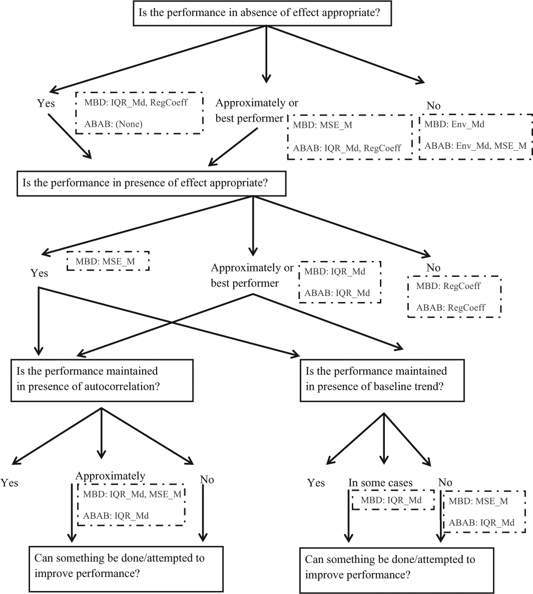
Flowchart for assessing the performance of the quantifications, choosing among them or introducing modifications.

First, the relative frequency of times that the quantifications (except Env_Md and MSE_M for ABAB designs) suggest that there is a functional relationship in absence of effect is not excessive considering the high false positive rates reported for visual analysts (Matyas & Greenwood, 1990; Normand & Bailey, 2006). Second, the reasonably high detection rates reported here should be assessed in the light of the relatively short (but potentially common) phases. In general, following the flowchart for the best performers for MBD were MSE_M and IQR_Md. However, their performance is not optimal in terms of autocorrelation. Whereas for the MSE_M a GLS estimation could be useful for dealing with this problem (e.g., Maggin et al., 2011), for IQR_Md no clear alternative is directly discernible.

For the ABAB design, the best performer was IQR_Md, but it did not detect effects in presence of trend (i.e., Patterns 8 and 9). Our conjecture was that this is due to the criterion related to the median, specifically, due to the fact that the A₂ median is higher than the B₁ median. We modified the median criterion (now being “or” instead of “and,” in the same way as it is for RegCoeff, and the result was that IQR_Md improved the detection of change in level [.893] and change in slope [.661]). (Similar results were obtained for MSE_M and Env_Md as the mean and median criteria were modified for these data patterns.) When we performed this check, we simulated an additional data pattern with decreasing trend (β₁ = −10) followed by a positive slope change (β₃ = 20) leading to an increasing trend with no change in the average value. The performance of the modified version of IQR_Md was also adequate (a detection rate of .993) for this additional data pattern.

For the MBD, as a strategy to attempt solving the IQR_Md problems for detecting existing effects in presence of trend, it is possible to use the IQR as computed for the residuals around the trend line, instead of the IQR for the data, as they are not stationary. The additional simulations we performed to test this solution show that the 1.5 IQR around the trend line is too liberal, whereas 3 IQR rule (also used in exploratory data analysis) worked better than the original version only for 10 measurement phases (.082 detection rate for no effect, .224 for level change, and .950 for slope change) but not for 5-phase measurements (.133 detection rate for no effect, .308 for level change, and .513 for slope change).

The need for a posteriori modifications suggest that the quantitative criteria should always be used jointly with visual analysis to validate their results (Parker, Cryer, & Byrns, 2006) and to improve the decisions made regarding the functional relation between intervention and behavior. However, it should be kept in mind that these two pieces of information (visual and quantitative) need to be considered in the light of the way in which the conditions were manipulated and the behavior was reinforced or punished, and the potential influence of any external factors on the behavior of interest, before reaching any firm conclusion on the existence of a functional relation.

Implications of the Results

A finding common to all quantifications is that Pattern 3 (incomplete reversal to baseline levels in ABAB and delayed effect in MBD) is actually problematic for detecting the presence of an effect quantitatively. This adds evidence to the previous debate on whether the B₁-A₂ comparison has to be taken into account or its inclusion maybe more problematic than informative. A second finding is that the IQR_Md shows reasonable performance for detecting functional relations and, unlike randomization tests and visual aids, the quantification it entails (specifically, the baseline phase variability) can be used when weighting effect sizes in meta-analytical integrations. In the following paragraphs we propose how the information regarding functional relations can be used in meta-analysis, given that it might not be warranted to assume that larger effects necessarily imply functional relations.

We do not advocate for reporting or including in meta-analyses only effect sizes pertaining to studies with demonstrated functional relation, because such an approach might lead to the dichotomous thinking that undermines the use of p values (J. Cohen, 1994; Nickerson, 2000). Given that statistical decision making (i.e., to reject or not the null hypothesis) on the basis of p values has been criticized for precluding the assessment of the strength of evidence on a continuous scale (Nickerson, 2000), it would not be appropriate to repeat the same practice when assessing functional relations. Instead, the researcher’s judgment on whether a functional relation is present has to be complemented by the estimation of the magnitude of effect, which would quantify the strength of the evidence.

One option would be to follow an approach similar to vote-counting and tallying the proportion of studies included in a meta-analysis for which a functional relation is demonstrated. This information can be used as a complement to (and not a substitute for) the effect size calculation (Bushman & Wang, 2009). However, in the case of SCED, vote-counting would not depend on the statistical significance of the result, but on whether a functional relation is judged to be present or not.

Another option would be to give weights to the effect size, using some meaningful and easily available quantity. We propose that this quantity be related to the quantification used for assessing the existence of a functional relation. However, until an appropriately functioning quantification for all data patterns is identified, it might be premature to point at the most appropriate weight. Nonetheless, we can give some indications on weighting strategies in SCED. Specifically we consider that the weight should be related to baseline stability, given the importance of the baseline as a reference for all further comparisons (Kazdin, 2013; Smith, 2012). Moreover, baseline stability is a requirement for the proper functioning of multilevel models used for meta-analysis (Owens & Ferron, 2012) and the type of stability in the data (e.g., stability around an increasing trend; Hedges et al., 2012) is relevant for choosing the appropriate type of quantification. This idea is well-aligned with a recent proposal for weighting on the basis of the baseline length and variability (Manolov, Guilera, & Sierra, 2014). Nevertheless, it is still debatable which the optimal operative definition of baseline variability (e.g., robust coefficient of variation) is and whether variability of the data or variability of the residuals around a trend line should be considered.

Limitations and Future Research

The limitations of the simulation study refer to the necessarily limited set of conditions studied in terms of phase lengths and magnitudes of effect. In that sense, the relative frequency with which functional relations are detected is clearly related to magnitude of behavioral change (i.e., the β₂ and β₃ parameters). Furthermore, the simulation was performed using continuous data (i.e., normal random disturbance) as it is commonly done (e.g., Beretvas & Chung, 2008; Ugille, Moeyaert, Beretvas, Ferron, & Van den Noortgate, 2012), but in SCED, discrete measures of frequency of the target behavior are common (e.g., a Poisson model could be useful).

We hope that the current article will contribute to the discussion on how functional relations should be assessed in the context of single-case studies. On one hand, it is relevant to know whether the recommendations of academics and methodologists regarding visual analysis are well-aligned with actual practice and with the predisposition of applied researchers to change their way of treating the data. In that sense, we ask ourselves the following: Do practitioners consider that visual inspection used exclusively is sufficient or it can benefit from quantitative evidence? On the other hand, the answer of this question is probably related to the amount of time and training required for implementing quantitative analysis and visual aids. Thus, the second question is as follows: Are applied researchers willing to copy-paste R code to represent graphically their data alongside visual aids and quantifications? A third aspect that requires debate is whether quantitative integrations need to consider only the size of the effect or also the degree of evidence on its likely cause. In case the information about functional relations is considered to be important, the question is How can this information be included in meta-analyses? Do researchers consider the vote-counting approach to be appropriate? Furthermore, the option for weighting has to be discussed in comparison with the inverse of the effect size index variance as a possible gold standard, as it is in group-design studies (Borenstein, 2009), with recent developments also in the context of single-case studies (Hedges et al., 2012, 2013).

Footnotes

Declaration of Conflicting Interests

The author(s) declared no potential conflicts of interest with respect to the research, authorship, and/or publication of this article.

Funding

The author(s) received no financial support for the research, authorship, and/or publication of this article.

Notes

Author Biographies

Rumen Manolov, PhD, is assistant lecturer at the Faculty of Psychology at the University of Barcelona and visiting research at the ESADE Business School, Ramon Llull University in Spain. His investigation is focused on single-case designs data analysis.

Vicenta Sierra, PhD, is associate professor at the ESADE Business School, Ramon Llull University, Spain. Her research is focused on single-case data analysis and, more recently, it deals with the analysis of social systems, human resource management, group dynamics, and interpersonal perception.

Antonio Solanas, PhD, is professor at the Faculty of Psychology at the University of Barcelona, Spain. His main research interests include single-case designs analysis, social reciprocity measurement, and multivariate data analysis methods.

Juan Botella, PhD, is professor at the Faculty of Psychology, Autonomous University of Madrid, Spain. His methodological research deals with meta-analysis, while more applied research areas include human attention and evaluation and personnel selection.

References

APA Presidential Task Force on Evidence-Based Practice. (2006). Evidence-based practice in psychology. American Psychologist, 61, 271-285.

Arnau

Bono

(2001). Autocorrelation and bias in short time series: An alternative estimator. Quality & Quantity, 35, 365-387.

Bailey

D. B.

(1984). Effects of lines of progress and semilogarithmic charts of ratings of charted data. Journal of Applied Behavior Analysis, 17, 359-365.

Barlow

D. H.

Nock

M. K.

Hersen

(2009). Single case experimental designs: Strategies for studying behavior change (3rd ed.). Boston, MA: Pearson.

Beretvas

S. N.

Chung

(2008). An evaluation of modified R2-change effect size indices for single-subject experimental designs. Evidence-Based Communication Assessment and Intervention, 2, 120-128.

Borenstein

(2009). Effect sizes for continuous data. In Cooper

Hedges

L. V.

Valentine

J. C.

(Eds.), The handbook of research synthesis and meta-analysis (2nd ed., pp. 221-236). New York, NY: Russell Sage.

Bradley

J. V.

(1978). Robustness? British Journal of Mathematical and Statistical Psychology, 31, 144-152.

Brossart

D. F.

Vannest

K. J.

Davis

J. L.

Patience

M. A.

(2014). Incorporating nonoverlap indices with visual analysis for quantifying intervention effectiveness in single-case experimental designs. Neuropsychological Rehabilitation, 24, 464-491.

Bushman

B. J.

Wang

M. C.

(2009). Vote-counting procedures in meta-analysis. In Cooper

Hedges

L. V.

Valentine

J. C.

(Eds.), The handbook of research synthesis and meta-analysis (2nd Ed., pp. 207-220). New York, NY: Russell Sage.

10.

Carter

(2009). Effects of graphing conventions and response options on interpretation of small n graphs. Educational Psychology, 29, 643-658.

11.

Chambless

D. L.

Ollendick

T. H.

(2001). Empirically supported psychological interventions: Controversies and evidence. Annual Review of Psychology, 52, 685-716.

12.

Cohen

(1983). Comparing regression coefficients across subsamples: A study of the statistical test. Sociological Methods & Research, 12, 77-94.

13.

Cohen

(1992). A power primer. Psychological Bulletin, 112, 155-159.

14.

Cohen

(1994). The earth is round (p < .05). American Psychologist, 49, 997-1003.

15.

Crosbie

(1987). The inability of the binomial test to control Type I error with single-subject data. Behavioral Assessment, 9, 141-150.

16.

Danov

S. E.

Symons

F. J.

(2008). A survey evaluation of the reliability of visual inspection and functional analysis graphs. Behavior Modification, 32, 828-839.

17.

Davis

D. H.

Gagné

Fredrick

L. D.

Alberto

P. A.

Waugh

R. E.

Haardörfer

(2013). Augmenting visual analysis in single-case research with hierarchical linear modeling. Behavior Modification, 37, 62-89.

18.

DeProspero

Cohen

(1979). Inconsistent visual analyses of intersubject data. Journal of Applied Behavior Analysis, 12, 573-579.

19.

Dolezal

D. N.

Weber

K. P.

Evavold

J. J.

Wylie

McLaughlin

T. F.

(2007). The effects of a reinforcement package for on-task and reading behavior with at-risk and middle school students with disabilities. Child & Family Behavior Therapy, 29, 9-25.

20.

Fisch

G. S.

(2001). Evaluating data from behavioral analysis: Visual inspection or statistical models? Behavioural Processes, 54, 137-154.

21.

Fisher

W. W.

Kelley

M. E.

Lomas

J. E.

(2003). Visual aids and structured criteria for improving visual inspection and interpretation of single-case designs. Journal of Applied Behavior Analysis, 36, 387-406.

22.

Gage

N. A.

Lewis

T. J.

(2014). Hierarchical linear modeling meta-analysis of single-subject design research. Journal of Special Education, 48, 3-16.

23.

Ganz

J. B.

Heath

A. K.

Lund

E. M.

Camargo

S. P. H.

Ripsoli

M. J.

Boles

Plaisance

(2012). Effects of peer-mediated implementation of visual scripts in middle school. Behavior Modification, 36, 378-398.

24.

Gast

D. L.

Spriggs

A. D.

(2010). Visual analysis of graphic data. In Gast

D. L.

(Ed.), Single subject research methodology in behavioral sciences (pp. 199-233). London, England: Routledge.

25.

Hedges

L. V.

Pustejovsky

J. E.

Shadish

W. R.

(2012). A standardized mean difference effect size for single case designs. Research Synthesis Methods, 3, 224-239.

26.

Hedges

L. V.

Pustejovsky

J. E.

Shadish

W. R.

(2013). A standardized mean difference effect size for multiple baseline designs across individuals. Research Synthesis Methods, 4, 324-341.

27.

Hojem

M. A.

Ottenbacher

K. J.

(1988). Empirical investigation of visual-inspection versus trend-line analysis of single-subject data. Journal of the American Physical Association, 68, 983-988.

28.

Horner

R. H.

Carr

E. G.

Halle

McGee

Odom

Wolery

(2005). The use of single-subject research to identify evidence-based practice in special education. Exceptional Children, 71, 165-179.

29.

Horner

R. H.

Kratochwill

T. R.

(2012). Synthesizing single-case research to identify evidence-based practices: Some brief reflections. Journal of Behavioral Education, 21, 266-272.

30.

Huitema

B. E.

McKean

J. W.

(2000). Design specification issues in time-series intervention models. Educational and Psychological Measurement, 60, 38-58.

31.

Hyndman

R. J.

Koehler

A. B.

(2006). Another look at measures of forecast accuracy. International Journal of Forecasting, 22, 679-688.

32.

Jenson

W. R.

Clark

Kircher

J. C.

Kristjansson

S. D.

(2007). Statistical reform: Evidence-based practice, meta-analyses, and single subject designs. Psychology in the Schools, 44, 483-493.

33.

Kahng

S. W.

Chung

K.-M.

Gutshall

Pitts

S. C.

Kao

Girolami

(2010). Consistent visual analyses of intrasubject data. Journal of Applied Behavior Analysis, 43, 35-45.

34.

Kazdin

A. E.

(2013). Behavior modification in applied settings (7th ed.). Long Grove, IL: Waveland Press.

35.

Kratochwill

T. R.

(2007). Preparing psychologists for evidence-based school practice: Lessons learned and challenges ahead. American Psychologist, 62, 829-843.

36.

Kratochwill

T. R.

Hitchcock

J. H.

Horner

R. H.

Levin

J. R.

Odom

S. L.

Rindskopf

D. M.

Shadish

W. R.

(2010). Single-case designs technical documentation. In What works clearinghouse: Procedures and standards handbook (Version 2.0). Retrieved from http://ies.ed.gov/ncee/wwc/pdf/reference_resources/wwc_scd.pdf

37.

Kratochwill

T. R.

Hitchcock

J. H.

Horner

R. H.

Levin

J. R.

Odom

S. L.

Rindskopf

D. M.

Shadish

W. R.

(2013). Single-case intervention research design standards. Remedial and Special Education, 34, 26-38.

38.

Kratochwill

T. R.

Levin

J. R.

(2010). Enhancing the scientific credibility of single-case intervention research: Randomization to the rescue. Psychological Methods, 15, 124-144.

39.

Lane

J. D.

Gast

D. L.

(2014). Visual analysis in single case experimental design studies: Brief review and guidelines. Neuropsychological Rehabilitation, 24, 445-463.

40.

Lane

K. L.

Carter

E. W.

(2013). Reflections on the special issue: Issues and advances in the meta-analysis of single-case research. Remedial and Special Education, 34, 59-61.

41.

Ledford

J. R.

Wolery

Meeker

K. A.

Wehby

J. H.

(2012). The effects of graphing a second observer’s data on judgments of functional relations in A–B–A–B graphs. Journal of Behavioral Education, 21, 350-364.

42.

Mace

F. C.

Kratochwill

T. R.

(1986). The individual subject in behavior analysis research. In Valsiner

(Ed.), The individual subject and scientific psychology (pp. 153-180). London, England: Plenum Press.

43.

Maggin

D. M.

Swaminathan

Rogers

H. J.

O’Keefe

B. V.

Sugai

Horner

R. H.

(2011). A generalized least squares regression approach for computing effect sizes in single-case research Application examples. Journal of School Psychology, 49, 301-321.

44.

Manolov

Guilera

Sierra

(2014). Weighting strategies in the meta-analysis of single-case studies. Behavior Research Methods. Advance online publication. doi:10.3758/s13428-013-0440-0

45.

Manolov

Solanas

(2009). Percentage of nonoverlapping corrected data. Behavior Research Methods, 41, 1262-1271.

46.

Matyas

T. A.

Greenwood

K. M.

(1990). Visual analysis for single-case time series: Effects of variability, serial dependence, and magnitude of intervention effects. Journal of Applied Behavior Analysis, 23, 341-351.

47.

Mercer

S. H.

Sterling

H. E.

(2012). The impact of baseline trend control on visual analysis of single-case data. Journal of School Psychology, 50, 403-419.

48.

Michael

(1974). Statistical inference for individual organism research: Mixed blessing or curse? Journal of Applied Behavior Analysis, 7, 647-653.

49.

Miltenberg

R. G.

(2012). Behavior modification: Principles and procedures (5th ed.). Belmont, CA: Wadsworth.

50.

Nickerson

R. S.

(2000). Null hypothesis significance testing: A review of an old and continuing controversy. Psychological Methods, 5, 241-301.

51.

Normand

M. P.

Bailey

J. S.

(2006). The effects of celebration lines on visual data analysis. Behavior Modification, 30, 295-314.

52.

Olive

M. L.

Smith

B. W.

(2005). Effect size calculations and single subject designs. Educational Psychology, 25, 313-324.

53.

Ottenbacher

K. J.

(1993). Interrater agreement of visual analysis in single-subject decisions: Quantitative review and analysis. American Journal of Mental Retardation, 98, 135-142.

54.

Owens

C. M.

Ferron

J. M.

(2012). Synthesizing single-case studies: A Monte Carlo examination of a three-level meta-analytic model. Behavior Research Methods, 44, 795-805.

55.

Parker

R. I.

Brossart

D. F.

(2003). Evaluating single-case research data: A comparison of seven statistical methods. Behavior Therapy, 34, 189-211.

56.

Parker

R. I.

Cryer

Byrns

(2006). Controlling baseline trend in single-case research. School Psychology Quarterly, 21, 418-443.

57.

Parker

R. I.

Vannest

K. J.

(2012). Bottom-up analysis of single-case research designs. Journal of Behavioral Education, 21, 254-265.

58.

Parker

R. I.

Vannest

K. J.

Davis

J. L.

Sauber

S. B.

(2011). Combining nonoverlap and trend for single-case research: Tau-U. Behavior Therapy, 42, 284-299.

59.

Petry

N. M.

Bickel

W. K.

Tzanis

Taylor

Kubik

Foster

Hughes

M. E.

(1998). A behavioral intervention for improving verbal behaviors of heroin addicts in a treatment clinic. Journal of Applied Behavior Analysis, 31, 291-297.

60.

R Core Team. (2013). R: A language and environment for statistical computing. Vienna, Austria: R Foundation for Statistical Computing. Available from http://www.R-project.org/

61.

Rojahn

Schulze

H. H.

(1985). The linear regression line as a judgmental aid in visual analysis of serially dependent A-B time-series data. Journal of Psychopathology and Behavioral Assessment, 7, 191-206.

62.

Scruggs

T. E.

Mastropieri

M. A.

(1998). Summarizing single-subject research: Issues and applications. Behavior Modification, 22, 221-242.

63.

Serlin

R. C.

(2000). Testing for robustness in Monte Carlo studies. Psychological Methods, 5, 230-240.

64.

Shadish

W. R.

Sullivan

K. J.

(2011). Characteristics of single-case designs used to assess intervention effects in 2008. Behavior Research Methods, 43, 971-980.

65.

Shinn

M. R.

Good

R. H.

Stein

(1989). Summarizing trend in student achievement: A comparison of methods. School Psychology Review, 18, 356-370.

66.

Sidman

(1960). Tactics of scientific research. New York, NY: Basic Books.

67.

Skinner

B. F.

(1938). The behavior of organisms: An experimental analysis. New York, NY: Appleton-Century.

68.

Smith

J. D.

(2012). Single-case experimental designs: A systematic review of published research and current standards. Psychological Methods, 17, 510-550.

69.

Smith

J. D.

Borckardt

J. J.

Nash

M. R.

(2012). Inferential precision in single-case time-series data streams: How well does the EM procedure perform when missing observations occur in autocorrelated data? Behavior Therapy, 43, 679-685.

70.

Solanas

Manolov

Sierra

(2010). Lag-one autocorrelation in short series: Estimation and hypothesis testing. Psicológica, 31, 357-381.

71.

Solomon

B. G.

(2013). Violations of assumptions in school-based single-case data: Implications for the selection and interpretation of effect sizes. Behavior Modification. Advance online publication. doi:10.1177/0145445513510931

72.

Swaminathan

Rogers

H. J.

Horner

Sugai

Smolkowski

(2014). Regression models for the analysis of single case designs. Neuropsychological Rehabilitation, 24, 554-571.

73.

Tukey

J. W.

(1977). Exploratory data analysis. London, England: Addison-Wesley.

74.

Ugille

Moeyaert

Beretvas

S. N.

Ferron

Van den Noortgate

(2012). Multilevel meta-analysis of single-subject experimental designs: A simulation study. Behavior Research Methods, 44, 1244-1254.

75.

Vevea

J. L.

Woods

C. M.

(2005). Publication bias in research synthesis: Sensitivity analysis using a priori weight functions. Psychological Methods, 10, 428-443.

76.

Virués-Ortega

Haynes

S. N.

(2005). Functional analysis in behavior therapy: Behavioral foundations and clinical application. International Journal of Clinical and Health Psychology, 5, 567-587.

77.

White

O. R.

(1972). The split-middle: A quickie method of trend analysis. Eugene, OR: Regional Resource Center for Handicapped Children.

78.

Wilkinson

, & The Task Force on Statistical Inference (1999). Statistical methods in psychology journals: Guidelines and explanations. American Psychologist, 54, 694-704.