Recovery of Graded Response Model Parameters

Abstract

Markov chain Monte Carlo (MCMC) methods enable a fully Bayesian approach to parameter estimation of item response models. In this simulation study, the authors compared the recovery of graded response model parameters using marginal maximum likelihood (MML) and Gibbs sampling (MCMC) under various latent trait distributions, test lengths, and sample sizes. Sample size and test length explained the largest amount of variance in item and person parameter estimates, respectively. There was little difference in item parameter recovery between MML and MCMC in samples with 300 or more respondents. MCMC recovered some item threshold parameters better in samples with 75 or 150 respondents. Bias in threshold parameter estimates depended on the generating value and the type of threshold. Person parameters were comparable between MCMC and MML/expected a posteriori for all test lengths.

Keywords

graded response model item response theory marginal maximum likelihood Markov chain Monte Carlo parameter recovery

Accurate recovery of model parameters from response data is a central problem in item response theory (IRT). Marginal maximum likelihood (MML; Bock & Aitkin, 1981; Bock & Lieberman, 1970) is a popular parameter estimation technique in IRT. The marginal probability of a response vector Y_n conditional on a vector of item parameters ξ equals

p (Y_{n} | ξ) = \int p (Y_{n} | ξ, θ) p (θ) d θ,

where p(θ) is the (assumed) distribution of the latent trait in the population, typically θ˜N(0, 1). The marginal probability of an N×L response matrix Y conditional on item parameters ξ is then given by

p (Y | ξ) = \prod_{n = 1}^{N} p (Y_{n} | ξ) .

This marginal likelihood is maximized to obtain item parameter estimates. In turn, these item parameter estimates can be used to estimate person parameters using maximum likelihood (ML), expected a posteriori (EAP), or maximum a posteriori (MAP). EAP and MAP are essentially Bayesian methods and estimate θ based on the posterior distribution p(θ| Y , ξ), which is proportional to p( Y |θ, ξ)p(θ). For example, the MAP estimate ${\hat{θ}}_{MAP}$ equals

{\hat{θ}}_{MAP} = {argmax}_{θ} p (θ | Y, ξ) = {argmax}_{θ} p (Y | θ, ξ) p (θ) .

Bayesian Parameter Estimation

A natural extension of EAP and MAP person parameter estimation is to use a fully Bayesian approach for all parameters. Contrary to the classical approach, in Bayesian statistics all parameters are treated as probability distributions. These distributions directly reflect the uncertainty in the parameter estimates. Bayesian parameter estimation is based on the posterior distribution p(θ, ξ|Y) of the model parameters θ, ξ given the data Y , expressed in terms of the likelihood p( Y |θ, ξ), marginal probability of the data p( Y ), and joint prior distribution p(θ, ξ) via Bayes’s theorem:

p (θ, ξ | Y) = \frac{p (Y | θ, ξ) p (θ, ξ)}{p (Y)} = \frac{p (Y | θ, ξ) p (θ) p (ξ)}{p (Y)} .

Here, assume that the joint prior p(θ, ξ) factors as p(θ)p(ξ) due to independence of person and item priors. The mean of the posterior distribution (EAP) is usually taken as a point estimate of the parameter. The posterior standard deviation is a measure of the standard error of estimation.

Lord (1986) recommended Bayesian parameter estimation because it prevents parameter drift. Swaminathan and Gifford (1982) stated that it allows parameter estimation from extreme response patterns and improves accuracy with smaller samples. A Bayesian framework also allows a unified treatment of complex modeling issues such as missing data and multiple raters (Patz & Junker, 1999a), multilevel structures (Fox & Glas, 2001; Janssen, Tuerlinckx, Meulders, & de Boeck, 2000), multidimensional models (Béguin & Glas, 2001), and testlet structures (Bradlow, Wainer, & Wang, 1999). Moreover, extensive information about parameters can be obtained through various summary statistics of the posterior distributions, which can be computed during parameter estimation (see, for example, Fox, 2010). Prerequisite to using Bayesian estimation to the fullest extent is that the point estimates derived from posterior distributions are at least as accurate as point estimates from MML.

In practice, the joint posteriors of complex models are analytically intractable, and Markov chain Monte Carlo (MCMC) methods (Hastings, 1970; Metropolis, Rosenbluth, Rosenbluth, Teller, & Teller, 1953; Metropolis & Ulam, 1949) are used to simulate draws from the posterior. In particular, Gibbs sampling (Gelfand & Smith, 1990; Geman & Geman, 1984) uses conditional posterior distributions to obtain a chain of draws of the model parameters ω = (ω₁, …, ω_P). 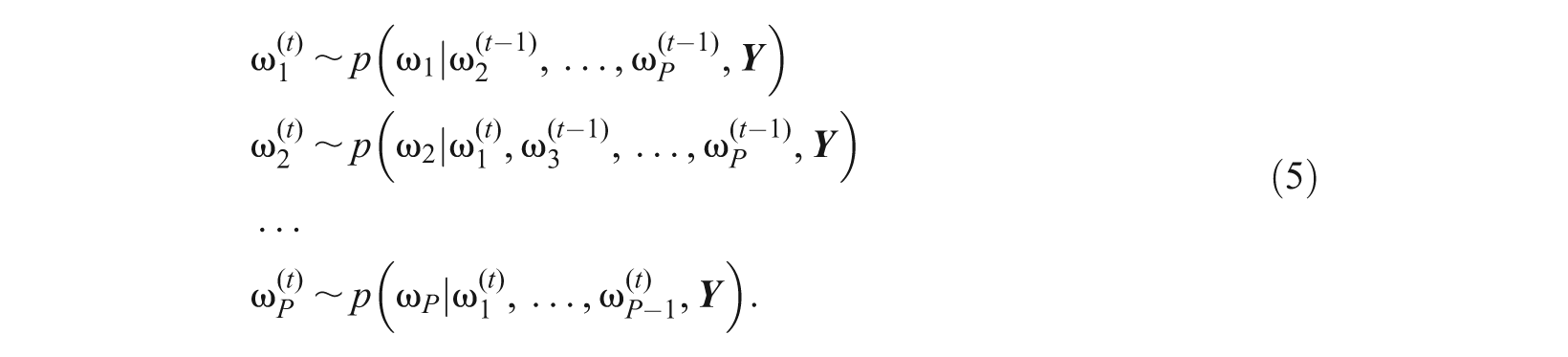The algorithm starts with initial values $ω^{(0)} = (ω_{1}^{(0)}, \dots, ω_{P}^{(0)})$ , and then iteratively updates ω^{(t − 1)} to ω^(t) by sampling as follows:

\begin{array}{l} ω_{1}^{(t)} ~ p (ω_{1} | ω_{2}^{(t - 1)}, …, ω_{P}^{(t - 1)}, Y) \\ ω_{2}^{(t)} ~ p (ω_{2} | ω_{1}^{(t)}, ω_{3}^{(t - 1)}, …, ω_{P}^{(t - 1)}, Y) \\ \dots \\ ω_{P}^{(t)} ~ p (ω_{P} | ω_{1}^{(t)}, …, ω_{P - 1}^{(t)}, Y) . \end{array}

The distribution of ω^(t) converges to the posterior distribution p(ω| Y ), regardless of the particular initial values. Therefore, the initial values do not affect the parameter estimates, given a sufficiently long chain. In practice, the first B iterations in a chain (ω⁽⁰⁾, …, ω^(T) of length T are discarded to help reduce the influence of the initial values (“burn-in”). The posterior mean of the marginal posterior distribution p(ω| Y ) of a parameter ω is a point estimate $\hat{ω}$ for the parameter (EAP estimate), which can be approximated by the mean of the samples:

\hat{ω} = \frac{1}{(T - B)} \sum_{t = B + 1}^{T} ω^{(t)} .

Albert (1992) used Gibbs sampling to estimate normal-ogive two-parameter models. Patz and Junker (1999a, 1999b) presented (closely related) Metropolis-within-Gibbs algorithms to estimate two-parameter logistic (2PL) and generalized partial credit model parameters.

Several studies have compared the performance of MML and MCMC estimation in dichotomous models (e.g., Albert, 1992; Baker, 1998; S.-H. Kim, 2001; S.-H. Kim & Cohen, 1999). Comparing an implementation of Albert’s (1992) Gibbs sampling scheme with BILOG, Baker (1998) concluded that the estimates were similar except in case of shorter tests and smaller samples where the BILOG estimates were superior. BILOG was also better at estimating item discrimination parameters. S.-H. Kim and Cohen (1999) compared the performance of marginalized Bayesian and Gibbs sampling for the 2PL model and found that marginalized Bayesian sampling performed better than the Gibbs sampler. It must be noted that S.-H. Kim and Cohen (1999) used very vague priors for the difficulty parameter (SD of 10,000), which may have affected the parameter estimates. S.-H. Kim (2001) compared the estimates from MML (and other methods) and Gibbs sampling for the Rasch model, and found no difference between the item parameter estimates, apart from the longer estimation time for MCMC. Because the true parameters were not known in this study, it is difficult to conclude which method was better at estimating person ability parameters.

S.-H. Kim and Cohen (1999), Kim (2001), and S.-H. Baker and S.-H. Kim (2004) suggested that Gibbs sampling and MCMC techniques may perform better with more complex models, for instance, polytomous item response models. Wollack, Bolt, Cohen, and Lee (2002) compared MML and MCMC parameter estimation for the nominal response model. They found that the two methods are similarly accurate in samples of 300 and 500 persons with test lengths of 10, 20, and 30 items. De la Torre, Stark, and Chernyshenko (2006) concluded that MML and MCMC parameter estimates in the generalized graded unfolding model (GGUM) were comparable; standard errors were more accurately recovered by MCMC. Roberts and Thompson (2011) found that MCMC had an advantage over MML for GGUM items with less than four response categories.

Purpose of the Present Study

The purpose of the present study was to compare the accuracy of MML and MCMC in recovering item and person parameters in Samejima’s (1969) graded response model (GRM) under varying conditions of latent trait distribution, test length, and sample size. In particular, the present study considered the recovery of item and person parameters with smaller test lengths and sample sizes where Bayesian estimation may be advantageous. This is particularly important because GRMs are commonly used in measurement of attitudes, where subscales with as few as five items administered to fewer than 300 respondents are not uncommon. Practitioners could benefit from recommendations regarding minimum sample size and test length required for adequate item and person parameter recovery in GRMs. The present study primarily investigated (a) the accuracy of MCMC in recovering item and person parameters compared with MML, (b) the factors which contribute the most to accurate parameter recovery, and (c) the minimal conditions required for adequate parameter recovery.

The secondary purpose was to test the effectiveness of OpenBUGS (Lunn, Spiegelhalter, Thomas, & Best, 2009), a general purpose Gibbs sampling software that allows practitioners to use MCMC estimation without (extensive) programming. J.-S. Kim and Bolt (2007) presented an introduction to fitting item response models using OpenBUGS. Curtis (2010) provided OpenBUGS codes for common item response models and described how these codes can be adapted for more complex models, in particular longitudinal designs. OpenBUGS provides a flexible way to fit a wide variety of item response models, in contrast to software such as MULTILOG (Thissen, Chen, & Bock, 2003), which can only be used for a fixed set of models. However, before practitioners can confidently use OpenBUGS for more complex models, they need to know its accuracy in parameter recovery and the factors that influence the recovery the most.

Previous Studies on MML Estimation of GRMs

Whereas the nominal response model (NRM) can be used to analyze unordered categorical responses, Samejima’s (1969) GRM is used for ordered categorical data, for example, Likert-type scales. An item i with K categories is modeled by a discrimination parameter a_i and K − 1 threshold parameters b_i1, …, b_{i(K − 1)}. The probability that person n with latent trait parameter θ_n will select category 1 ≤k≤K in response to item i is given by

P (Y_{n i} = k | θ_{n}, a_{i}, b_{i 1}, …, b_{i K}) = P (θ_{n}, a_{i}, b_{i (k - 1)}) - P (θ_{n}, a_{i}, b_{i k}),

where b_i0 = − ∞, b_iK = ∞, and with b_i equal to b_{i(K − 1)} or b_ik,

P (θ_{n}, a_{i}, b_{i}) = \frac{exp (a_{i} (θ_{n} - b_{i}))}{1 + exp (a_{i} (θ_{n} - b_{i}))} .

Reise and Yu (1990), Ankenmann and Stone (1992), DeMars (2003), and Lautenschlager, Meade, and Kim (2006) investigated the accuracy of MML parameter recovery for the GRM for various latent trait distributions, test lengths, and sample sizes.

Reise and Yu (1990) studied parameter recovery for three different types of tests based on their item discrimination parameter values. Based on factor loadings, they selected a poor test with discrimination parameters between 0.44 and 0.75, an average test with discrimination parameters between 0.58 and 0.98, and a good test with discrimination parameters between 0.75 and 1.33. Each test had a fixed length of 25 items with five response categories each. For the most discriminating test, the average root mean square errors (RMSEs) were 0.08, 0.16, and 0.35 for item discrimination, item difficulty, and person parameters, respectively. Recovery was better at larger sample sizes (500 or more vs. 250) and slightly better for samples in which the latent trait was uniformly distributed rather than normally distributed or skewed.

Ankenmann and Stone (1992) extended the study of Reise and Yu (1990) by including test length as a design factor. Longer tests improved person parameter estimation with average RMSEs of approximately 0.5, 0.4, and 0.3 for 5, 10, and 20 items, respectively. Test length did not affect item parameter estimation. Lautenschlager et al. (2006) reported similar results. DeMars (2003) examined (among other issues) MULTILOG’s and PARSCALE’s recovery of GRM parameters. For sample sizes of 250 and 500, she reported average RMSEs for item discrimination as 0.14 and 0.10 and for category threshold parameters as 0.26 and 0.17. In addition, DeMars analyzed the variance in the logarithm of the absolute difference between generating parameters and parameter estimates accounted for by software package, latent trait distribution, and sample size. The latter accounted for 3% of the variance with other factors accounting for less than 1%. In all studies, the second and third thresholds, b₂ and b₃, were recovered slightly better than the first and last thresholds, b₁ and b₄. Sample size had an impact on item parameter recovery but little effect on person parameter estimates. This can be explained by the fact that in the MML framework, parameters are estimated for each examinee separately after item calibration. However, in a fully Bayesian framework, person parameters are estimated jointly with item parameters, and therefore, sample size could possibly affect person parameter estimation in MCMC.

Reise and Yu (1990) and Ankenmann and Stone (1992) recommended a minimum sample size of 500 to accurately estimate GRM parameters and samples as large as 1,000 or 2,000 in situations where structural parameter recovery is crucial; Lautenschlager et al. (2006) concurred, recommending against using fewer than five items and 300 respondents. Unfortunately, none of these studies presented a full analysis of variance to quantify the contribution of different factors toward the accuracy of GRM parameter estimation.

Method

The primary purpose of this study was to compare the performance of MML versus MCMC in parameter recovery. Therefore, the main factor in the study design was estimation method (MML, MCMC). Although the authors primarily compare MML/EAP with MCMC (EAP) person parameter estimates, they also included MML/MAP estimates. Based on previous studies, they varied latent trait distribution (normal, skew-normal, and uniform), test length (5, 10, 15, and 20 items), and sample size (75, 150, 300, 500, and 1,000 persons). The specific levels of the independent variables were selected to facilitate comparison with other studies. The independent variables were fully crossed resulting in 120 conditions (2 estimation methods×3 latent trait distributions×4 test lengths×5 sample sizes).

Data Simulation

For each of the 60 combinations of latent trait distribution, test length, and sample size, 100 data sets were generated. Person parameters were simulated from (a) a unit normal distribution N(0, 1), (b) a uniform distribution on the interval (−3, 3), and (c) a skew-normal distribution with skewness = 1.25 and kurtosis = 1.5. These different distributions allowed the investigation of the impact of a person parameter prior that may be “mismatched” with the population latent trait distribution. Random variates θ′ from the skew-normal distribution were generated by transforming unit normal variates θ according to Fleishman’s (1978) power transformation method; specifically, θ′ = a + bθ + cθ² + dθ³ with a = −0.282, b = 1.037, c = 0.282, and d = −0.042 (see Fan, Felsovalyi, Sivo, & Keenan, 2003). A new set of person parameters was simulated for each replication.

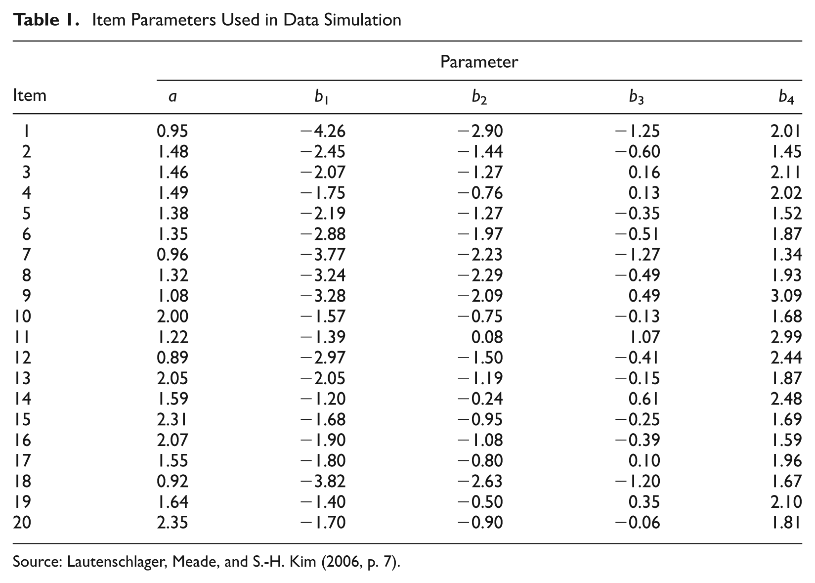
Common item parameters between replications help to minimize the effects of random error on parameter estimates. Therefore, response data were generated using item parameters for 20 items measured on a 5-point scale (see Table 1). These items have been calibrated from the Minnesota Satisfaction Questionnaire and were used by Lautenschlager et al. (2006). Using these item parameters ensured simulation of realistic items as advocated by Harwell, Stone, Hsu, and Kirisci (1996). A simulated test of length L contained the first L items.

Table 1.

Item Parameters Used in Data Simulation

	Parameter
Item	a	b ₁	b ₂	b ₃	b ₄
1	0.95	−4.26	−2.90	−1.25	2.01
2	1.48	−2.45	−1.44	−0.60	1.45
3	1.46	−2.07	−1.27	0.16	2.11
4	1.49	−1.75	−0.76	0.13	2.02
5	1.38	−2.19	−1.27	−0.35	1.52
6	1.35	−2.88	−1.97	−0.51	1.87
7	0.96	−3.77	−2.23	−1.27	1.34
8	1.32	−3.24	−2.29	−0.49	1.93
9	1.08	−3.28	−2.09	0.49	3.09
10	2.00	−1.57	−0.75	−0.13	1.68
11	1.22	−1.39	0.08	1.07	2.99
12	0.89	−2.97	−1.50	−0.41	2.44
13	2.05	−2.05	−1.19	−0.15	1.87
14	1.59	−1.20	−0.24	0.61	2.48
15	2.31	−1.68	−0.95	−0.25	1.69
16	2.07	−1.90	−1.08	−0.39	1.59
17	1.55	−1.80	−0.80	0.10	1.96
18	0.92	−3.82	−2.63	−1.20	1.67
19	1.64	−1.40	−0.50	0.35	2.10
20	2.35	−1.70	−0.90	−0.06	1.81

Source: Lautenschlager, Meade, and S.-H. Kim (2006, p. 7).

Parameter Estimation

MULTILOG was used to obtain MML item parameter estimates and MML/MAP person parameter estimates. The default starting values for item parameters were used (a = 1, b₁ = −1.39, b₂ = −0.405, b₃ = 0.405, and b₄ = 1.39). Based on the MML item parameter estimates, EAP person estimates (with unit normal prior) were computed using the authors’ Mathematica (Wolfram, 2011) code. MCMC model parameters were estimated using OpenBUGS. Following recommendations by Albert and Chib (1993) and Albert and Johnson (1999), a log-normal prior was used for the discrimination parameters, that is, $\log (a) ~ N (0, \sqrt{2})$ . Note that this implies µ(a) = 2.718 and σ(a) = 6.871. The authors chose a relatively noninformative uniform prior on the interval (−5, 5) for the threshold parameters, subject to the restriction b₁≤b₂≤b₃≤b₄. In other words, the only prior information on the difficulty parameters apart from the ordering was that their values were restricted to lie between −5 and 5. Person parameters were given a unit normal prior N(0, 1).

Initial values were provided for item parameters (a = 1, b₁ = −2, b₂ = −1, b₃ = 1, and b₄ = 2), whereas OpenBUGS generated initial values for person parameters. The first 1,000 iterations were allowed to burn in to reduce the effect of these initial values on the estimates. A further 10,000 iterations were used to estimate the parameters. To confirm the adequacy of this setup (which was also used by Wollack et al., 2002), the authors inspected one data set for each condition for nonconvergence. Specifically, two chains were run, and the multivariate potential scale reduction factor (Brooks & Gelman, 1998), estimated potential scale reduction (Gelman, 1996), and half-width test (Heidelberger & Welch, 1983) were computed using BOA (Smith, 2007). The 0.975th quantiles of both scale reduction factors were less than 1.2 for all conditions and all conditions passed the half-width test. This is commonly taken as an indication that the samples are drawn from the stationary distribution (see, for example, Smith, 2007). However, convergence assessment of Markov chains remains a difficult subject (see, for example, Sinharay, 2004). When analyzing a single data set, it may be prudent to allow more iterations to burn in.

MML and MCMC parameter estimates were equated to the metric of the generating parameters using the test characteristic curve method (Baker, 1992; Stocking & Lord, 1983) programmed by the authors. The accuracy of parameter recovery was then evaluated using RMSE, conditional bias, and correlations. With λ representing either discrimination a or one of the thresholds b₁, …, b₄, these were computed for each combination E×D×N×L×R (estimation method×distribution×sample size×test length×replication) as

RMSE (λ) = \sqrt{\frac{1}{L} \sum_{i = 1}^{L} {({\hat{λ}}_{R i} - λ_{i})}^{2}}

and

bias (λ_{i}) = \frac{1}{100} \sum_{R = 1}^{100} ({\hat{λ}}_{R i} - λ_{i}),

where ${\hat{λ}}_{Ri}$ is the estimate of parameter λi of item i in replication R. For each condition, RMSE of person parameters was computed as

RMSE (θ) = \sqrt{\frac{1}{N} \sum_{n = 1}^{N} {({\hat{θ}}_{R n} - θ_{R n})}^{2}},

where ${\hat{θ}}_{Rn}$ and θRn denote the estimated and generating value of the nth person parameter in replication R, respectively. Bias was computed for each person parameter as ${\hat{θ}}_{Rn} - θ_{Rn}$ , and binned averages of the conditional bias were plotted. Correlation between estimated and generating values was computed within each replication for each type of parameter (a, b₁, …, b₄, θ).

Fractional factorial analyses of variance of RMSEs and correlations were conducted by estimation method, latent trait distribution, sample size, and test length. Because the aim was to identify those conditions that contribute the most toward RMSE and correlations, the authors refrained from interpreting p-values and considered only η² effect sizes. They performed orthogonal planned contrasts to study differences in effect sizes between the levels of each factor. Because the authors deemed interaction effects between three or more factors difficult to interpret, only the four main effects and their six two-way interactions were considered.

Results

Tables 2 and 4 show the contribution of the design factors to the variance in RMSE and correlations of parameter estimates. Following Cohen (1988), effect sizes less than 1% were characterized as small, around 6% were characterized as medium, and greater than 14% were characterized as large were characterized. RMSE of item parameters was affected much more by sample size (η² > 35%) than by test length (η² < 1.65%). Similarly, RMSE of person parameters was affected by test length (η² = 86.30%) but not by sample size (η² = 0.32%). The interaction effect between sample size and test length was small for discrimination parameters (η² = 1.99%) and negligible for other parameters. Therefore, the authors present their results more succinctly by reporting RMSE averaged over test length for item parameters and over sample size for person parameters (see Tables 3 and 9). Test length had an effect on the correlation of discrimination, fourth threshold, and person parameters, so the authors report correlation by test length (see Tables 5 -7). In the following sections, they sequentially discuss item parameter recovery (including the impact of sample size ratio [SSR]), person parameter recovery, conditional bias, and computational time.

Table 2.

Effect Sizes (η²) of the Simulation Design Factors Explaining the Variabilities in RMSE of Parameter Estimates in Percentages

	Parameter
Source	a	b ₁	b ₂	b ₃	b ₄	θ
Estimation method (E)	0.02	2.23	0.78	0.13	0.22	0.04
Distribution (D)	2.55	4.96	2.19	0.28	4.29	2.62
Uniform versus normal, skewed	2.49	4.60	2.10	0.03	4.28	2.30
Normal versus skewed	0.06	0.36	0.09	0.25	0.01	0.32
Sample size (N)	47.09	43.83	35.46	68.17	56.48	0.32
75 versus 150, 300, 500, 1,000	37.01	32.48	25.87	46.71	40.25	0.28
150 versus 300, 500, 1,000	7.87	8.78	7.19	16.27	12.16	0.04
300 versus 500, 1,000	1.71	1.94	1.76	3.91	3.06	0.00
500 versus 1,000	0.51	0.63	0.65	1.28	1.01	0.00
Test length (L)	1.65	0.52	0.38	0.18	0.15	86.30
5 versus 10, 15, 20	1.62	0.07	0.01	0.14	0.10	66.54
10 versus 15, 20	0.03	0.39	0.36	0.03	0.00	17.00
15 versus 20	0.00	0.05	0.01	0.00	0.04	2.75
E×D	0.04	1.47	0.41	0.04	0.38	0.02
E×N	0.02	3.35	1.20	0.17	0.66	0.00
E×L	0.14	0.23	0.13	0.04	0.09	0.00
N×L	1.99	0.16	0.12	0.18	0.06	0.03
D×N	0.87	1.52	0.53	0.07	0.88	0.01
D×L	0.37	0.05	0.04	0.12	0.03	0.52
Total variance explained	54.72	58.31	41.23	69.38	63.24	89.86

Note: RMSE = root mean square error.

Table 3.

Mean RMSE in Item Parameter Estimates Under Different Conditions

		MML			MCMC			MML − MCMC
Sample size, N	Parameter	N	S	U	N	S	U	N	S	U
75	a	.417	.445	.299	.454	.476	.353	−.037	−.031	−.054
	b ₁	.860	.918	.490	.490	.530	.438	.370	.388	.052
	b ₂	.454	.491	.323	.326	.325	.297	.128	.166	.026
	b ₃	.238	.243	.239	.214	.223	.235	.024	.020	.004
	b ₄	.490	.489	.322	.405	.391	.351	.085	.098	−.029
150	a	.248	.266	.190	.261	.277	.201	−.013	−.011	−.011
	b ₁	.485	.558	.310	.377	.415	.321	.108	.143	−.011
	b ₂	.279	.302	.205	.241	.247	.210	.038	.055	−.005
	b ₃	.164	.169	.171	.156	.164	.171	.008	.005	.000
	b ₄	.314	.315	.223	.306	.296	.240	.008	.019	−.017
300	a	.171	.174	.132	.175	.177	.136	−.004	−.003	−.004
	b ₁	.326	.369	.213	.274	.305	.220	.052	.064	−.007
	b ₂	.199	.207	.145	.174	.176	.150	.025	.031	−.005
	b ₃	.114	.123	.120	.108	.119	.120	.006	.004	.000
	b ₄	.220	.219	.162	.218	.212	.169	.002	.007	−.007
500	a	.129	.134	.099	.132	.136	.101	−.003	−.002	−.002
	b ₁	.252	.270	.175	.213	.238	.174	.039	.032	.001
	b ₂	.153	.160	.115	.134	.143	.117	.019	.017	−.002
	b ₃	.090	.096	.092	.086	.095	.092	.004	.001	.000
	b ₄	.172	.170	.125	.170	.168	.129	.002	.002	−.004
1,000	a	.090	.096	.069	.092	.097	.070	−.002	−.001	−.001
	b ₁	.176	.194	.124	.155	.177	.121	.021	.017	.003
	b ₂	.103	.111	.083	.094	.102	.083	.009	.009	.000
	b ₃	.063	.073	.064	.060	.073	.065	.003	.000	−.001
	b ₄	.118	.125	.094	.117	.123	.096	.001	.002	−.002

Note: RMSE = root mean square error; MML = marginal maximum likelihood; MCMC = Markov chain Monte Carlo. RMSE averaged over items. Latent trait distribution: N = normal N(0, 1); S = skew-normal: skewness = 1.25, kurtosis = 1.5; U = uniform U(−3, 3). Absolute differences larger than .1 are boldfaced.

Table 4.

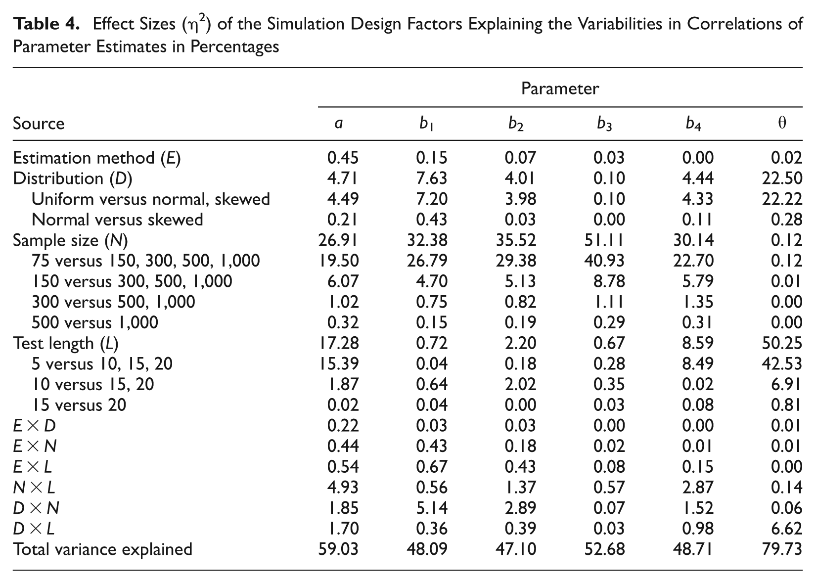
Effect Sizes (η²) of the Simulation Design Factors Explaining the Variabilities in Correlations of Parameter Estimates in Percentages

	Parameter
Source	a	b ₁	b ₂	b ₃	b ₄	θ
Estimation method (E)	0.45	0.15	0.07	0.03	0.00	0.02
Distribution (D)	4.71	7.63	4.01	0.10	4.44	22.50
Uniform versus normal, skewed	4.49	7.20	3.98	0.10	4.33	22.22
Normal versus skewed	0.21	0.43	0.03	0.00	0.11	0.28
Sample size (N)	26.91	32.38	35.52	51.11	30.14	0.12
75 versus 150, 300, 500, 1,000	19.50	26.79	29.38	40.93	22.70	0.12
150 versus 300, 500, 1,000	6.07	4.70	5.13	8.78	5.79	0.01
300 versus 500, 1,000	1.02	0.75	0.82	1.11	1.35	0.00
500 versus 1,000	0.32	0.15	0.19	0.29	0.31	0.00
Test length (L)	17.28	0.72	2.20	0.67	8.59	50.25
5 versus 10, 15, 20	15.39	0.04	0.18	0.28	8.49	42.53
10 versus 15, 20	1.87	0.64	2.02	0.35	0.02	6.91
15 versus 20	0.02	0.04	0.00	0.03	0.08	0.81
E×D	0.22	0.03	0.03	0.00	0.00	0.01
E×N	0.44	0.43	0.18	0.02	0.01	0.01
E×L	0.54	0.67	0.43	0.08	0.15	0.00
N×L	4.93	0.56	1.37	0.57	2.87	0.14
D×N	1.85	5.14	2.89	0.07	1.52	0.06
D×L	1.70	0.36	0.39	0.03	0.98	6.62
Total variance explained	59.03	48.09	47.10	52.68	48.71	79.73

Table 5.

Correlations Between Parameter Estimates and Generating Parameters by Estimation Method, Sample Size, and Test Length for Normal Latent Trait Distribution

		MML				MCMC
Sample size, N	Parameter	5	10	15	20	5	10	15	20
75	a	.459	.647	.793	.813	.208	.554	.766	.782
	b ₁	.802	.742	.767	.775	.736	.801	.863	.866
	b ₂	.896	.836	.894	.885	.852	.860	.925	.919
	b ₃	.941	.919	.943	.930	.932	.925	.947	.938
	b ₄	.535	.697	.736	.706	.496	.704	.782	.745
150	a	.604	.791	.880	.892	.438	.761	.875	.887
	b ₁	.932	.877	.894	.897	.881	.892	.917	.927
	b ₂	.958	.924	.945	.946	.933	.927	.955	.960
	b ₃	.974	.961	.965	.962	.968	.962	.967	.968
	b ₄	.694	.841	.855	.835	.612	.839	.875	.859
300	a	.783	.889	.939	.947	.712	.884	.939	.947
	b ₁	.967	.927	.943	.952	.948	.938	.954	.962
	b ₂	.982	.948	.972	.974	.975	.954	.976	.979
	b ₃	.987	.980	.984	.984	.987	.982	.985	.985
	b ₄	.824	.909	.916	.902	.796	.917	.922	.913
500	a	.836	.928	.962	.967	.812	.928	.962	.967
	b ₁	.983	.957	.968	.968	.980	.961	.970	.974
	b ₂	.989	.974	.985	.983	.988	.976	.985	.986
	b ₃	.991	.988	.990	.989	.991	.989	.990	.990
	b ₄	.882	.948	.950	.944	.882	.952	.950	.947
1,000	a	.910	.964	.981	.983	.904	.964	.981	.983
	b ₁	.991	.977	.983	.984	.991	.979	.985	.986
	b ₂	.996	.987	.992	.992	.996	.988	.992	.993
	b ₃	.996	.994	.995	.995	.996	.995	.996	.995
	b ₄	.940	.975	.973	.971	.941	.977	.973	.971

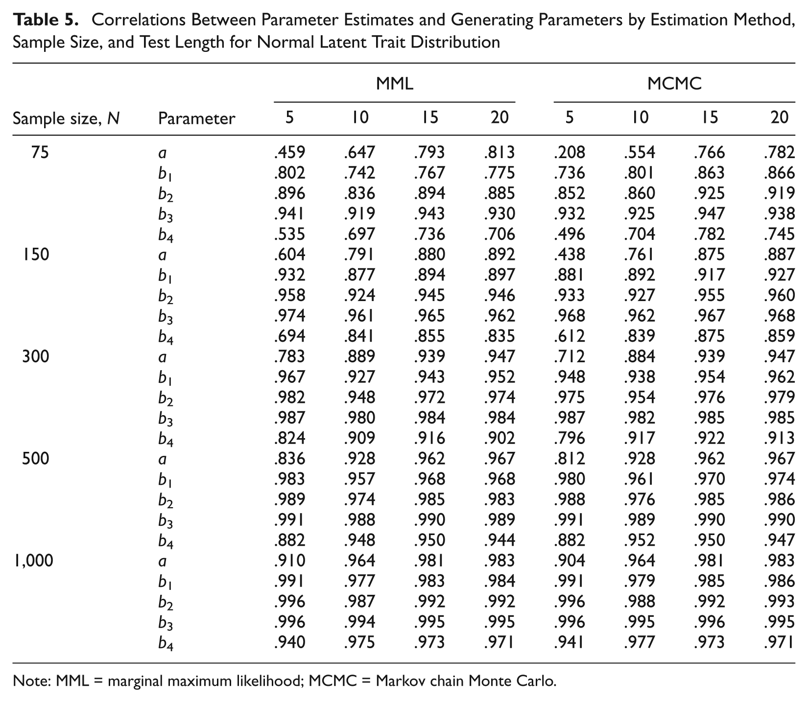
Note: MML = marginal maximum likelihood; MCMC = Markov chain Monte Carlo.

Table 6.

Correlations Between Parameter Estimates and Generating Parameters by Estimation Method, Sample Size, and Test Length for Skewed Latent Trait Distribution

		MML				MCMC
Sample size, N	Parameter	5	10	15	20	5	10	15	20
75	a	.458	.611	.769	.771	.202	.488	.731	.728
	b ₁	.756	.680	.743	.779	.696	.763	.835	.837
	b ₂	.882	.822	.882	.887	.856	.867	.921	.918
	b ₃	.947	.921	.937	.934	.939	.929	.944	.942
	b ₄	.449	.709	.736	.705	.405	.690	.770	.740
150	a	.608	.759	.841	.883	.419	.716	.827	.875
	b ₁	.916	.846	.870	.885	.836	.864	.896	.914
	b ₂	.965	.912	.940	.943	.935	.922	.950	.958
	b ₃	.973	.962	.967	.965	.966	.965	.971	.969
	b ₄	.709	.820	.837	.819	.643	.827	.858	.845
300	a	.738	.877	.924	.936	.636	.868	.922	.935
	b ₁	.951	.921	.930	.941	.921	.931	.942	.955
	b ₂	.978	.956	.972	.970	.967	.961	.976	.977
	b ₃	.986	.981	.983	.981	.986	.983	.985	.984
	b ₄	.775	.913	.905	.895	.740	.922	.914	.909
500	a	.803	.916	.948	.959	.760	.914	.949	.960
	b ₁	.973	.952	.957	.964	.964	.957	.962	.971
	b ₂	.986	.975	.980	.982	.982	.976	.982	.985
	b ₃	.992	.988	.989	.989	.991	.989	.990	.990
	b ₄	.843	.949	.943	.937	.832	.951	.946	.941
1,000	a	.893	.949	.975	.979	.880	.950	.975	.979
	b ₁	.986	.969	.980	.980	.983	.972	.981	.982
	b ₂	.993	.984	.991	.992	.992	.985	.992	.993
	b ₃	.995	.994	.995	.995	.996	.995	.995	.995
	b ₄	.917	.968	.972	.968	.919	.969	.972	.968

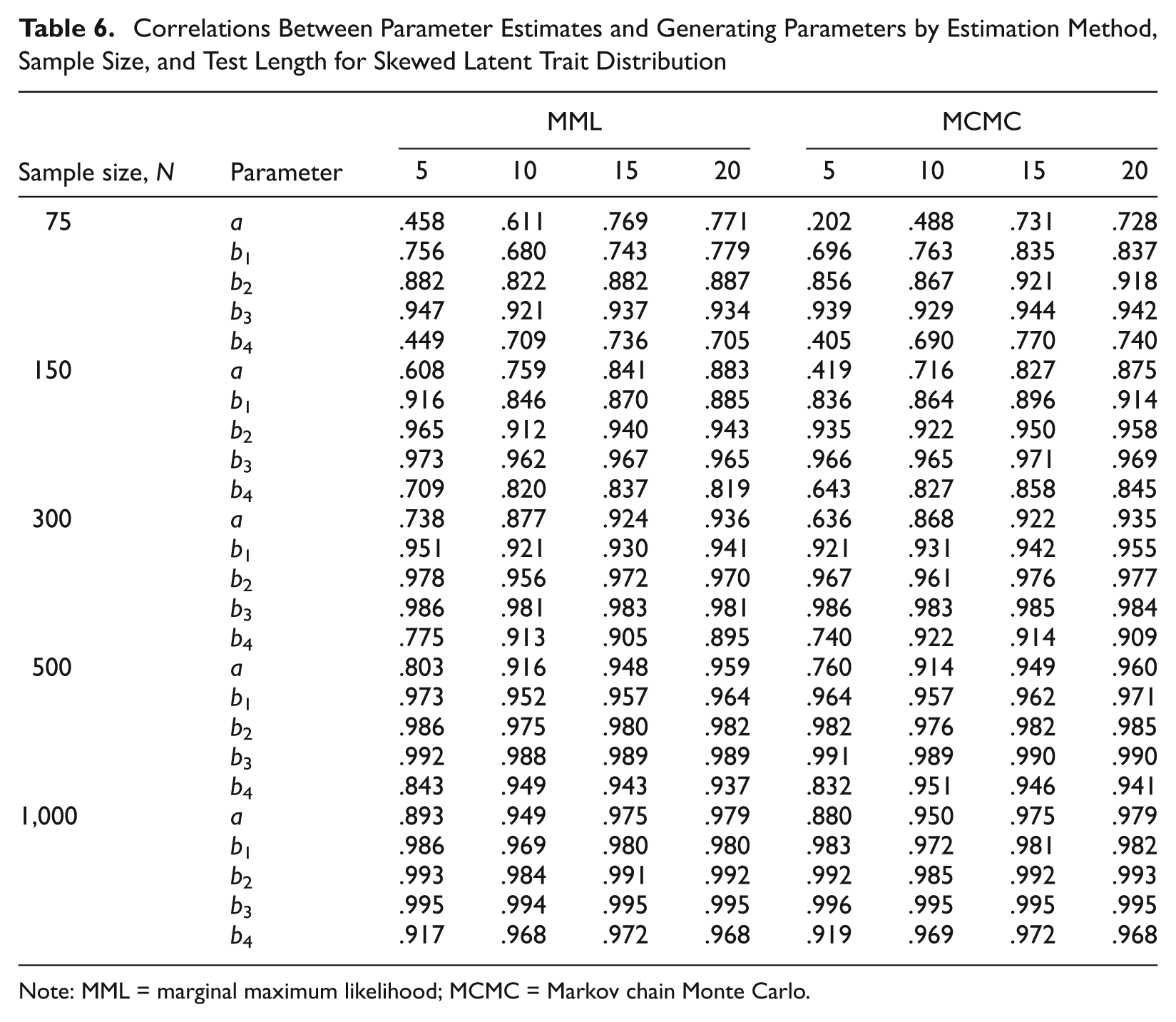
Note: MML = marginal maximum likelihood; MCMC = Markov chain Monte Carlo.

Table 7.

Correlations Between Parameter Estimates and Generating Parameters by Estimation Method, Sample Size, and Test Length for Uniform Latent Trait Distribution

		MML				MCMC
Sample size, N	Parameter	5	10	15	20	5	10	15	20
75	a	.665	.784	.867	.866	.633	.786	.869	.871
	b ₁	.957	.878	.910	.912	.959	.902	.926	.932
	b ₂	.964	.913	.944	.937	.965	.916	.945	.944
	b ₃	.939	.920	.931	.930	.941	.923	.933	.933
	b ₄	.704	.835	.863	.832	.689	.831	.860	.832
150	a	.789	.893	.932	.930	.787	.895	.933	.931
	b ₁	.980	.955	.960	.958	.981	.955	.959	.960
	b ₂	.980	.963	.972	.971	.981	.962	.971	.970
	b ₃	.967	.959	.966	.962	.968	.960	.966	.963
	b ₄	.858	.921	.925	.902	.850	.918	.920	.899
300	a	.856	.942	.960	.967	.856	.943	.960	.967
	b ₁	.990	.976	.980	.980	.991	.975	.979	.979
	b ₂	.991	.980	.986	.985	.991	.980	.985	.985
	b ₃	.984	.981	.983	.981	.984	.981	.983	.981
	b ₄	.902	.958	.959	.953	.897	.956	.957	.951
500	a	.908	.966	.977	.979	.907	.966	.978	.980
	b ₁	.994	.983	.987	.986	.994	.983	.987	.986
	b ₂	.994	.987	.991	.991	.994	.986	.991	.991
	b ₃	.992	.987	.989	.988	.992	.987	.989	.988
	b ₄	.945	.974	.977	.972	.943	.973	.976	.971
1,000	a	.959	.983	.988	.990	.959	.983	.988	.990
	b ₁	.998	.992	.993	.993	.998	.992	.993	.993
	b ₂	.997	.994	.995	.996	.997	.994	.995	.995
	b ₃	.995	.994	.995	.994	.995	.994	.995	.994
	b ₄	.970	.988	.987	.985	.969	.987	.987	.985

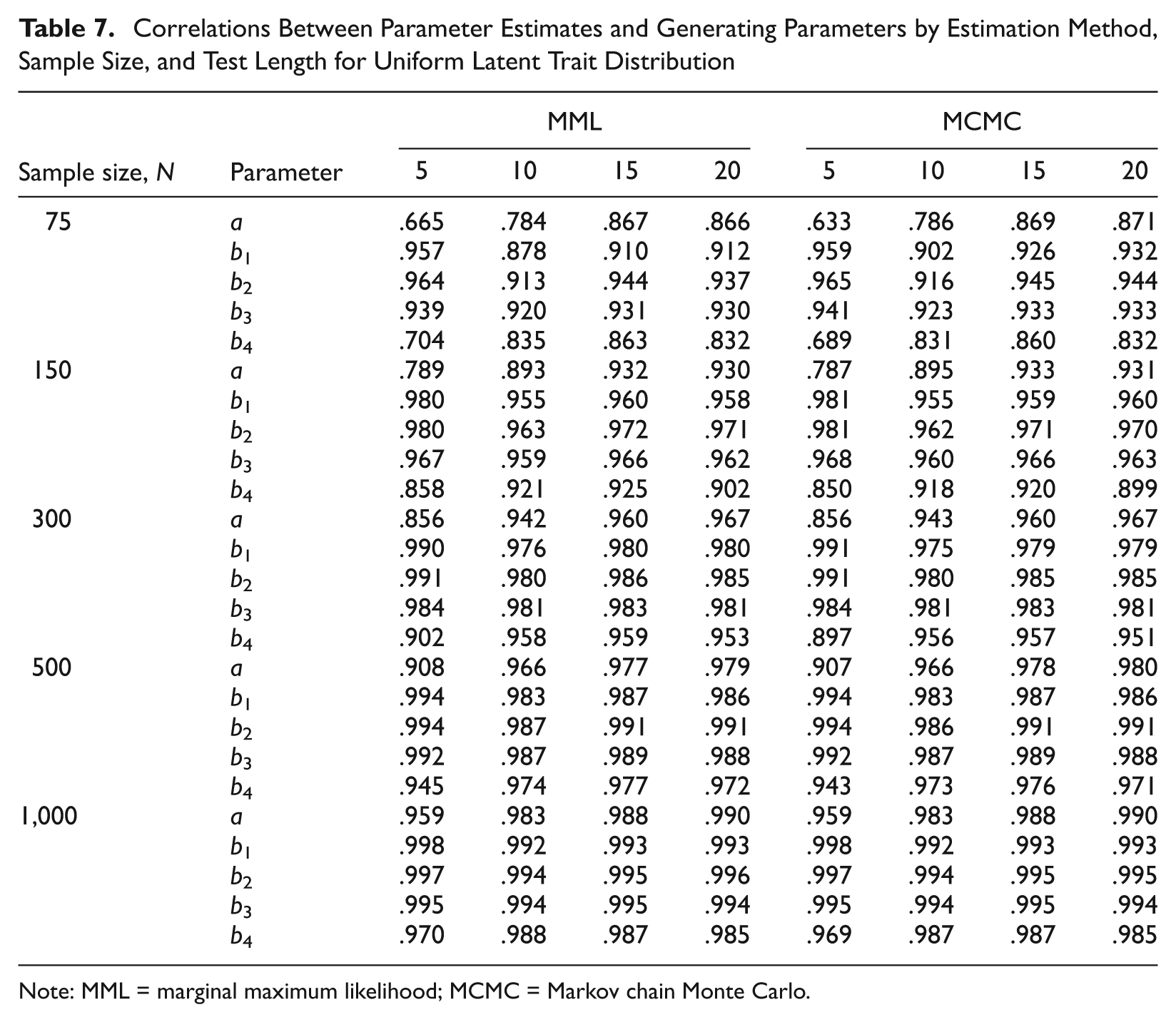
Note: MML = marginal maximum likelihood; MCMC = Markov chain Monte Carlo.

Table 8.

Mean RMSE in Item Parameter Estimates for Normal Distribution by SSR

		MML					MCMC
SSR	N:L	a	b ₁	b ₂	b ₃	b ₄	a	b ₁	b ₂	b ₃	b ₄
	75:5	.484	.795	.418	.220	.441	.735	.586	.376	.217	.461
	150:10	.242	.515	.294	.165	.321	.244	.386	.257	.158	.310
3:1	300:20	.157	.300	.183	.112	.228	.155	.234	.150	.104	.215
	250:5	.219	.356	.226	.148	.267	.146	.366	.209	.152	.256
	500:10	.124	.276	.170	.091	.179	.126	.239	.149	.087	.172
10:1	1000:20	.088	.162	.099	.062	.118	.089	.143	.088	.059	.115

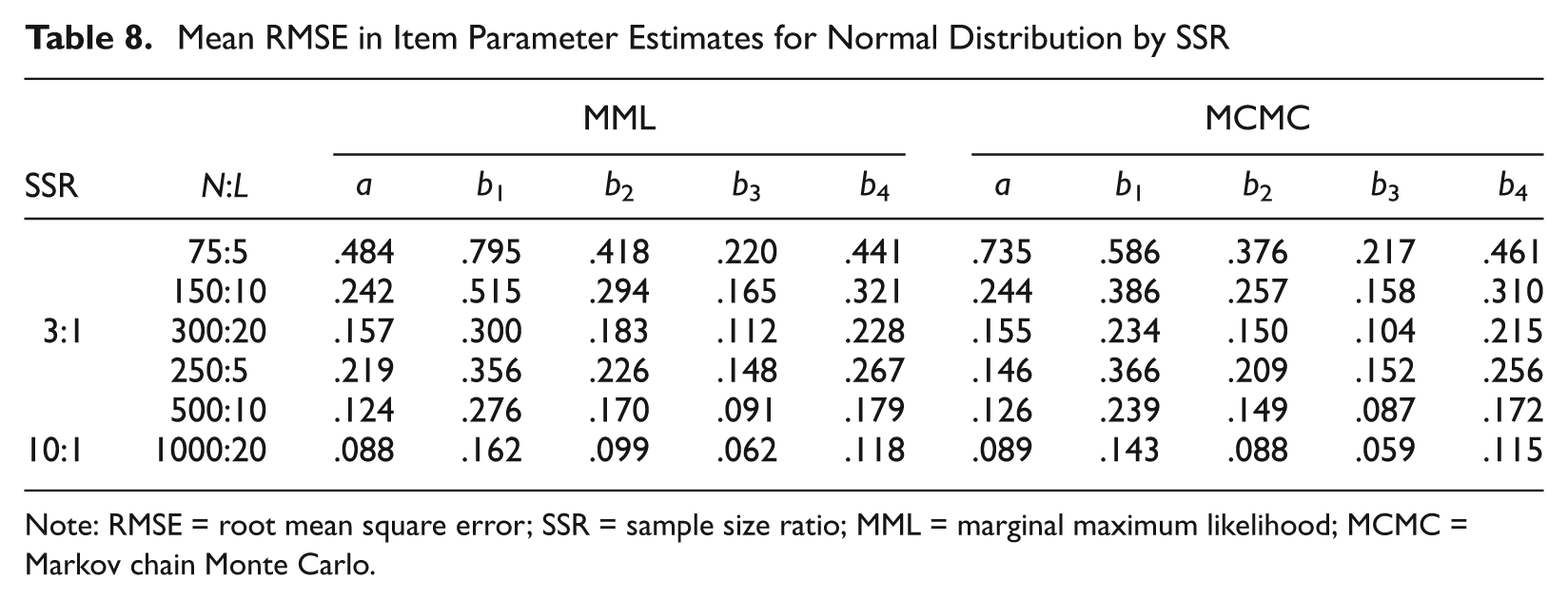
Note: RMSE = root mean square error; SSR = sample size ratio; MML = marginal maximum likelihood; MCMC = Markov chain Monte Carlo.

Table 9.

Mean RMSE in Person Parameter Estimates by Estimation Method, Latent Trait Distribution, and Test Length

	MML/EAP			MCMC			MML/MAP
L	N	S	U	N	S	U	N	S	U
5	.543	.564	.627	.552	.574	.622	.691	.720	.794
10	.413	.430	.459	.424	.442	.461	.664	.692	.721
15	.326	.339	.362	.336	.352	.371	.538	.572	.551
20	.274	.285	.304	.281	.293	.306	.475	.507	.513

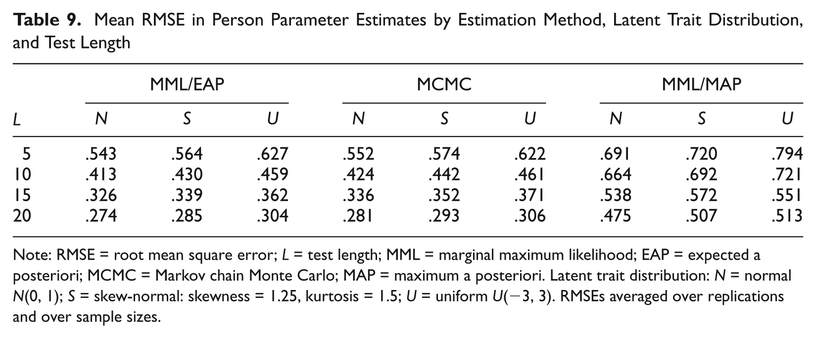
Note: RMSE = root mean square error; L = test length; MML = marginal maximum likelihood; EAP = expected a posteriori; MCMC = Markov chain Monte Carlo; MAP = maximum a posteriori. Latent trait distribution: N = normal N(0, 1); S = skew-normal: skewness = 1.25, kurtosis = 1.5; U = uniform U(−3, 3). RMSEs averaged over replications and over sample sizes.

Item Parameter Recovery

Sample size is the most important factor in item parameter recovery with effect sizes ranging from 35% to 68%. Orthogonal planned contrasts over various levels of sample size indicate that the maximum difference occurs between 75 versus (150, 300, 500, and 1,000), with a medium to large difference between 150 versus (300, 500, and 1,000). The gain in accuracy was smaller (η² < 3.91%) between samples of size 300 versus (500 and 1,000). Test length played a very small role in item parameter recovery.

Estimation method explained a small portion of the variation in RMSE for the first threshold parameter. MCMC recovered the first threshold better when N≤150, and additionally, the second threshold parameter when N = 75. For other conditions, RMSEs of the threshold parameters tend to be comparable between the two methods, with the first and last threshold parameters recovered less accurately than the middle two thresholds, probably because fewer respondents select these extreme categories (see Table 3). In general, MCMC did not recover discrimination parameters better than did MML. This echoes Baker’s (1998) study in which BILOG recovered discrimination parameters better than Gibbs sampling. Latent trait distribution explained a small percentage of the variation for discrimination parameters and threshold parameters, b₁, b₂, and b₄. Estimates from both methods were better for uniform latent trait distributions than normal and skew-normal. This is probably because a broader range of the latent trait in the sample provides more variation in responses. Note that for uniform distributions, MCMC did not recover item parameters any better than did MML.

Correlation is affected by latent trait distribution, sample size, and test length but not by estimation method (see Table 4). Correlations for item parameters (except the third threshold) are higher in uniformly distributed samples than in normally or skew-normally distributed samples (see Tables 5 -7). Sample size affects correlation primarily for samples of 75 and 150 persons. The effect of latent trait distribution and sample size on correlation can probably be explained by the fact that parameters are more accurately recovered in uniform and/or larger samples. Test length has a large effect on correlations of discrimination (η² = 17.28%) and fourth threshold (η² = 8.59%) parameters. Being an effect size, correlation should not be sensitive to the number of observations. Correlation may be affected by sample variance. For the generating item parameters, the SDs for a and b₄ increase with test length—for instance, SD(a) = 0.229, 0.309, 0.418, 0.454 for L = 5, 10, 15, 20—but the SDs of b₁, b₂, and b₃ remain relatively similar—for instance, SD(b₁) = 0.992, 0.889, 0.914, and 0.913 for L = 5, 10, 15, and 20, respectively. This could be a possible explanation for the test length explaining variation in the correlations of a and b₄.

SSR

De Ayala and Sava-Bolesta (1999) found that the recovery of item parameters in the nominal response model is affected more by SSR than by sample size alone. One might conjecture that this holds for the GRM as well. However, the impact of SSR over sample size is not apparent in Table 2. To investigate this issue further, RMSE for SSRs of 3:1 and 10:1 was compared with normal latent trait distribution but with different sample sizes. Because each item has five parameters in the present study, a SSR of 3:1 corresponds to conditions with sample size N to test length L ratios of 75:5, 150:10, and 300:20. Similarly, a SSR of 10:1 corresponds to N:L of 250:5, 500:10, and 1000:20. As N = 250, L = 5 was not among the authors’ original conditions, they additionally estimated 100 replications for this particular condition. Table 8 shows that even when SSR remains the same, item parameter estimates improve when the sample size increases. Doubling the sample size improves item parameter estimates by 159% on average.

Person Parameter Recovery

Test length explained the highest variance in RMSE of person parameter estimates (η² = 86.30%). The highest gain in accuracy was between test length of 5 versus 10, 15, and 20 (η² = 66.54%), followed by 10 versus 15 and 20 (η² = 17.00%); the gain between 15 items versus 20 items was much lower (η² = 2.75%). Correlation also improved with an increases in test length, probably because person parameters are estimated more accurately with longer tests. The distribution of the simulated person parameters explained a small amount of variance in RMSE (η² = 2.62%) but a large amount of variance in correlations (η² = 22.50%). RMSEs and correlations were a little higher in uniformly distributed versus normal and skewed samples, probably because the variability in parameter values is larger in that case.

Table 9 shows that RMSE in the MML/EAP and the MCMC person parameter estimates was comparable. However, the MML/MAP estimates were inferior to the other two estimation methods. RMSEs for MML/EAP and MCMC were approximately 50% to 70% lower than MML/MAP RMSEs. The MML/MAP estimates seem to be in line with the results of Reise and Yu (1990), who found an average RMSE in MAP person parameter estimates of 0.35 with a 25-item test of highly discriminating items. (Note that MML/EAP and MCMC produced better results even for tests with 5 fewer items.) Lautenschlager et al. (2006) also reported MML/MAP person estimates comparable with those obtained in the present study. DeMars (2003) reported an average RMSE of 0.67 using ML estimates from a 10-item test. In contrast, Ankenmann and Stone (1992) found substantially better RMSEs of approximately 0.5, 0.4, and 0.3, respectively, for 5-, 10-, and 20-item tests using MML/MAP.

The authors subsequently computed MML/MAP estimates using their own implementation of a MAP algorithm. The mean RMSEs for these MAP estimates were 0.53, 0.44, 0.37, and 0.38 for test lengths L = 5, 10, 15, and 20, respectively. These RMSEs are more comparable with the MML/EAP and MCMC results (but perhaps somewhat larger for L = 20). Moreover, Table 10 shows that there are essentially no differences in correlation between MML/MAP, MML/EAP, and MCMC person parameter estimates. Lautenschlager et al. (2006) also noted that person parameter estimates tend to correlate well with generating values, despite estimation errors that can be large with shorter test lengths.

Table 10.

Mean Correlation Between Person Parameter Estimates and Generating Parameters by Estimation Method, Latent Trait Distribution, and Test Length

	MML/EAP			MCMC			MML/MAP
L	N	S	U	N	S	U	N	S	U
5	.840	.825	.934	.837	.822	.934	.838	.822	.933
10	.911	.904	.965	.908	.901	.965	.905	.900	.960
15	.946	.941	.978	.943	.939	.978	.937	.933	.973
20	.962	.959	.985	.961	.958	.985	.953	.951	.980

Note: L = test length; MML = marginal maximum likelihood; EAP = expected a posteriori; MCMC = Markov chain Monte Carlo; MAP = maximum a posteriori. Latent trait distribution: N = normal N(0, 1); S = skew-normal: skewness = 1.25, kurtosis = 1.5; U = uniform U(−3, 3). Correlations averaged over replications and over sample sizes.

Conditional Bias

Bias in the ML estimates of GRM item parameters is known to be very small with samples larger than 300 persons (Lautenschlager et al. 2006; Reise & Yu, 1990). However, Bayesian estimates are regressed toward the mean of the prior distributions. This regression is stronger in smaller samples because, in these cases, the effect of the prior is larger relative to the likelihood. Moreover, more extreme values tend to regress more toward the mean.

Figures 1 and 2 show the conditional bias in item parameter estimates by sample size. In samples of 300 persons, maximum absolute bias in the item parameter estimates was 0.056, 0.296, 0.187, 0.080, and 0.115 for a, b₁, b₂, b₃, and b₄, respectively. This maximum absolute bias is roughly halved in samples of 500, except that there is no reduction in bias for b₄. Almost all discrimination parameters were overestimated. This may be due to the fact that the mean of the log-normal prior was larger than any of the generating discrimination values. In samples of 75 persons, the bias was particularly large compared with the bias in larger samples. The value of discrimination parameters seems to have no systematic effect on bias.

Figure 1.

Conditional bias in MCMC discrimination parameter estimates by sample size

Figure 2.

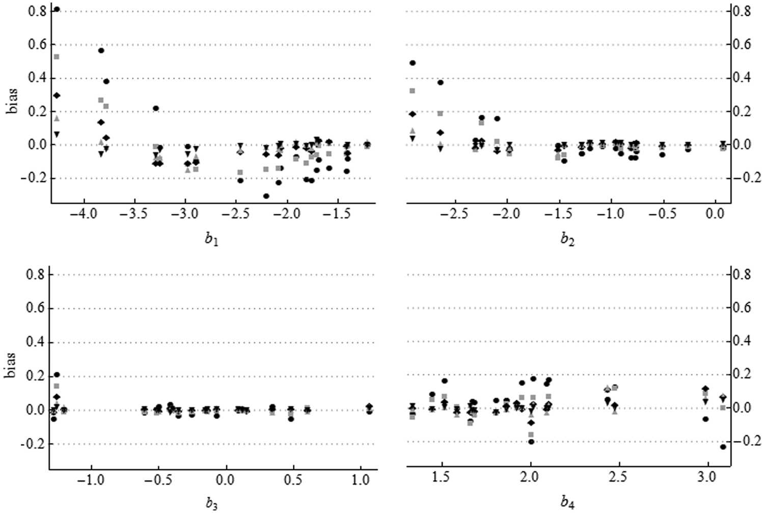
Conditional bias in MCMC threshold parameter estimates by sample size

However, the value of the threshold parameters has an effect on the bias in threshold parameters: The bias is lower in estimates of threshold parameters between −1.5 and 1.25. This is probably due to the fact that more responses are available to estimate these thresholds. In addition, the type of threshold parameter (first, second, etc.) also has an effect. For example, the first threshold of the sixth item b₆₁ and the second threshold of the first item b₁₂ are almost equal (about −2.9), but the biases in their estimates (when N = 300) are −0.109 and 0.187, respectively. The first thresholds are underestimated and the second thresholds are overestimated in the region where they overlap. This effect may be caused by the fact that the second threshold is forced to be above the first in the model specification.

Figure 3 shows bias in person parameters averaged over evenly spaced intervals of length 0.25 from −3 to 3 with least-square best-fitting cubic curves superimposed. The regression toward the mean is clearly visible. Bias in the MML/EAP estimates was slightly smaller than the bias in the MCMC estimates. Average absolute bias in the MML/EAP person estimates was 0.433, 0.330, 0.260, and 0.218 for test lengths L = 5, 10, 15, and 20, respectively, and 0.437, 0.333, 0.263, and 0.221 for MCMC person parameter estimates. Seong, S.-H. Kim, and Cohen (1997) found that EAP estimates were slightly less biased than MAP estimates for the GRM. Given that RMSE in MML/EAP estimates was considerably lower than in the MML/MAP estimates, the authors do not consider the bias in ML/MAP estimates further.

Figure 3.

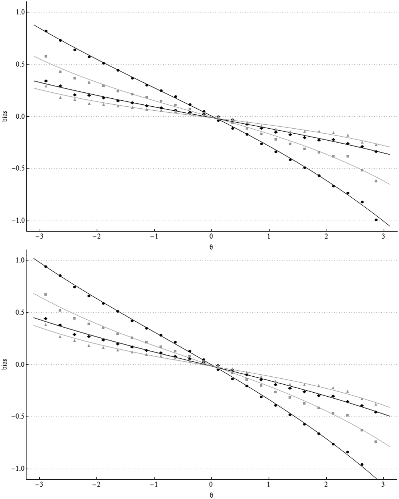
Conditional bias in MML/EAP (top) and MCMC (bottom) person parameter estimates by test length.

Estimation Time

Longer estimation time is a drawback of the MCMC estimation using OpenBugs (see Table 11). Modern hardware alleviates this problem to a certain extent. Wollack et al. (2002) reported that estimation of NRM parameters with 300 persons and 10 items took 4 hrs and 10 mins on a Pentium 450 MHz PC. This is considerably longer than the 7 min and 40 s it took on an Intel i3 3.2 GHz PC to estimate the GRM parameters for the same sample size and test length. Doubling the sample size increases the MCMC estimation time by a factor of 2.25 on average; doubling the test length multiplies estimation time by 2.17 on average. In comparison, the MML estimation with MULTILOG only takes a few seconds, even with larger samples.

Table 11.

Mean Estimation Time in Minutes for MCMC Estimation

	Sample size, N
Test length, L	75	150	300	500	1,000
5	0.70	1.54	3.58	6.45	15.90
10	1.40	3.07	7.67	15.45	34.88
15	2.11	4.80	12.83	25.12	53.72
20	2.81	6.54	19.27	34.73	72.87

Note: MCMC = Markov chain Monte Carlo. A total of 11,000 iterations in OpenBUGS on an Intel i3 3.2 GHz PC with 4 GB RAM.

Discussion

Several researchers have suggested that Bayesian (MCMC) parameter estimation may be more accurate than MML with smaller samples and test lengths, and with more complex models (S.-H. Kim, 2001; S.-H. Kim & Cohen, 1999; Swaminathan & Gifford, 1982). The present simulation study compared MML/EAP and MCMC parameter estimation in the GRM investigating (a) the accuracy of MCMC in recovering item and person parameters compared with MML/EAP, (b) the factors which contribute the most to accurate parameter recovery, and (c) the minimal conditions required for adequate parameter recovery.

Sample size is the most important factor in the accurate recovery of item parameters. Test length does not influence item parameter recovery. This concurs with results of Ankenmann and Stone (1992), among others. Improved item parameter recovery was associated with larger sample sizes, rather than higher SSRs, in contrast to findings by De Ayala and Sava-Bolesta (1999) for the nominal response model. The recovery of item parameters improved considerably when sample size increased from 150 to 300 examinees, to a lesser extent when sample size increased from 300 to 500 examinees, and even less when sample size increased from 500 to 1,000 examinees. It seems that 300 examinees are a necessary minimum; 500 persons are better. In practice, the limited increase in accuracy between samples of 500 and 1,000 persons may not be worth the additional costs. Practitioners may see considerably improved item parameter estimates if they select a sample with a broad range of latent traits. There is likely to be little negative effect of skewness in sampled latent traits.

Comparing the accuracy of MCMC with MML, there is little difference in item parameter recovery with samples of 300 persons or more, even in a polytomous item response model. This finding concurs with Wollack et al. (2002) and de la Torre et al. (2006) who also found no difference between samples of 300 persons and more for the nominal response model and the GGUM, respectively. The positive bias of MCMC in discrimination parameter estimates means that discrimination is likely to be overestimated, although this effect was small for large samples. The overestimation is probably caused by the choice of prior. Although a log-normal distribution seems a natural choice as prior for discrimination parameters, the mean of the prior was much larger than was the generating discrimination parameters. A prior better matched to the specific generating parameters used in this study probably would have improved the accuracy of the estimates. The authors are cautious about recommending another prior for discrimination parameters because a generic prior is needed when, in practice, the item parameters are unknown. This seems an important topic for further study.

Although the RMSEs are smaller for sample sizes of 500, the difference between samples of 300 versus 500 and 1,000 explained a low-medium amount of variance in the RMSE of the item parameters. Perhaps a more prudent selection of priors can make accurate recovery of the GRM item parameters feasible in samples of 300 persons. MCMC recovered the first and second threshold parameters better than did MML/EAP in samples of 75 persons, and the first threshold in samples of 150 persons. The authors note that the size of the RMSEs makes the use of IRT in such small samples debatable.

Person parameter recovery was influenced most by test length. When accurate estimation of person parameters is important, at least 10 items (preferably 15) should be used. Given a need for shorter instruments, 15 items seems to be a reasonable option as more items do not lead to much improvement. Overall, MML/EAP and MCMC person parameter estimates were much better than MULTILOG’s MML/MAP estimates, irrespective of test length. At the same time, there was essentially no difference in the correlations between parameter estimates and generating parameters. This seems to indicate that the larger RMSEs for the MML/MAP estimates produced by MULTILOG are due to scaling issues. However, all parameter estimates were put on the metric of the generating parameters using the same equating procedure, and the implementation of MML/MAP gave estimates comparable with MML/EAP and MCMC. Therefore, it seems more likely that the differences are caused by variations in the implementation of the MAP procedure.

MCMC and MML estimation differ in the choice of item priors (always flat for MML, more possibilities for MCMC). Bayesian parameter estimation is sometimes presumed to work better in smaller samples because priors provide additional information. However, the flat priors used in this study for the threshold parameters conveyed no information beyond the restriction to the range (−5, 5), and the prior (used following Albert & Chib, 1993, and Albert & Johnson, 1999) for the discrimination parameter was in fact ill matched to the actual parameter values.

Moreover, the unit normal person parameter worked well even when it did not match the uniform or skewed latent trait distribution in the sample. Further research is needed to see if item parameter estimates can be improved (especially discrimination parameters), for example, by using more informative or hierarchical priors.

Mislevy (1986) extended MML to marginalized maximum a posteriori (MMAP) by incorporating item priors within MML. MMAP and MCMC differ in the details of the marginalization of person parameters. In MMAP, person parameters are marginalized with respect to the prior distribution before item parameter estimation. In MCMC, parameters are estimated jointly and the marginalization is with respect to the posterior distribution of the person parameters. Recently, Roberts and Thompson (2011) compared MML, MMAP, and MCMC estimates for the GGUM. They found evidence that MMAP gives better estimates than does MCMC, noting that MMAP may offer one of the advantages of MCMC (use of item priors) without its disadvantage (computational burden). It may be worthwhile to investigate MMAP estimation of GRM parameters.

At the same time, the main benefit to MCMC estimation is more complete information about model parameters in the form of a sample from their posterior distributions. How the posterior draws given by MCMC estimation can be used to address psychometric issues such as model assessment, item and person fit, and equating is currently an active area of research (see, for example, Baldwin, 2011; Sinharay, Johnson, & Stern, 2006; Zhu & Stone, 2011). In conclusion, the present study shows that MCMC parameter recovery is comparable with MML in most cases with advantages to MCMC in smaller samples. Given the accuracy of estimates, the use of OpenBUGS to estimate GRM parameters seems viable. The software allows great flexibility in modeling, even without extensive programming skills, and could be useful for more complex models for which MML may not have been implemented.

Footnotes

Acknowledgements

The authors would like to thank the anonymous reviewers for their useful comments that helped them to improve this manuscript.

Declaration of Conflicting Interests

The author(s) declared no potential conflicts of interest with respect to the research, authorship, and/or publication of this article.

Funding

The author(s) received no financial support for the research, authorship, and/or publication of this article.

References

Albert

J. H.

(1992). Bayesian estimation of normal ogive item response curves using Gibbs sampling. Journal of Educational Statistics, 17, 251-269.

Albert

J. H.

Chib

(1993). Bayesian analysis of binary and polychotomous response data. Journal of the American Statistical Association, 88, 669-679.

Albert

J. H.

Johnson

V. E.

(1999). Ordinal data models. New York, NY: Springer.

Ankenmann

R. D.

Stone

C. A.

(1992, April). A Monte Carlo study of marginal maximum likelihood parameter estimates for the graded model. Paper presented at the annual meeting of the National Council on Measurement in Education, San Francisco, CA.

Baker

F. B.

(1992). Equating tests under the graded response model. Applied Psychological Measurement, 16, 87-96.

Baker

F. B.

(1998). An investigation of the item parameter recovery characteristics of a Gibbs sampling approach. Applied Psychological Measurement, 22, 153-169.

Baker

F. B.

Kim

S.-H.

(2004). Item response theory: Parameter estimation techniques (2nd ed.). New York, NY: Taylor & Francis.

Baldwin

(2011). A strategy for developing a common metric in item response theory when parameter posterior distributions are known. Journal of Educational Measurement, 48, 1-11.

Béguin

A. A.

Glas

C. A. W.

(2001). MCMC estimation of multidimensional IRT models. Psychometrika, 66, 541-562.

10.

Bock

R. D.

Aitkin

(1981). Marginal maximum likelihood estimation of item parameters: Application of an EM algorithm. Psychometrika, 46, 443-459.

11.

Bock

R. D.

Lieberman

(1970). Fitting a response model for n dichotomously scored items. Psychometrika, 35, 179-197.

12.

Bradlow

E. T.

Wainer

Wang

(1999). A Bayesian random effects model for testlets. Psychometrika, 64, 153-168.

13.

Brooks

Gelman

(1998). Some issues in monitoring convergence of iterative solutions. Journal of Computational and Graphical Statistics, 7, 434-455.

14.

Cohen

(1988). Statistical power analysis for the behavioral sciences (2nd ed.). Hillsdale, NJ: Erlbaum.

15.

Curtis

S. M.

(2010). BUGS code for item response theory. Journal of Statistical Software, 36, 1-34.

16.

De Ayala

R. J.

Sava-Bolesta

(1999). Item parameter recovery for the nominal response model. Applied Psychological Measurement, 23, 3-19.

17.

de la Torre

Stark

Chernyshenko

O. S.

(2006). Markov chain Monte Carlo estimation of item parameters for the generalized graded unfolding model. Applied Psychological Measurement, 30, 216-232.

18.

DeMars

C. E.

(2003, April). Recovery of graded response and partial credit parameters in MULTILOG and PARSCALE. Paper presented at the annual meeting of the American Educational Research Association, Chicago, IL.

19.

Fan

Felsovalyi

Sivo

S. A.

Keenan

S. C.

(2003). SAS for Monte Carlo studies: A guide for quantitative researchers. Cary, NC: SAS Institute.

20.

Fleishman

A. I.

(1978). A method for simulating non-normal distributions. Psychometrika, 43, 521-532.

21.

Fox

J.-P.

(2010). Bayesian item response modeling: Theory and applications. New York, NY: Springer.

22.

Fox

J.-P.

Glas

C. A. W.

(2001). Bayesian estimation of a multilevel IRT model using Gibbs sampling. Psychometrika, 66, 271-288.

23.

Gelfand

E. A.

Smith

A. F. M.

(1990). Sampling-based approaches to calculating marginal densities. Journal of the American Statistical Association, 85, 398-409.

24.

Gelman

(1996). Inference and monitoring convergence. In Gilks

W. R.

Richardson

Spiegelhalter

D. J.

(Eds.), Markov chain Monte Carlo in practice (pp. 131-144). London, England: Chapman & Hall.

25.

Geman

(1984). Stochastic relaxation, Gibbs distributions, and the Bayesian restoration of images. IEEE Transactions on Pattern Analysis and Machine Intelligence, 6, 721-741.

26.

Harwell

M. R.

Stone

C. A.

Hsu

T.-C.

Kirisci

(1996). Monte Carlo studies in item response theory. Applied Psychological Measurement, 20, 101-125.

27.

Hastings

W. K.

(1970). Monte Carlo sampling methods using Markov chains and their applications. Biometrika, 57, 97-109.

28.

Heidelberger

Welch

P. D.

(1983). Simulation run length control in the presence of an initial transient. Operations Research, 31, 1109-1144.

29.

Janssen

Tuerlinckx

Meulders

de Boeck

(2000). A hierarchical IRT model for criterion referenced measurement. Journal of Educational and Behavioral Statistics, 25, 285-306.

30.

Kim

J.-S.

Bolt

D. M.

(2007). Markov chain Monte Carlo estimation of item response models. Educational Measurement: Issues and Practice, 26, 38-51.

31.

Kim

S.-H.

(2001). An evaluation of a Markov chain Monte Carlo method for the Rasch model. Applied Psychological Measurement, 25, 163-176.

32.

Kim

S.-H.

Cohen

A. S.

(1999, April). Accuracy of parameter estimation in Gibbs sampling under the two-parameter logistic model. Paper presented at the annual meeting of the American Educational Research Association, Montreal, Quebec, Canada.

33.

Lautenschlager

G. J.

Meade

A. W.

Kim

S.-H.

(2006, April). Cautions regarding sample characteristics when using the graded response model. Paper presented at the annual conference of the Society for Industrial and Organizational Psychology, Dallas, TX.

34.

Lord

F. M.

(1986). Maximum likelihood and Bayesian parameter estimation in item response theory. Journal of Educational Measurement, 23, 157-162.

35.

Lunn

Spiegelhalter

Thomas

Best

(2009). The BUGS project: Evolution, critique, and future directions. Statistics in Medicine, 28, 3049-3067.

36.

Metropolis

Rosenbluth

A. W.

Rosenbluth

M. N.

Teller

A. H.

Teller

(1953). Equation of state calculations by fast computing machines. Journal of Chemical Physics, 21, 1087-1092.

37.

Metropolis

Ulam

(1949). The Monte Carlo method. Journal of the American Statistical Association, 44, 335-341.

38.

Mislevy

R. J.

(1986). Bayes modal estimation in item response models. Psychometrika, 51, 177-195.

39.

Patz

R. J.

Junker

B. W.

(1999a). Applications and extensions of MCMC in IRT: Multiple item types, missing data, and rated responses. Journal of Educational and Behavioral Statistics, 24, 342-366.

40.

Patz

R. J.

Junker

B. W.

(1999b). A straightforward approach to Markov chain Monte Carlo methods in item response models. Journal of Educational and Behavioral Statistics, 24, 146-178.

41.

Reise

S. P.

(1990). Parameter recovery in the graded response model using MULTILOG. Journal of Educational Measurement, 27, 133-144.

42.

Roberts

J. S.

Thompson

V. M.

(2011). Marginal maximum a posteriori item parameter estimation for the generalized graded unfolding model. Applied Psychological Measurement, 35, 259-279.

43.

Samejima

(1969). Estimation of latent ability using a response pattern of graded scores [Psychometrika Monograph Supplement No. 17]. Richmond, VA: Psychometric Society.

44.

Seong

T.-J.

Kim

S.-H.

Cohen

A. S.

(1997, March). A comparison of procedures for ability estimation under the graded response model. Paper presented at the annual meeting of the National Council on Measurement in Education, Chicago, IL.

45.

Sinharay

(2004). Experiences with Markov chain Monte Carlo convergence assessment in two psychometric examples. Journal of Educational and Behavioral Statistics, 29, 461-488.

46.

Sinharay

Johnson

M. S.

Stern

H. S.

(2006). Posterior predictive assessment of item response theory models. Applied Psychological Measurement, 30, 298-321.

47.

Smith

B. J.

(2007). BOA: An R package for MCMC output convergence assessment and posterior inference. Journal of Statistical Software, 21,1-37.

48.

Stocking

M. L.

Lord

F. M.

(1983). Developing a common metric in item response theory. Applied Psychological Measurement, 7, 201-210.

49.

Swaminathan

Gifford

(1982). Bayesian estimation in the Rasch model. Journal of Educational Statistics, 7, 175-191.

50.

Thissen

Chen

Bock

(2003). MULTILOG 7 [Computer software]. Lincolnwood, IL: Scientific Software International.

51.

Wolfram Research, Inc. (2011). Mathematica 8 [Computer software]. Champaign, IL: Wolfram Research, Inc.

52.

Wollack

J. A.

Bolt

D. M.

Cohen

A. S.

Lee

Y.-S.

(2002). Recovery of item parameters in the nominal response model: A comparison of marginal maximum likelihood estimation and Markov chain Monte Carlo estimation. Applied Psychological Measurement, 26, 339-352.

53.

Zhu

Stone

C. A.

(2011). Assessing fit of unidimensional graded response models using Bayesian methods. Journal of Educational Measurement, 48, 81-97.