
Abstract
Multiple imputation (MI) has become a highly useful technique for handling missing values in many settings. In this article, the authors compare the performance of a MI model based on empirical Bayes techniques to a direct maximum likelihood analysis approach that is known to be robust in the presence of missing observations. Specifically, they focus on handling of missing item scores in multilevel cross-classification item response data structures that may require more complex imputation techniques, and for situations where an imputation model can be more general than the analysis model. Through a simulation study and an empirical example, the authors show that MI is more effective in estimating missing item scores and produces unbiased parameter estimates of explanatory item response theory models formulated as cross-classified mixed models.
Statistical models of data from educational research and other disciplines often have to deal with complex multilevel structures. In this article, the authors focus on item response theory (IRT) modeling of data sets, where the same set of exercise items are answered by several persons, resulting in a cross-classification of response scores at Level 1 within persons and items both at Level 2 (Beretvas, 2011; Fox, 2010; Van den Noortgate, De Boeck, & Meulders, 2003), and where items and/or persons belong to larger groups. A typical example of such a data structure is an educational testing and measurement study, where persons are repeatedly measured on the same sample set of items, with individual persons clustered in classes, schools, or a university’s campus locations (Level 3). Such a structure is illustrated in Figure 1. The cross-classification is evident from the crossing of the lines connecting items to scores. Tabular illustrations of similar data structures are given, for instance, by Beretvas (2011) and Goldstein (2010). Although all Level 1 cells in the current example have an element within them, it is possible to have some empty cells in case of missing items scores by some persons. In such situations, caution must be taken when employing specific IRT models to avoid biased estimates.
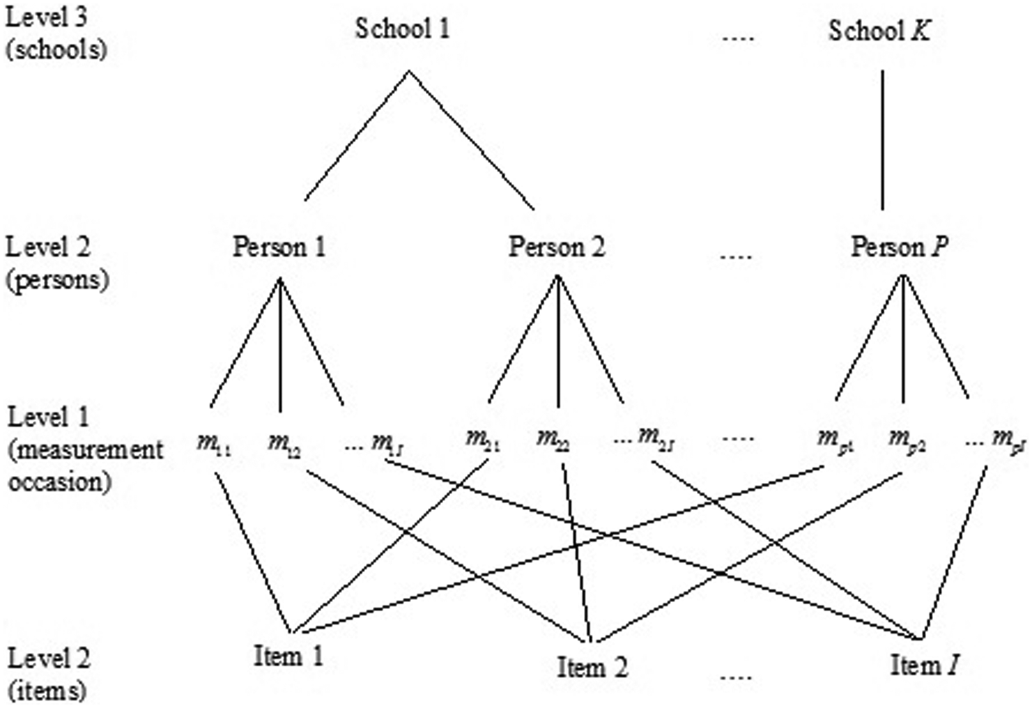
An illustration of a multilevel cross-classified data structure.
IRT Model With Crossed Random Effects
In IRT modeling, we can consider the measurement occasions (Level 1) to be nested within persons (Level 2), and treat person parameters as random effects, and characteristics of the measurement occasions (i.e., what item was solved at that moment) as predictors in an IRT model. A model with dummy item indicators as predictors is equivalent to the marginal maximum likelihood (ML) procedure for the Rasch model (De Boeck & Wilson, 2004; Rasch, 1993). Similarly items can be considered as being repeatedly measured such that measurement occasions are nested within items and person dummy variables can be included in the IRT model as predictors. However, items and persons can be regarded as random effects and fit cross-classification multilevel logistic models (Van den Noortgate et al., 2003) for binary multilevel IRT data. A fully unconditional (or an empty) two-level cross-classification IRT model which takes into account the variation between items, between persons, and within persons and items is given as
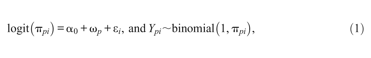
where
The cross-classified IRT model in Equation 1 can be recognized as a generalized linear mixed model (GLMM) that can be extended to an explanatory IRT framework by including person- and item-specific predictors (De Boeck & Wilson, 2004). Level 1 characteristics can also be included in the GLMM, say, the time or place at which a measurement of a person on an item was taken. The explanatory IRT framework is very flexible as it can be used to build different IRT models to explain latent properties of items, persons, groups of items, or groups of persons. For instance, if schools,

where
The model in Equation 2 includes several popular IRT models as special cases. For instance, the Linear Logistic Test Model (LLTM; Fischer, 1973) that is used to explain differences in item difficulty can be obtained, by dropping measurement predictors, person predictors and, the random item and school effects. De Boeck and Wilson (2004) showed that an interesting extension of the LLTM is an item explanatory IRT model that includes random item effects, referring to the part of the item difficulties that is not explained by the item predictors in the model. In the same way, differences in person ability can be explained by dropping measurement predictors, item predictors, and only including person predictors as fixed effects as in the case of a latent regression IRT model (Zwinderman, 1991) which De Boeck and Wilson call a person explanatory IRT model. By adding random person effects, the model does not assume that the person predictors explain all variance. For instance, Kamata (2001) has applied a latent regression model with person characteristic variables to analyze the effect of studying at home on science achievement. By dropping only the measurement predictors from Equation 2 and including person and item predictors, a doubly explanatory IRT model, in the terminology of De Boeck and Wilson, is obtained. Similarly, one can include only a Level 1 characteristic in the model or define several other IRT models from Equation 2. Moreover, Equation 2 can be extended to include meaningful group-by-item or person-by-measurement occasion random effects, though these are not considered further in the current study.
Presence of Missing Item Scores: Example of Electronic Learning Data
To build and improve their knowledge, persons can be taught in traditional classroom settings, via electronic learning (e-learning) environments, or through a combination of both. A specific kind of an e-learning environment is an item-based web environment in which persons learn by freely engaging exercise items online, receiving automatic feedback after each response, and in which their answers are centrally logged. The Maths Garden (Klinkenberg, Straatemeier, & Van der Maas, 2011) and the FraNel project (Desmet, Paulussen, & Wylin, 2006) are good examples of such e-learning environments. Such web-based e-learning environments might contain more items than a typical user makes, resulting in relatively large numbers of missing item scores (Wauters, Desmet, & Van den Noortgate, 2010). In such environments, the place or time at which measurements are taken can be influencing factors: whether a person is motivated to engage items at school, at home, or other public place; at start or completion of the course; toward a high-stakes or a low-stakes test; and so on. For instance, it is likely that an average student will tend to be more active in engaging the exercise items toward a graded examination period than at the beginning of the course. High amounts of missing item scores can be a major challenge when using IRT models to obtain reliable parameter estimates, usually giving rise to nonconvergence problems or intractable likelihoods (Fox, 2010).
Therefore, during statistical analysis of data with missing scores, variables and mechanisms that lead to missing items need to be identified and corrected for, to avoid biased estimates (Little & Rubin, 2002). In particular, using the terminology of Little and Rubin (2002), item scores can be missing completely at random (MCAR), missing at random (MAR), or missing not at random (MNAR). MCAR occurs when the probability of an item having a missing score does not depend on any of the observed or unobserved quantities (item responses or properties of persons or items). However, MCAR is a strong and unrealistic assumption in most studies because very often some degree of relationship exists between the missing values and some of the covariate data. It is often more reasonable to state that data are MAR, which occurs when a missing score depends only on some observed quantities that may include some outcomes and/or covariates. If neither MCAR nor MAR holds, then the missing scores that depend on the unobserved quantities and data are said to be MNAR. For instance, some students may not respond to certain items because they find them difficult.
These missing-data mechanisms need to be taken into account during statistical modeling to be able to produce estimates that are unbiased and efficient, although no modeling approach, whether for MCAR, MAR, or for MNAR, can fully compensate for the loss of information that occurs due to incompleteness of the data. In likelihood-based estimation, a missing score arising from MCAR or MAR is ignorable and parameters defining the measurement process are independent of the parameters defining the missing item process (Beunckens, Molenberghs, & Kenward, 2005). In case of a nonignorable missing item response arising from the MNAR mechanism, a model for the missing data must be jointly considered with the model for the observed data, which can for example be done using selection models and/or pattern-mixture models (cf. Molenberghs & Kenward, 2007). However, the causes of an MNAR mechanism might be unknown and the methods to implement its remediation are complex and beyond the scope of this study. Thus, MNAR is not further considered in the current study.
Handling of Missing Item Scores
Direct Likelihood (DL) Analysis
Modern statistical software for fitting cross-classification multilevel IRT models (e.g., SAS procedure GLIMMIX, SAS Institute Inc, 2005, and the lmer function of R package lme4, D. Bates & Maechler, 2010) are generally equipped with a full information ML analysis approach. An interesting feature of this approach, also known as DL analysis (Beunckens et al., 2005; Mallinckrodt, Clark, Carroll, & Molenberghs, 2003; Molenberghs & Kenward, 2007), is that it automatically handles missing responses under the assumption of MAR. Under the DL approach, all the available observed data are analyzed without deletion or imputation, using models that offer a framework from which to analyze clustered data by including both the fixed and random effects in the model, for example, GLMMs for non-Gaussian data. In doing so, appropriate adjustments valid under the ignorable missing mechanism are made to parameters, even when data are incomplete, due to the within-person correlation (Beunckens et al., 2005). An extensive description of the DL approach as a method for analyzing clustered data with missing observations is given in Molenberghs and Kenward (2007). In the next paragraph, a brief description of the approach is given in the context of the IRT model described in Equation 2.
The explanatory IRT models belong to the framework of GLMMs (De Boeck & Wilson, 2004) with persons as clusters and items for the repeated observations. The GLMM for observed binary item scores
Despite the attractiveness of the DL analysis, van Buuren (2011) advised that this approach should be used with some care when data are incomplete as it is only preferred to handle missing data if certain conditions hold. For instance, the standard DL analysis approach assumes that missing item scores are MAR. As such, the analysis model must include both the predictors of interest and all other covariates that may be related to the missingness process. But this can be suspect in some explanatory IRT models. For example, it can easily be deduced that the described person, item, and doubly explanatory IRT models are in fact distinct GLMMs—all nested in the general IRT model of Equation 2. Let us, for instance, revisit the e-learning environment example where students learn by freely engaging exercises online anywhere at anyplace. Suppose that items scores are missing as a result of differences in a Level 1 property (e.g., some persons may be motivated to engage exercise items in the afternoon than in the morning). Then fitting the item, the person, or the doubly explanatory IRT model may result in biased parameter estimates if the Level 1 property that is related to the missingness process is not included in the model, because this violates the MAR assumption. Yet, the requirement of including all covariates related to the missingness process has at least two challenges for the analyst. First, an analyst is forced to use a model that is not necessarily of interest. Second, the so-called complete model may be more complex to interpret (van Buuren, 2011) given the research objective of the analyst, or worse still, impossible to estimate given the available tools.
Imputation
A different approach to dealing with missing item scores in IRT data structures is by replacing the missing scores with simulated values—a process called imputation. Several imputation methods have been developed to deal with missing item scores in the IRT context. Most of these methods, like simple forms of mean imputation for the missing item scores, have been widely applied and examined in traditional IRT models (cf. Finch, 2008; Sheng & Carrière, 2005; van Ginkel, van der Ark, Sijtsma, & Vermunt, 2007). However, not very much has been done about missing responses in the area of multilevel IRT models with crossed random effects. Only recently, the performance of several imputation methods were compared in explanatory IRT models for multilevel educational data (Kadengye et al., 2012). The authors noted, however, that simple mean imputation approaches failed in clustered data structures and resulted in severely underestimated variability of the imputed data. This observation is in line with literature on missing data where simple forms of imputation are discouraged for multilevel data sets (cf. Little & Rubin, 2002; Schafer, 1997; van Buuren, 2011).
Imputation can take at least two different forms: single-value versus multiple-value. In single-value imputation, a missing score is replaced by one estimated value according to an imputation method of choice. However, Baraldi and Enders (2010) illustrated that several single-value imputation methods introduced bias in the estimates of means, variances, and correlations of a fictitious mathematics performance data set. The main problem is that inferences about parameters based on the filled-in single values do not account for imputation uncertainty, because variability induced by not knowing the missing values is ignored (Rubin & Schenker, 1986). As a result, the standard errors and confidence intervals of estimates based on imputed data can be underestimated and the Type I error rate of significance tests may be inflated (Baraldi & Enders, 2010; Little & Rubin, 2002; Schafer & Graham, 2002).
The multiple imputation (MI; Little & Rubin, 2002; Rubin, 1987) approach, however, involves replacing each missing item score by a set of more than one synthetic values generated according to an appropriate statistical model. However, some statistical programs that offer modules to implement MI for missing binary data, such as PROC MI (SAS Institute Inc, 2005) and R’s package MICE (van Buuren & Oudshoorn, 2000), generally ignore the clustering structure in multilevel data. Indeed, difficulties of some MI procedures to perform well in clustered data settings have been noted for various existing MI software (Yucel, 2008). To the best of knowledge, appropriate MI models for clustered data structures like those considered in the current study and the IRT models that are focused on—the cross-classified mixed models—have not been explored in the IRT literature. For an educational researcher with little statistical knowledge, it is not very clear as to which imputation model one can employ for such problems. This leaves such researchers at the mercy of existing MI software that are not appropriate for the data structures focused on, or perhaps to blindly employ DL analyses that may not be appropriate in some situations.
In this article, therefore, the authors compare the performance of an appropriate MI model based on empirical Bayes techniques versus a DL analysis for cross-classified multilevel IRT data. Generally speaking, an imputation model does not have to be similar to that of the final analysis, as the former can be allowed to contain structures or covariates that the latter model does not (Schafer, 2003; Yucel, 2008). More specifically, the focus is on situations where the variables that are of importance to understand missingness may not be of scientific interest to the analyst such that the MI model is more general than is any possible subsequent IRT analysis model. In the remainder of the article, the authors discuss the MI approach and an appropriate imputation model for missing item scores in cross-classified multilevel IRT data. Then through a simulation study, they compare results of a DL analysis and those obtained from multiply imputed data, in the situation where imputation and analysis models are similar, and where they are different. Next, they apply both approaches to an empirical example using different values for the number of imputations. The article concludes with a brief discussion.
MI Procedure
Plausible values for the missing item scores can be generated from the observed data by using MI procedures (Little & Rubin, 2002; Rubin, 1987). A model is used to generate
Different models can be adopted in the MI approach, but the exact choice typically depends on the nature of the variable to be imputed in the data set. For categorical variables, the log-linear model would be an appropriate imputation model (Schafer, 1997). However, the log-linear model can be applied only when the number of variables used in the imputation model is small (Vermunt, van Ginkel, van der Ark, & Sijtsma, 2008), making it feasible to set up and process a full multiway cross-tabulation as required for the log-linear analysis. Alternatively, imputations can be carried out under a fully conditional specification approach (van Buuren, 2007), where a sequence of regression models for the univariate conditional distributions of the variables with missing values is specified. Missing binary scores can be predicted with a logistic regression model of the observed scores on observed auxiliary variables with possible higher order interaction terms or on transformed variables. Such a logistic model can easily be implemented in MI modules like MICE (van Buuren & Oudshoorn, 2000) of R software.
However, a simple logistic regression model may not be suitable for estimating missing item scores in multilevel data sets. For instance, implementation of this model under MICE by Kadengye et al. (2012) resulted in biased estimates of the fixed and variance parameters for IRT models similar to the ones considered in the current study. To create good imputed data sets, it is desirable to reflect the data design in the model employed for creating the MIs (Rubin, 1987), as well as all other covariates available in the data set. Schafer (2003), however, cautions against making the imputation model unnecessarily large and complicated. For instance, he warns that in case some covariates are unrelated to the outcome variable but are included in the imputation procedure, precision of the analysis estimates may be reduced. Rather, a good imputation model should contain variables and structures that are correlated either with both the outcome and the missingness process or one of the two. For multilevel data, van Buuren (2011) described a MI Bayesian approach using a linear mixed-effects model such that the distribution of the parameters can be simulated by Markov chain Monte Carlo (MCMC) methods. However, full Bayesian and MCMC methods are beyond the scope of the current study. Instead, the authors confront the problem at hand by taking advantage of the asymptotic distributions of the parameters estimated from the IRT model fitted to the observed data.
Empirical Bayes Imputation Model
Let
with
Simulation Study
Through a simulation study, we studied the performance of the DL analysis and MI approach using the described imputation model for three explanatory IRT models: an item covariate model, a Level 1 covariate model, and a model with both covariates. The latter model is for a situation where the imputation and analysis models are similar. The models were fitted to data simulated under two situations, namely, a simple cross-classified IRT structure (Study I) and multilevel cross-classified IRT structure (Study II).
Simulating Data
Item response data were generated according to the model
Clustering
For Study I, a simple crossed-classified structure was considered where item difficulties were assumed to be generated from an item bank with a standard normal distribution,
Sample size
Two item sample sizes were compared, that is,
Distribution of covariates
In both simulation studies, the two covariates are assumed to be binary variables. The scores on these variables were drawn from a Bernoulli distribution with a probability parameter of .5 simply to obtain a generally balanced design.
Effect size of fixed effects
For both studies, a parameter value of
Missing proportions (
)
Each sample data set was used twice: a selection of 25% and then 50% of the item scores were removed, yielding moderate and high proportions of missing scores. These values were based on the authors’ experience with e-learning environments (because this is the example that is used) that tend to have high levels of nonresponse.
Missing mechanism
For all data samples, missingness at random (MAR) was induced in item scores. To induce the two missing proportions given the MAR process, probabilities of responding
Analysis Procedure
For both simulation studies, the authors assumed that an analyst may be interested in one of three explanatory IRT models: an item covariate model, a Level 1 covariate model, or a model that contains both covariates. If the Level 1 property is not included in the analysis model (for the item covariate IRT model), we expect increased bias in the fixed effects estimates for the DL analysis, because by excluding this covariate, the MAR process is violated as this covariate is associated with the missing item scores. For the other two models, we expect that the DL analysis and the MI approach to have more or less similar results and that bias will be minimized because the analysis model corrects for the underlying missing process. For the models where one of the predictors is dropped, the expected value for the intercept is equal to the average of the expected values for the two conditions distinguished based on the “population” parameter values of the intercept and the particular covariate not in the model. In this case, this value is
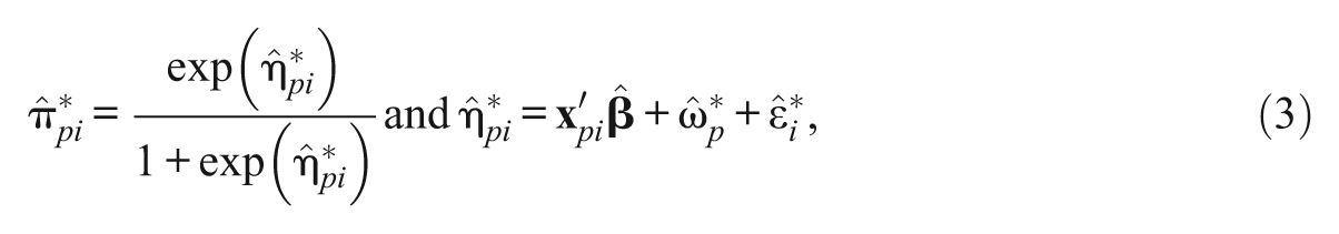
Imputations for the missing item scores were generated using the model for simulating the data. Under MI, the basic rule of thumb is that the number of imputations is usually set to
In the first study, analyses involved 4 conditions: 2 (item sample sizes) × 2 (missing proportions). In the second study, only two conditions: 1 (item sample size) × 2 (missing proportions) were considered because analyses of Study II are used for comparison purposes. In all, 500 data sets were simulated for each of the six conditions. Each data set was analyzed 9 times: the three models are fitted to the completely observed data, to the incomplete data, and to the data whose missing item scores have been multiply imputed according to Equation 3, resulting in 27,000 analyses. The purpose of analyzing the completely observed data sets (denoted CD) was to compare the performance of the MI procedures with the performance of the IRT analysis in the ideal situation, this is, when there is no missingness. Note that the number of conditions, and specifically the number of replications was kept relatively small due to estimation time considerations. For instance, the 500 replications of only one condition (e.g.,
Outcomes of interest are the accuracy of the fixed regression weights’ estimates, of the estimated standard errors of these fixed effects, and of the estimates for random effects’ variance over persons (
Model fitting was done in R statistical software version 2.12.1, as described by De Boeck et al. (2011). For each simulated data set, model parameters were estimated using the lmer() function in the package lme4 (D. Bates & Maechler, 2010). The Laplace approximation to the likelihood is optimized to obtain approximate values of the ML or restricted maximum likelihood (REML) estimates for the parameters of interest and for the corresponding conditional modes of the random effects (Doran, Bates, Bliese, & Dowling, 2007). In random effects models, the REML estimates of variance components are generally preferred because they are usually less biased than ML estimates (D. M. Bates, 2008; Sarkar, 2008). For the MI procedure, parameter estimation and the missing-data imputation were conducted alternatively. That is, in the DL analysis, a general GLMM in Equation 3 (for Study I) or the one with an additional random school effect (for Study II) was fitted to the observed data with incomplete scores. Obtained individual person and item random REML parameter estimates were then used to successively draw M = 10 plausible estimates from their asymptotic sampling distributions. These were then successively combined to the set of corresponding fixed linear predictor estimates, to obtain plausible probabilities of success for each person–item combination—the
Results
Fixed Effects’ Parameter Estimates
Estimated bias
Table 1 shows the bias and MSE of the fixed effects estimates by fitted model, missing proportion, analysis approach, and item sample size. For the item covariate model (Model 1, Table 1), the bias in estimates of the intercept parameter from the DL analyses is larger and not comparable with that of the CD analysis for all considered conditions. This bias increases when more item scores are missing. This is not the case when analyzing the multiply imputed data sets, where estimated bias in all parameters and across all conditions is generally comparable with that of the CD analysis. However and for the Level 1 covariate model across the two sample sizes (Model 2, Table 1), estimated bias from the DL analysis and MI approach is small and comparable with that obtained from the CD analysis, especially at 25% missing proportion. At 50% missing proportion, however, estimated bias in the intercept parameter for MI seems to be slightly larger than that of the DL analysis. Similar results are found for the analysis models that include both covariates (Model 3, Table 1). Because the covariate related to missing scores is included in the DL analysis, and as such the MAR mechanism is not violated, both the DL analysis and MI approach have comparable biases.
Bias and MSE in Fixed Effects’ Estimates by Fitted Model, Missing Proportion, Analysis Approach, and Study.
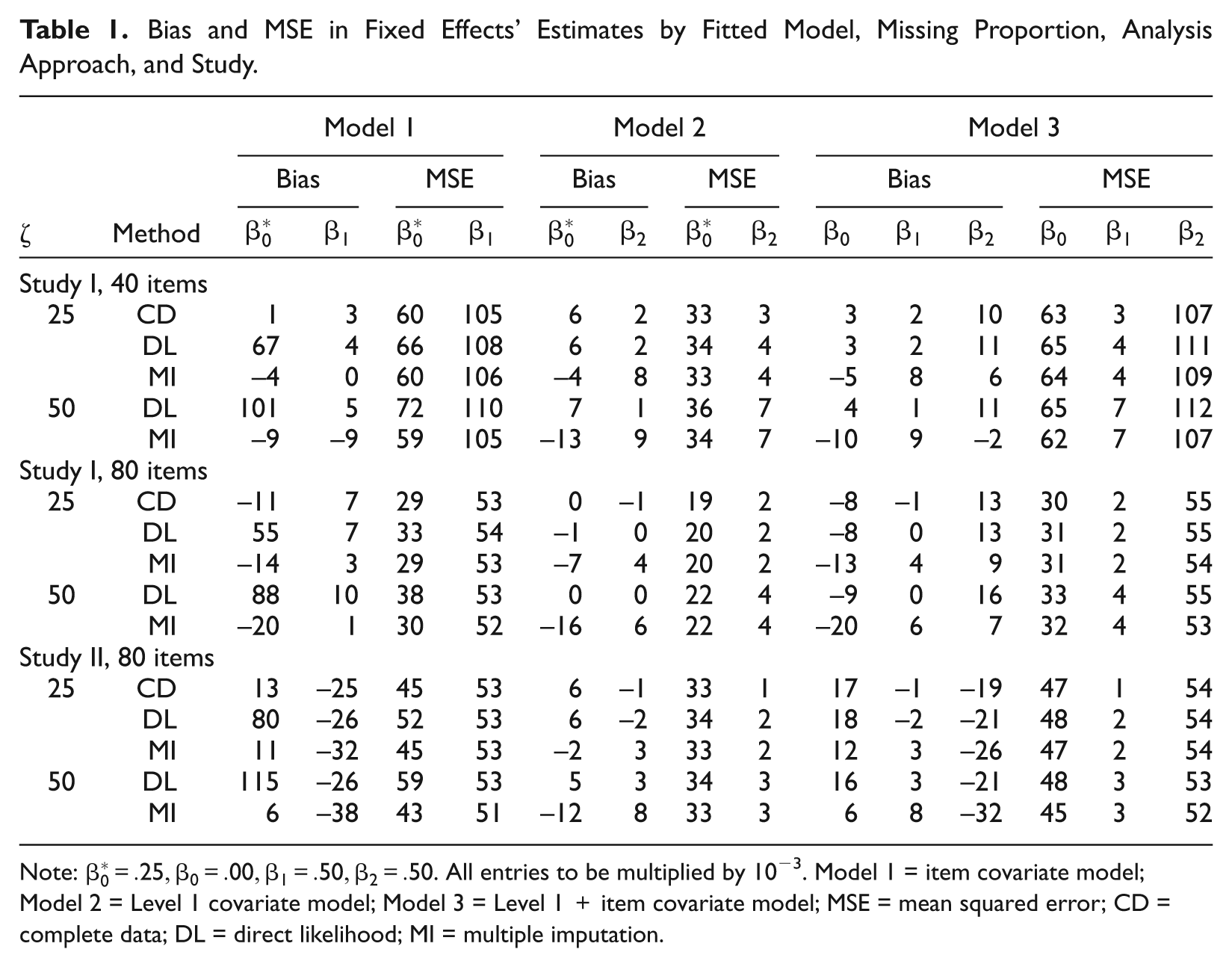
Note:
MSE
For the item covariate model (Model 1, Table 1), the MSE values for the intercept when using the DL approach are larger than those of the CD analysis for both missing proportions. However, the MSE values for all the parameter estimates of the item covariate model using the MI approach are comparable with those of the CD analysis for all the considered conditions. Indeed, for these estimates, the model used to impute missing item scores corrected for the covariate related to the missing scores—much as it was not of interest to the analyst. At 25% missing proportions, results for Models 2 and 3 (Table 1) indicate that the MSE in all parameter estimates for the DL and MI approaches are comparable with those given by the CD analysis. However, the MSE for the DL analysis tends to increase for the smaller item samples in which 50% of the scores are missing which is not the case for the MI approach.
Standard errors
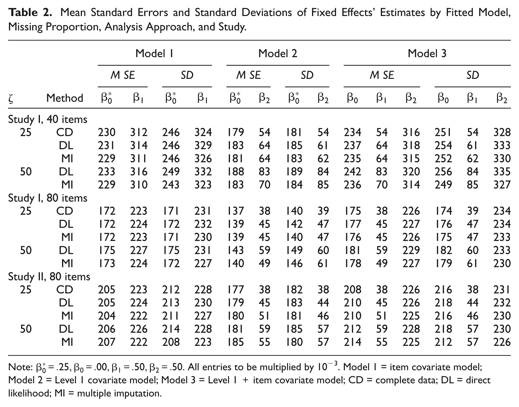
Table 2 shows the mean of the standard errors (mean SE) and standard deviations (SD) of the fixed effects estimates by fitted model, missing proportion, analysis approach, and item sample size. For all analysis approaches and in all conditions but especially for the smaller item samples, the SD of the estimates were slightly underapproximated by the estimated mean SE. At 50% missing proportions, the estimated mean SE and the respective SD of the estimates tend to get slightly larger both for the DL and MI approaches, but this is more pronounced in the DL approach. This is expected due to the increased uncertainty as a result of large amounts of missing scores and hence the decreased number of scores on which estimates are based. In general, for all models, there was little variation for both DL and MI approaches in the difference between the mean standard errors and their corresponding standard deviations.
Mean Standard Errors and Standard Deviations of Fixed Effects’ Estimates by Fitted Model, Missing Proportion, Analysis Approach, and Study.
Note:
Coverage percentages
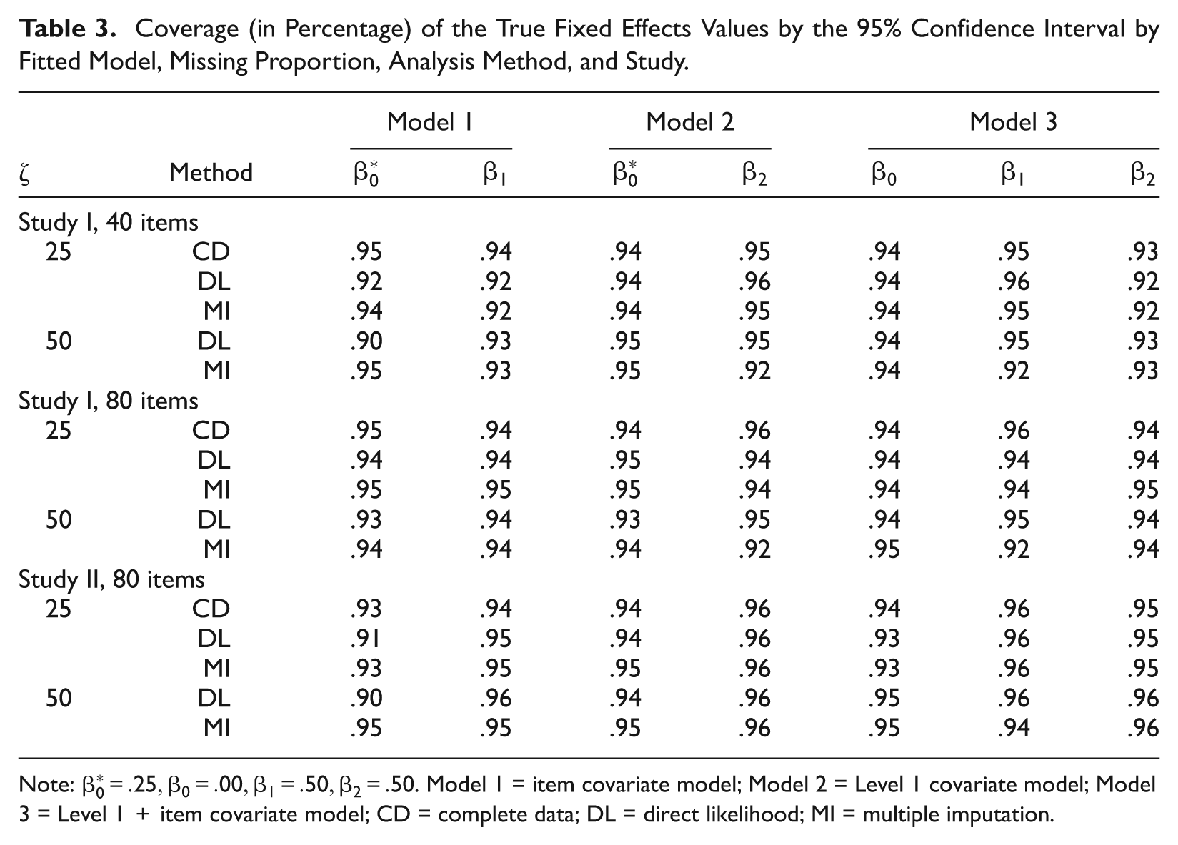
Coverage percentages of the true fixed effects values by the 95% confidence intervals are shown in Table 3. Good confidence intervals should have coverage probability equal (or close) to the nominal level of 95%. For the item covariate model (Model 1, Table 3), the coverage percentages for the intercept parameter when using the DL approach are generally smaller than the nominal value. This is not the case with the MI approach for this particular analysis model. In the other two analysis models (Models 2 and 3 of Table 3) and at 25% missing, the coverage percentages are comparable with those of the CD analysis. The MI approach tends to have coverage percentages slightly below the nominal value at 50% missing for the Level 1 covariate parameter estimate.
Coverage (in Percentage) of the True Fixed Effects Values by the 95% Confidence Interval by Fitted Model, Missing Proportion, Analysis Method, and Study.
Note:
Random Effects’ Variance Estimates
Estimated bias
Table 4 shows the bias and the MSE values of random effects’ variance estimates by fitted model, missing proportion, analysis approach, and item sample size. For all analysis models and for both DL and MI approaches, it can be seen that the bias of all random effects’ variance estimates increases when more data are missing. However, now, the bias seems to be slightly larger for the MI approach, but still in the same direction as that of the DL analysis. This is not unexpected because by replacing missing scores with imputed values sampled from the estimates of individual persons and items, the overall variability in the data set will decrease. This is probably also due to the shrinkage effect associated with empirical Bayes estimates from which imputations were drawn.
Bias and MSE in Random-Effect Variance Estimates by Fitted Model, Missing Proportion, and Analysis Approach.
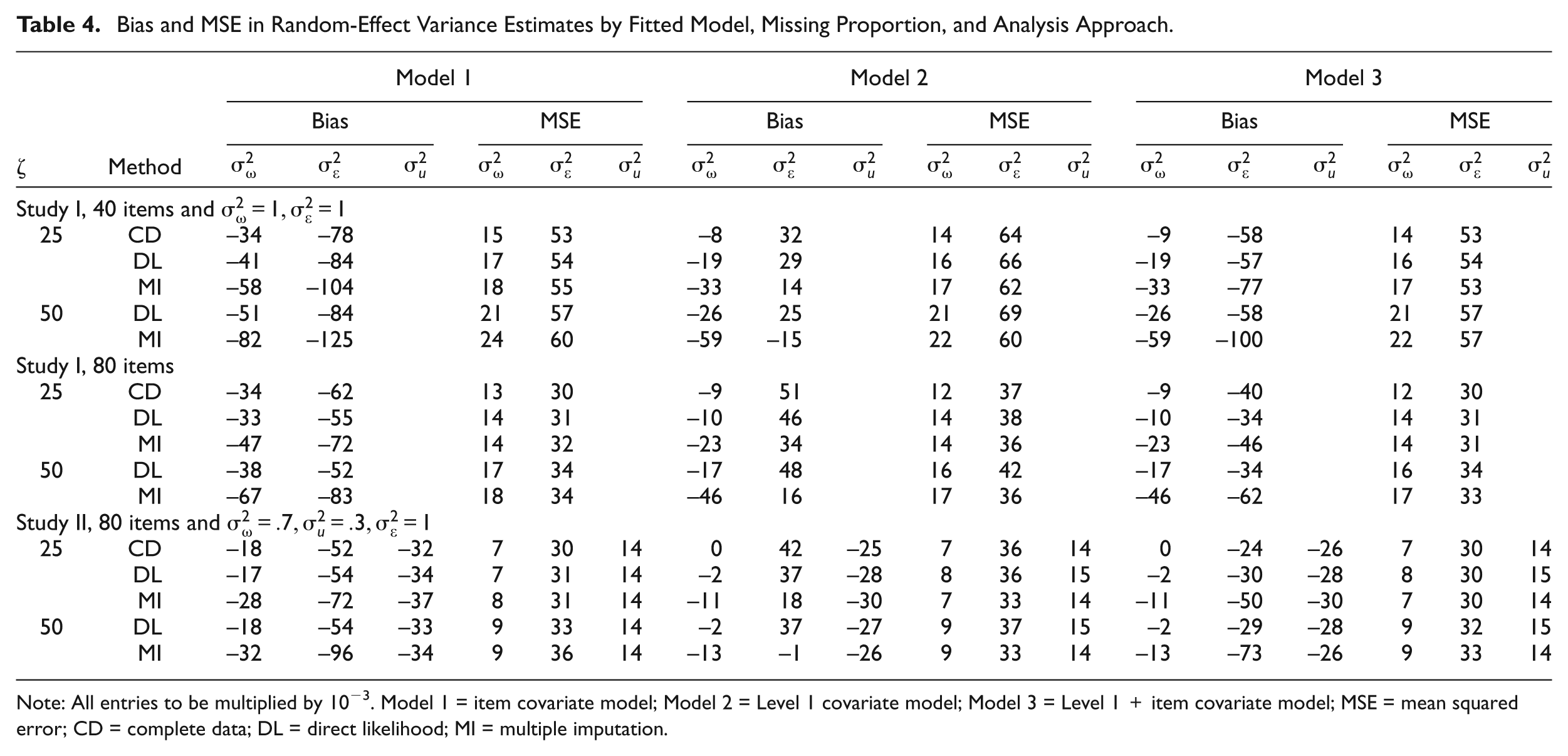
Note: All entries to be multiplied by 10−3. Model 1 = item covariate model; Model 2 = Level 1 covariate model; Model 3 = Level 1 + item covariate model; MSE = mean squared error; CD = complete data; DL = direct likelihood; MI = multiple imputation.
MSE
Table 4 shows that the obtained MSE values from both DL and MI approaches for all random effects’ variance estimates are comparable with those of the CD analysis for almost all considered conditions. The MSE values of the variance estimates for item difficulties are only slightly larger at 50% missing data. In general and compared with the CD analysis, there was a similar but slight loss of prediction accuracy for both the DL and MI analysis approaches in all the considered conditions.
Example
Assuming the MAR mechanism, a tracking-and-logging data set with a relatively large proportion of missing item scores (57%) was used to compare the DL and MI approaches. MI is implemented with different values of the number of imputations, that is, for M = 1, 3, 5, 10, and 20 to illustrate the effect of M on the estimates and standard errors of parameters of interest.
The analyzed data set was obtained from an item-based e-learning environment which was designed for students of the bachelor programs of Educational Studies, Educational Sciences, and Speech Therapy and Audiology Sciences of the University of Leuven in Belgium and offers a regression analysis module. The environment’s usage is voluntary much as students are encouraged and motivated by the authors to independently engage the exercises online at different times of their choice outside the traditional classroom-based lecture times. Each student can engage an item only once and item scores are binary coded (correct/wrong). Eighty multiple-choice exercise items were presented to students during the two semesters of the 2011/2012 academic year. One item property (item type) and one person property (course) are taken into account. In this regard, 35.5% of the items pertain to comprehension, 13.8% to knowledge, and 53.7% to practical computations. The considered data set contains only those persons (134 in number) who have got item scores on at least 5 items. Of these persons, only 8% belonged to the Educational Studies program, while 67.9% and 23.9% belonged to the bachelor programs of Educational Sciences, and Speech Therapy and Audiology Sciences. Overall, the distribution of the number of items per person is skewed to the right with a median and mean of 26 and 34 exercise items, respectively. The minimum number of persons per item is 43 with a mean of 58 and a maximum of 71.
Three explanatory IRT models—an item covariate model, a person covariate model, and a model with both covariates—were fitted to the data set. All covariates were fitted as categorical predictors. The “course” covariate includes only two dummy variables. The first dummy equals 1 for persons following bachelor of educational studies and 0 otherwise, while the second dummy variable equals 1 for persons following bachelor of educational sciences and 0 otherwise. Persons following the bachelor of speech therapy and audiology sciences were used as a reference category. Similarly, the “item type” covariate was modeled using two dummy variables with comprehension items used as a reference category. For implementation of the MI approach, similar procedures as discussed in the simulation study are followed, while the DL approach is straightforward as before. The obtained results are given in Table 5. From all DL analyses, it appears that the considered covariates are not strongly related to the missing item scores because exclusion of one covariate has little effect on the estimates of the parameters remaining in the model. However, two important observations can be noted. First, taking the DL results for the models including the covariates as a benchmark, all analyses involving M = 1 resulted in estimates of fixed effects and of the variances of random effects that are biased downward. The corresponding standard errors under M = 1 are also underestimated. Second, it can be observed that the estimates and standard errors under the MI approach are relatively stable and comparable for all analyses with M = 3, 5, 10, and 20 imputations. Moreover, all the results with M > 1 are comparable with those obtained under the DL approach.
Estimates and Standard Errors for the Models Fitted to the Empirical Example by Analysis Approach.
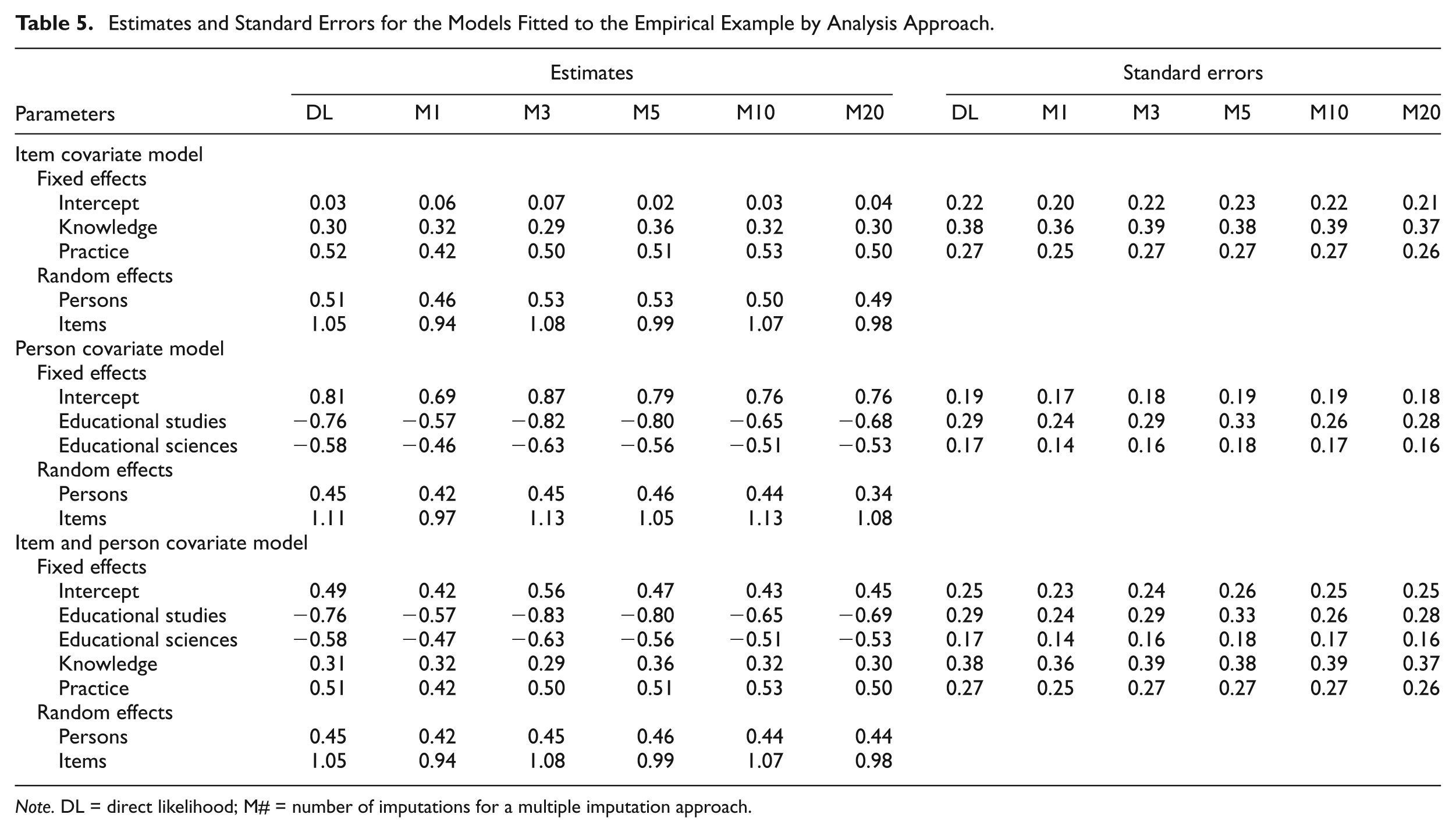
Note. DL = direct likelihood; M# = number of imputations for a multiple imputation approach.
Discussion and Conclusion
The main goal of this article was to compare the performance of a MI approach based on empirical Bayes techniques with a DL analysis when analyzing multilevel cross-classified item response data with missing binary item response scores using different explanatory IRT models, and when the model for generating multiply imputed data sets is more general than that used for analysis. The imputation model included covariates that are predictive of the outcome and are related to the missing scores, but any of these may be dropped from an analysis model of interest and still get unbiased estimates. But a similar analysis model using the DL approach can result in biased estimates. Given that the fitted IRT model is specified correctly, analyses of the fully observed data sets (CD) are assumed to give reliable estimates of the parameters of interest. Therefore, both the DL and MI approaches were considered to perform effectively if obtained results are similar to those of CD analysis.
From the simulations, it is observed that when an analysis model contained those covariates related to the missing scores, both the DL and MI approaches produced unbiased and generally similar parameter estimates of fixed effects, with MSE, standard errors (and standard deviations of the estimates), and confidence interval coverage probabilities comparable with those of a CD analysis. This is in conformity with Schafer (2003) who stated that if the user of the maximum likelihood (ML) procedure and the imputer use the same set of input data (same variables and observational units); if their models apply equivalent distributional assumptions to the variables and the relationships among them; if the sample size is large; and if the number of imputations is sufficiently large; then the results from the ML and MI procedures will be essentially identical. (p. 23)
Of course, as expected, precision of estimates tended to decline with larger proportions of missing scores—both for DL and MI analyses—and consequently, confidence intervals may not cover the true values very well.
Furthermore, these simulations illustrate that when the covariate causing missingness is not included in the analysis model, the DL approach produced biased parameter estimates of the intercept with MSE values larger than those of the CD analysis. The corresponding coverage proportions of the confidence interval are smaller than the nominal value. These observations are expected because the MAR assumption is violated in such a DL analysis. However, analyses from a similar model fitted to multiply imputed data resulted in estimates that were similar and comparable with those of the CD analysis. This illustrated the main conclusion of this article—that as long as the MAR assumption is postulated, a data set with missing item scores can first be imputed using a more general MI model, and then analysts can fit “smaller” models of their interest, even if these models do not include covariates associated with the missingness, but still arrive at similar conclusions as those of the CD analysis. Of course, these conclusions apply in principle only for the conditions considered in this study. It would be interesting to study larger missing proportions and other sample sizes. In the considered conditions, random effects’ variance parameter estimates are slightly negatively biased for the DL approach, with the MI approach posting slightly larger biases. However, the corresponding MSE estimates for both approaches are comparable with those of the CD analysis implying no or very little loss of prediction accuracy.
The empirical example illustrated that results based on M = 3, 5, 10, and 20 are generally similar in the case of a relatively large proportion of missing item scores (i.e., 57%). This further underlines the point that one can obtain reliable and efficient estimates when using a moderate number of imputations. Note that in this particular example, single value imputation resulted in biased estimates and that all standard errors were underestimated. As discussed before, this is because single-value imputations do not account for imputation uncertainty because variability induced by not knowing the missing values is ignored. Hence, this approach is generally not recommended.
The authors conclude that MI is generally desirable when the analysis and imputation approaches differ but in case they are similar, then the DL analysis is a parsimonious approach because it can be implemented with no additional programming involved, yielding similar results as those that would be obtained if the described imputation approach is employed. However, not much is known on how or whether the implemented MI model can be applied to missing covariate data, or to settings outside the scope of the current article. These are areas of possible future research.
Footnotes
Acknowledgements
The authors express kind acknowledgments to the Hercules Foundation and the Flemish Government–Department EWI for funding the Flemish Supercomputer Centre (VSC) whose infrastructure was used to carry out the simulations. They also thank two anonymous reviewers and Editor in Chief Dr. Hua-Hua Chang for their insightful comments and suggestions.
Declaration of Conflicting Interests
The author(s) declared no potential conflicts of interest with respect to the research, authorship, and/or publication of this article.
Funding
The author(s) disclosed receipt of the following financial support for the research, authorship, and/or publication of this article: Lead contributor is funded under scholarship Ref. BEURSDoc/FLOF.