Online Item Calibration for Q-Matrix in CD-CAT

Abstract

Item replenishment is important for maintaining a large-scale item bank. In this article, the authors consider calibrating new items based on pre-calibrated operational items under the deterministic inputs, noisy-and-gate model, the specification of which includes the so-called $Q$ -matrix, as well as the slipping and guessing parameters. Making use of the maximum likelihood and Bayesian estimators for the latent knowledge states, the authors propose two methods for the calibration. These methods are applicable to both traditional paper–pencil–based tests, for which the selection of operational items is prefixed, and computerized adaptive tests, for which the selection of operational items is sequential and random. Extensive simulations are done to assess and to compare the performance of these approaches. Extensions to other diagnostic classification models are also discussed.

Keywords

online calibration computerized adaptive testing diagnostic classification models

Diagnostic classification models (DCMs) are an important statistical tool in cognitive diagnosis that can be used in a number of disciplines, including educational assessment and clinical psychology (Rupp & Templin, 2008b). A key component of many DCMs is the so-called $Q$ -matrix (K. Tatsuoka, 1983), which specifies the item–attribute relationships of a diagnostic test. Various DCMs have been built around the $Q$ -matrix. One simple and widely studied example is the DINA (deterministic inputs, noisy-and-gate; see Haertel, 1989; Junker & Sijtsma, 2001) model, which is the main focus of this article. Other important models and developments can be found in DiBello, Stout, and Roussos (1995); Junker and Sijtsma (2001); Hartz (2002); C. Tatsuoka (2002); Leighton, Gierl, and Hunka (2004); von Davier (2005); Templin and Henson (2006); Chiu, Douglas, and Li (2009); K. Tatsuoka (2009); and Rupp, Templin, and Henson (2010).

Computerized adaptive testing (CAT) is a testing mode in which the item selection is sequential and individually tailored to each examinee. In particular, subsequent items are selected based on the examinee’s responses to prior items. CAT was originally proposed by Lord (1971) for item response theory (IRT) models, for which items are tailored for each examinee to “best fit” his or her ability level $θ$ , so that more capable examinees avoid receiving items that are too simple and less capable examinees avoid receiving items that are too difficult. Such individualized testing schemes perform better than do traditional exams with a prefixed selection of items because the optimal selection of testing items is subject dependent. It also leads to greater efficiency and precision than that can be achieved in traditional tests (van der Linden & Glas, 2000; Wainer et al., 1990).

For CAT under IRT settings, items are typically chosen to maximize the Fisher information (MFI; Lord, 1980; Thissen & Mislevy, 1990) or to minimize the expected posterior variance (MEPV; Owen, 1975; van der Linden, 1998). For CAT under DCM, recent developments include Xu, Chang, and Douglas (2003); Cheng (2009); and Liu, Ying, and Zhang (2013).

An important task in maintaining a large-scale item bank for CAT is item replenishment. As an item becomes exposed to more and more examinees, it needs to be replaced by new ones, for which the item-specific parameters need to be calibrated according to existing items in the bank. In CAT, online calibration is commonly used to calibrate new items (Stocking, 1988; Wainer & Mislevy, 1990). That is, to estimate the item-specific parameters, new items are assigned to examinees during their tests together with the existing items in the bank (also known as the operational items). In the literature, several online calibration methods have been developed for item-response-theory-based computerized adaptive tests for which the examinees’ latent traits are characterized by a unidimensional $θ$ . A short list of methods includes Stocking’s (1988) Method A and Method B, marginal maximum likelihood estimation with one expectation maximization (OEM) iteration (Wainer & Mislevy, 1990), marginal maximum likelihood estimation with multiple EM (MEM) iterations (Ban, Hanson, Wang, Yi, & Harris, 2001; Ban, Hanson, Yi, & Harris, 2002), the Item Analysis and Test Scoring With Binary Logistic Models (BILOG; computer program)/Prior method (Ban et al., 2001), and marginal Bayesian estimation (MBE) with Markov Chain Monte Carlo (MCMC) approach (Segall, 2003).

In the context of cognitive diagnosis, three online calibration methods, namely, Cognitive Diagnostic-Method A (CD-Method A), Cognitive Diagnostic–One EM Cycle (CD-OEM), and Cognitive Diagnostic–Multiple EM Cycles (CD-MEM), are proposed by Chen, Xin, Wang, and Chang (2012). These methods focus on the calibration of the slipping and guessing parameters, assuming the corresponding $Q$ -matrix entries are known. They are parallel to the calibration methods for IRT as described in the preceding paragraph. The CD-Method A is a natural extension of Stocking’s Method A that plugs in the knowledge state estimates. The CD-OEM and CD-MEM methods are similar to the OEM and MEM methods developed for IRT models. When the $Q$ -matrix of the new items is unknown, the joint estimation algorithm (JEA) is proposed by Chen and Xin (2011), which depends entirely on the examinees’ responses to the operational and new items to jointly calibrate the $Q$ -matrix and the slipping and guessing parameters.

In this article, the authors further extend the work of Chen et al. (2012) by considering item calibration in terms of both the $Q$ -matrix and the slipping and guessing parameters. The $Q$ -matrix is a key component in the specification of DCM and, when correctly specified, allows for the accurate calibration of the other parameters. However, its misspecification could lead to serious problems in all aspects; for example, see Rupp and Templin (2008a) for the effects of misspecification of $Q$ -matrix in DINA model. In this article, the authors extend the analysis by considering the $Q$ -matrix entries of the new items as additional item-specific parameters that are to be estimated simultaneously with the slipping and guessing parameters. Such a data-driven $Q$ -matrix also serves as a validation of the subjective item–attribute relationship specified in the initial construction of new items. The methods are different from the JEA (Chen & Xin, 2011), and a comparison is made based on simulation studies in the online appendix.

The rest of this article is organized as follows: In the next section, the authors first review existing online calibration methods of new items whose $Q$ -matrix is completely specified as well as the JEA when the $Q$ -matrix of new items is unknown and then propose new approaches that simultaneously calibrate both the $Q$ -matrix and the slipping and guessing parameters. In the last section, conclusions drawn from the simulation studies as well as further discussions are provided. Simulation studies are included in an online appendix comparing the performance among various methods.

Calibration for Cognitive Diagnosis

Problem Setting

Throughout this article, the authors consider an item bank containing a sufficiently large number of operational items whose parameters have already been calibrated. There are $m$ additional items whose parameters are to be calibrated. Both the operational items and the new items are associated with at most $k$ attributes. The calibration procedure is carried out as follows: Each examinee responds to $C$ operational items and $D$ new items. In a traditional paper–pencil test, the operational items assigned to each examinee are identical. In a computerized adaptive test, the item selections are tailored to each examinee. The proposed calibration procedure does not particularly depend on the testing mode. Furthermore, for $j = 1, \dots, m$ , let $n_{j}$ be the total number of examinees responding to the new item $j$ , $R_{j} = (R_{1, j}, \dots, R_{n_{j}, j})$ be the vector of responses to new item $j$ , $r_{i} = (r_{i, 1}, \dots, r_{i, C})$ be the response vector of examinee $i$ to the $C$ operational items.

The DINA model that is commonly used in educational assessment is assumed. Under the DINA model, the knowledge state is described by a $k$ dimensional vector with zero–one entries. Specifically, examinee $i$ ’s knowledge state is given by a vector $α_{i} = (α_{i}^{1}, \dots, α_{i}^{k})$ , where $α_{i}^{l}$ is either one or zero, indicating the presence or absence, respectively, of the $l$ th skill. In this article, the terms knowledge state, attribute profile, and skill are exchangeable and denoted by vector $α$ . The DINA model assumes a conjunctive relationship among the skills. Consider an item and let $q = (q^{1}, \dots, q^{k})$ be the corresponding row vector in the $Q$ -matrix, where $q^{l} = 1$ indicates that the correct response of this item requires the presence of attribute $l$ . Furthermore, the DINA model assumes that an examinee is capable of providing a correct answer to this item when the examinee possesses all the required skills. Thus, the authors define the ideal response of an examinee of attribute $α$ to an item of row vector $q$ as

ξ (q, α) = Π_{l = 1}^{k} {(α^{l})}^{q^{l}} = 1 (α^{l} \geq q^{l} forall l = 1, \dots, k) .

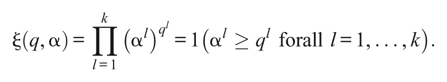
The response distribution is then defined as

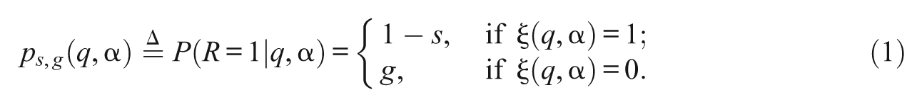
p_{s, g} (q, α) \overset{Δ}{=} P (R = 1 | q, α) = {\begin{matrix} 1 - s, & if ξ (q, α) = 1; \\ g, & if ξ (q, α) = 0 . \end{matrix}

The parameter $s$ is known as the slipping parameter, representing the probability of an incorrect response to the item for examinees who are capable of answering correctly, and $g$ is known as the guessing parameter, representing the probability of a correct response for those who are not capable.

Suppose that an examinee’s responses to a set of operational items $r = (r_{1}, \dots, r_{C})$ have been collected. $q_{i}$ , $s_{i}$ , and $g_{i}$ is used to denote the row vectors of the $Q$ -matrix, the slipping parameters, and the guessing parameters, respectively. In the setting of CAT, the selection of items is possibly random in that the specific choice of $(q_{j}, s_{j}, g_{j})$ typically depends on the examinee’s previous responses $(r_{1}, \dots, r_{j - 1})$ . Here, the assumption is made that the sequential selection rule of subsequent items only depends on the responses $(r_{1}, \dots, r_{j - 1})$ and does not depend on any other information of the knowledge state $α$ . 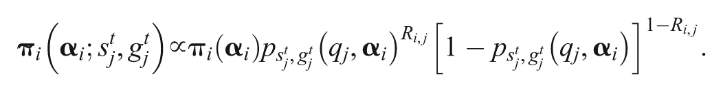Therefore, the observation of item selections does not provide further information on the knowledge state. Based on this, the likelihood function of knowledge state can be written down as

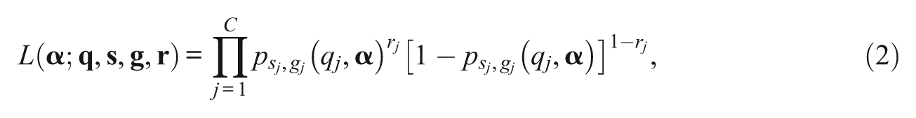
L (α; q, s, g, r) = Π_{j = 1}^{C} p_{s_{j}, g_{j}} {(q_{j}, α)}^{r_{j}} {[1 - p_{s_{j}, g_{j}} (q_{j}, α)]}^{1 - r_{j}},

where $q = (q_{1}, \dots, q_{C})$ , $s = (s_{1}, \dots, s_{C})$ , and $g = (g_{1}, \dots, g_{C})$ . Under the Bayesian framework, inferences about $α$ can be made based on its posterior distribution

π (α | q, s, g, r) \propto L (α; q, s, g, r) π (α),

where $π (α)$ is the prior distribution and the symbol “ $\propto$ ” reads as “is proportional to.”

Existing Methods for Online Calibration for CD-CAT With a Known Q-Matrix

The authors begin with a brief review of the three online calibration methods proposed in Chen et al. (2012). The purpose of these methods is to estimate the slipping and guessing parameters $s$ and $g$ when the corresponding $Q$ -matrix is specified (known). For a specific new item $j$ , suppose that there are $n_{j}$ examinees responding to the item. The first method, which is known as CD-Method A, considers the estimated the knowledge state ${\hat{α}}_{i}$ as the true, for $i = 1, \dots, n_{j}$ . Estimates of the slipping and guessing parameter are obtained via the maximum likelihood estimator (MLE) that solves the following normal equations:

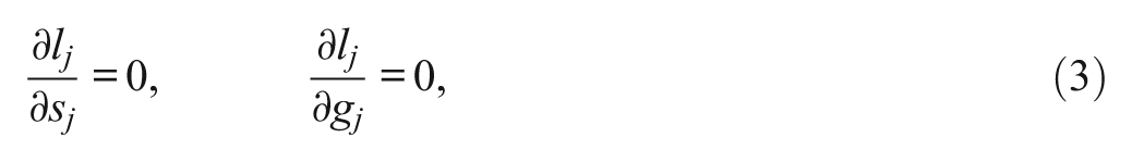
\frac{\partial l_{j}}{\partial s_{j}} = 0, \frac{\partial l_{j}}{\partial g_{j}} = 0,

where $l_{j} (q_{j}, s_{j}, g_{j}) = log (Π_{i = 1}^{n_{j}} p_{s_{j}, g_{j}} {(q_{j}, {\hat{α}}_{i})}^{R_{i, j}} {[1 - p_{s_{j}, g_{j}} (q_{j}, {\hat{α}}_{i})]}^{1 - R_{i, j}})$ and $q_{j}$ is the row vector of $Q$ -matrix for the new item. The parameters $s_{j}$ and $g_{j}$ enter the likelihood through the probability $p_{s_{j}, g_{j}} (q_{j}, {\hat{α}}_{j})$ defined as in Equation 1.

The second method, which is known as the CD-OEM, considers the uncertainty contained in the estimates ${\hat{α}}_{i}$ by incorporating the entire posterior distribution and uses a single cycle of an EM-type algorithm to obtain the marginal maximum likelihood estimate. In particular, for a given new item $j$ , the CD-OEM method first takes one E-step with respect to the posterior distribution of the knowledge states, given the responses to the operational items. Next, the M-step maximizes the logarithm of the expected likelihood.

The third method, CD-MEM, is an extension of the CD-OEM method. It increases the number of EM cycles until some convergence criterion is satisfied. Specifically, the first EM cycle of the CD-MEM method is identical to the CD-OEM method, and the new item parameter estimates obtained from the first EM cycle are regarded as the initial new item parameters of the second EM cycle. From the second EM cycle onward, the CD-MEM method utilizes the responses from both the operational and new items to obtain the posterior distribution of the knowledge states for the E-step. The M-step is the same as that of the CD-OEM method, except that the likelihood is marginalized with respect to the posterior distribution given responses to both the operational and the new items. One advantage of the CD-MEM method is that it fully utilizes the information from both the operational and the new items.

The JEA

When the $Q$ -matrix is unknown, the JEA (Chen & Xin, 2011) estimates both the $Q$ -matrix and the slipping and guessing parameters of the new items. The algorithm, as an extension of CD-Method A, treats the estimated knowledge state ${\hat{α}}_{i}$ as the true. In particular, the posterior mode is used to estimate the examinees’ knowledge states based on their responses to the operational items. The algorithm calibrates one item at a time. For a specific item $j$ , the JEA optimizes $l_{j} (q_{j}, s_{j}, g_{j})$ with respect to $q_{j}$ given $(s_{j}, g_{j})$ and optimizes $l_{j} (q_{j}, s_{j}, g_{j})$ with respect to $(s_{j}, g_{j})$ given $q_{j}$ iteratively until convergence is reached according to some criterion. The advantage of this algorithm is that it is easy to implement.

Online Calibration of Q-Matrix

In this section, the authors consider the new item calibration under the DINA model. To motivate the methods, they first consider a hypothetical situation in which the slipping and guessing parameters are known and the $Q$ -matrix is the only unknown parameter in need of calibration. They then consider calibrating both the $Q$ -matrix and the slipping and guessing parameters. For this, they first present an approach that calibrates one item at a time and then a second approach that deals that multiple items simultaneously. They discuss the advantages in efficiency of the latter over the former.

Calibration with known slipping and guessing parameters

Without loss of generality, indices can always be rearranged so that a new item $j$ is assigned to examinees $1, \dots, n_{j}$ . For examinee $i$ , $π_{i} (α_{i})$ is used to denote the posterior distribution of the knowledge state given his or her responses to the operational items. For a new item with $Q$ -matrix row vector $q_{j}$ , the posterior predictive distribution of a particular response pattern $R_{i, j}$ is

p_{i} (q_{j}, s_{j}, g_{j}) \overset{Δ}{=} P (R_{i, j} = 1 | q_{j}, s_{j}, g_{j}) = \sum_{α} π_{i} (α) p_{s_{j}, g_{j}} (q_{j}, α), i = 1, \dots, n_{j},

where $p_{s, g}$ is defined as in Equation 1. Therefore, the likelihood function is written down based on the responses of $n_{j}$ examinees as

L_{j} (q_{j}, s_{j}, g_{j}) = Π_{i = 1}^{n_{j}} p_{i} {(q_{j}, s_{j}, g_{j})}^{R_{i, j}} {[1 - p_{i} (q_{j}, s_{j}, g_{j})]}^{1 - R_{i, j}} .

Note that here both $s_{j}$ and $g_{j}$ are assumed to be known. An estimate of $q_{j}$ can be obtained through the MLE; that is,

{\hat{q}}_{j} = arg max_{q_{j}} L_{j} (q_{j}, s_{j}, g_{j}) .

For the computation of the above MLE, notice that there are $2^{k} - 1$ possible $q_{j}$ s. The authors simply compute $L_{j} (q_{j}, s_{j}, g_{j})$ for each possible $q_{j}$ and choose the maximum. This is not much of a computational burden and can be carried out easily for $k$ less than 10.

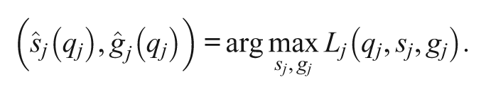
Calibration for a single item with unknown slipping and guessing parameters

The authors now proceed to the more realistic situation when $s_{j}$ and $g_{j}$ are also unknown and need to be calibrated along with $q_{j}$ . As in the previous discussion, they still work with the likelihood function (Equation 4). The MLE is then defined as

({\hat{q}}_{j}, {\hat{s}}_{j}, {\hat{g}}_{j}) = arg max_{q_{j}, s_{j}, g_{j}} L_{j} (q_{j}, s_{j}, g_{j}) .

Because the likelihood here is a function of both discrete $q_{j}$ and continuous $(s_{j}, g_{j})$ , its maximization is not easy to carry out numerically. The authors’ approach is to break it down into two steps. In Step 1, for each possible $q_{j}$ value, they compute the maximized likelihood estimates with respect to $s_{j}$ and $g_{j}$ ; that is,

({\hat{s}}_{j} (q_{j}), {\hat{g}}_{j} (q_{j})) = arg max_{s_{j}, g_{j}} L_{j} (q_{j}, s_{j}, g_{j}) .

This step can be carried out by the EM algorithm that is an iterative algorithm. More precisely, the algorithm starts from an initial value $(s_{j}^{0}, g_{j}^{0})$ . Let $(s_{j}^{t}, g_{j}^{t})$ be the parameter values at iteration $t$ . The evolution from $(s_{j}^{t}, g_{j}^{t})$ to $(s_{j}^{t + 1}, g_{j}^{t + 1})$ consists of an E-step and an M-step. In the E-step, the posterior distribution of $α_{i}$ given a particular response $R_{i, j}$ to the new item is obtained by

{\tilde{π}}_{i} (α_{i}; s_{j}^{t}, g_{j}^{t}) \propto π_{i} (α_{i}) p_{s_{j}^{t}, g_{j}^{t}} {(q_{j}, α_{i})}^{R_{i, j}} {[1 - p_{s_{j}^{t}, g_{j}^{t}} (q_{j}, α_{i})]}^{1 - R_{i, j}} .

Then the expected log likelihood

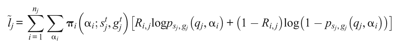
{\tilde{l}}_{j} = \sum_{i = 1}^{n_{j}} \sum_{α_{i}} {\tilde{π}}_{i} (α_{i}; s_{j}^{t}, g_{j}^{t}) [R_{i, j} log p_{s_{j}, g_{j}} (q_{j}, α_{i}) + (1 - R_{i, j}) log (1 - p_{s_{j}, g_{j}} (q_{j}, α_{i}))]

is computed. In the M-step, the parameters are updated by $(s_{j}^{t + 1}, g_{j}^{t + 1})$ maximizing ${\tilde{l}}_{j}$ with respect to $(s_{j}, g_{j})$ . Equivalently, $(s_{j}^{t + 1}, g_{j}^{t + 1})$ solves the normal equations

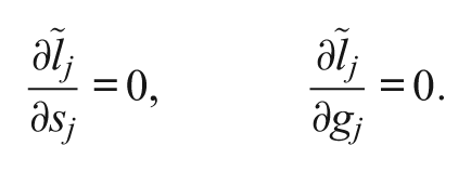
\frac{\partial {\tilde{l}}_{j}}{\partial s_{j}} = 0, \frac{\partial {\tilde{l}}_{j}}{\partial g_{j}} = 0 .

The algorithm iterates the E-step and the M-step until convergence, as signaled by some precision rule. The simulation study shows that the convergence of the EM algorithm is very fast and it typically takes only a few steps.

In Step 2, the authors then obtain ${\hat{q}}_{j}$ as the maximizer of the profile likelihood function; that is

{\hat{q}}_{j} = arg max_{q_{j}} L_{j} (q_{j}, {\hat{s}}_{j} (q_{j}), {\hat{g}}_{j} (q_{j})) .

Once ${\hat{q}}_{j}$ has been computed, the estimates of the slipping and the guessing parameter are then given as ${\hat{s}}_{j} ({\hat{q}}_{j})$ and ${\hat{g}}_{j} ({\hat{q}}_{j})$ .

The preceding approach calibrates a single item at a time and it is a natural procedure when each examinee is given only a single new item. It is also applicable when multiple new items are assigned to an examinee for which the authors focus on a particular new item for its calibration and ignore all others. They call this method the single-item estimation (SIE) method. Under the setting of Simulation Study 1 in the online appendix, the calibration of 12 new items in one simulation using the SIE method takes approximately 3.3 s in R (version 2.13.1) on a 2.5 GHz laptop running Windows 7 Professional.

Both JEA and SIE calibrate a single item at a time. However, unlike JEA, the SIE method takes the uncertainty of the knowledge state estimates into account. Instead of plugging in the estimates of the knowledge states, the posterior distributions are used in SIE to calculate the posterior predictive distribution of response patterns. In other words, more information from examinees’ responses to the operational items is utilized in the SIE method. Therefore, SIE is expected to be more efficient than is JEA in estimating the $Q$ -matrix and the slipping and guessing parameters, especially when the estimates of examinees’ knowledge states are not accurate and when the sample size is relatively large.

Calibration of multiple items

In this section, the authors further propose a calibration procedure to calibrate multiple items simultaneously. To start with, they would like to explain why simultaneous calibration could improve the efficiency of the calibration method described in the preceding section. For the calibration of new item-specific parameters, it is clear from Equation 2 that ideally the authors would like to have examinees’ knowledge states known. However, this is practically infeasible. Thus, they make use of the operational items to first get estimates of examinees’ knowledge states and then, based on the estimated knowledge states as characterized by their posterior distributions, they proceed to calibrating the new items. Therefore, the more accurate the information about the knowledge states is, the better the calibration will be. The idea of simultaneous calibration is to borrow the information contained in the responses to new items so as to further improve the measurement of the unknown knowledge states. One issue with this idea is that using information from a new item whose parameters (especially $Q$ ) have not been adequately calibrated may have an adverse effect on the measurement of examinees’ knowledge states. Therefore, it is necessary to select the new items with sufficient calibration accuracy (based on the data). In this connection, the authors introduce an item-specific statistic $η_{j}$ to quantify the accuracy of the estimation of $q_{j}$ . They call $η_{j}$ the confidence index that represents the confidence in the fit of $q_{j}$ . To start with, an estimate is obtained for each $q_{j}$ separately via Equation 5 and denote it by ${\hat{q}}_{j}$ . The confidence index is defined as

η_{j} \overset{Δ}{=} log (max_{q_{j}, s_{j}, g_{j}} L_{j} (q_{j}, s_{j}, g_{j})) - log (max_{q_{j} \neq {\hat{q}}_{j}, s_{j}, g_{j}} L_{j} (q_{j}, s_{j}, g_{j})) .

If $({\tilde{q}}_{j}, {\tilde{s}}_{j}, {\tilde{g}}_{j}) = argma x_{q_{j} \neq {\hat{q}}_{j}, s_{j}, g_{j}} L_{j} (q_{j}, s_{j}, g_{j})$ is defined, then ${\tilde{q}}_{j}$ is the second most probable $q$ vector for item $j$ according to the likelihood. In other words, the statistic $η_{j}$ is the logarithm of the likelihood ratio between ${\hat{q}}_{j}$ and ${\tilde{q}}_{j}$ , the two most probable $Q$ s for item $j$ . The larger $η_{j}$ is, the more confident we are in the fit of ${\hat{q}}_{j}$ .

Suppose that there are $m$ new items to be calibrated. A new method is introduced which is built upon the SIE method and simultaneously calibrates all the new items’ parameters. It is described by the following algorithm:

Calibrate the unknown parameters of new items $1, 2, \dots, m$ , one at a time via the procedure in the preceding section and obtain $({\hat{q}}_{j}, {\hat{s}}_{j}, {\hat{g}}_{j}, η_{j})$ , for $j = 1, 2, \dots, m$ .

The new items with $η_{j}$ larger than a threshold $λ$ are selected, and sorted in a decreasing order according to $η_{j}$ . Suppose that there are $l$ items selected, denoted by $j_{1}, \dots, j_{l}$ . These items are viewed as “good” ones for which the authors are confident in ${\hat{q}}_{j}$ s. $λ$ is chosen as half of the 95% quantile of the $χ^{2}$ distribution with one degree of freedom. Although the asymptotic distribution of $2 η_{j}$ is not really $χ^{2}$ distributed and is unclear, simulation study shows that this $λ$ works well empirically, and it can be tuned in applications.

New item $j_{1}$ is treated as an additional operational item and the calibrated parameters are treated $({\hat{q}}_{j_{1}}, {\hat{s}}_{j_{1}}, {\hat{g}}_{j_{1}})$ as the true. Then, the knowledge state posterior distributions is updated for those examinees who responded to new item $j_{1}$ , given their responses to both the operational items and this new item $j_{1}$ . With the new knowledge state posterior distributions, the authors proceed to recalibrate new item $j_{2}$ by applying the procedure in the preceding section, and update $({\hat{q}}_{j_{2}}, {\hat{s}}_{j_{2}}, {\hat{g}}_{j_{2}})$ .

$l + 1 .$ New items $j_{1}, \dots, j_{l - 1}$ are treated as operational items and their calibrated parameters as the true. With new knowledge state posterior distributions by further conditioning on the responses to these $l - 1$ new items, the authors apply the procedure in the preceding section to calculate $({\hat{q}}_{j_{l}}, {\hat{s}}_{j_{l}}, {\hat{g}}_{j_{l}}, η_{j_{l}})$ and update the knowledge state posterior distributions.

Now, all the $l$ selected new items except item $j_{1}$ have been recalibrated, and they all serve as the operational items. The authors continue the procedure by recalibrating the parameters of new items not selected in Step 2.

$l + 2 .$ Using the current posterior distributions of knowledge states given the responses to the operational items and the “good” items, recalibrate the parameters of items not selected in Step 2 one at a time, according to the procedure in the preceding section.

$l + 3 .$ With the updated $({\hat{q}}_{j}, {\hat{s}}_{j}, {\hat{g}}_{j}, η_{j})$ , for $j = 1, 2, \dots, m$ , the items with their $η_{j}$ s larger than the threshold are selected. If the selected items are the same as those selected in Step 2, the algorithm ends. Otherwise, sort the selected items according to the new $η_{j}$ s from the largest to the smallest, reset the posterior distributions of knowledge states to the one in Step 1 (from the responses to the original operational items), and go to Step 3.

The algorithm ends when the selected “good” estimates do not change in two rounds, which intuitively means that all the “good” items have been utilized to refine the estimation of examinees’ knowledge states. Then, the authors report the calibrated item parameter values. They refer to this method as simultaneous item estimation (SimIE) method. Under the setting of Simulation Study 1 in the online appendix, the calibration of 12 new items using the SimIE method takes approximately 7.3 s in R (version 2.13.1) on a 2.5 GHz laptop running Windows 7 Professional.

Conclusion and Further Discussions

In this article, the authors propose new item calibration methods for the $Q$ -matrix, a key element in cognitive diagnosis, as well as the slipping and guessing parameters. These methods extend the work of Chen et al. (2012) and are compared with the JEA proposed in Chen and Xin (2011). Under the setting of Study 1 in the online appendix, the results show that the proposed SIE and SimIE methods perform better than the JEA method in the calibration of the $Q$ -matrix as well as the estimation of slipping and guessing parameters. In addition, JEA is sensitive to the accuracy of the estimation of examinees’ knowledge states. The simulation results in Study 1 also show that the SimIE method is superior to the SIE method for the calibration of the $Q$ -matrix as well as the estimation of slipping and guessing parameters. As all three methods can be implemented without much computational burden, the SimIE method is therefore preferred. From the results of Study 2 in the online appendix, all three methods tend to estimate the item parameters more accurately as the sample size becomes larger. In particular, when the sample size is 1,600, under the simulation setting, both the SIE and SimIE methods correctly calibrate the $Q$ -matrix with probability close to 1, and estimate the slipping and guessing parameters with an acceptable accuracy (based on the root mean square error [RMSE] values).

Furthermore, the authors introduce the confidence index $η$ to evaluate the goodness-of-fit for a new item. When $Q$ is specified, the estimation accuracy of the slipping and guessing parameters is quantified by the observed Fisher information based on the likelihood function. When $Q$ is also unknown, the confidence index plays a similar role of the observed Fisher information, as $Q$ is discrete. Thus, the index itself is of interest in online calibration and, along with the observed Fisher information of the slipping and guessing parameters, summarizes the estimation accuracy of item parameters for a new item. Based on it, a decision may be made as to whether the calibration is sufficiently accurate.

There are a number of theoretical issues which require attention. For instance, under what circumstances can the $Q$ -matrix of the new items be consistently estimated? When can the slipping and guessing parameters be consistently estimated? The authors provide a brief discussion on this issue. Given a known $Q$ -matrix, the identifiability of the slipping and the guessing parameters can be checked by computing the Fisher information with respect to these two parameters. Then, the most important and interesting task is to ensure the identifiability of the $Q$ -matrix. Generally speaking, to consistently calibrate all possible $Q$ -matrices, we typically require the following knowledge state patterns exist in the population. For each dimension of the knowledge state $α^{l}$ , there exist a nonzero proportion of examinees who only master $α^{l}$ and do not master any other skills. $e_{l} = (0, \dots, 0, 1, 0, \dots, 0)$ is used to denote such a knowledge state vector. Missing one or a few such kind of $e_{l}$ s will affect the identification of certain patterns (not all) of $Q$ -matrix.

The preceding discussion assumes complete and accurate specification of the knowledge state of each examinee. Under the current setting, the knowledge states are not directly observed and are estimated through the responses to the operational items. Therefore, an important issue is the selection of operational items through which enough information about the knowledge states can be obtained. The authors would like to emphasize that the number of operational items responded to by each examinee is limited. Therefore, it is not required (and it is not necessary) that the knowledge state of each examinee is identified very accurately. However, the number of examinees is required to be reasonably large. Even if each of them provides a small amount of information, the new items eventually can be calibrated accurately with a sufficiently large number of people. An important issue for future study is to clarify requirements on the operational items to ensure the consistent calibration of the new item.

It is observed from both simulation studies in the online appendix that the calibration accuracy varies for different $Q$ s. For example, in Study 1, the estimation accuracy (of $Q$ ) varies for different items is observed. There are at least two aspects affecting the estimation accuracy. The first is the specific value of the slipping and guessing parameters; generally, the smaller the slipping and guessing parameters are, the easier it is to calibrate the $Q$ . This is intuitively easy to understand, because the slipping and guessing behavior introduces noise which makes the signal (the $Q$ pattern) harder to recover. The second aspect is related to the knowledge state population. For example, looking at new Items 5 and 6 from Study 1, although Item 5 has greater slipping and guessing parameters than does Item 6, the calibration of $Q$ for Item 5 is much better than that of Item 6 according to the corresponding item-specific misspecification rate (IMR) values in Tables 2 and 3 in the online appendix. Note that $q_{5} = (0, 1, 0, 0, 0)$ and $q_{6} = (1, 0, 1, 0, 1)$ . Considering the way the population is generated, almost half of the examinees are capable of solving Item 5, while only $12.5 %$ examinees are capable of solving Item 6. In other words, for Item 5, the examinees who are able to solve it and those who are not able to are balanced, while this is not the case for Item 6. Naturally, this leads to a design problem for how to adaptively assign new items to examinees according to both the current calibration of the new items and the current measurement of the examinees. This becomes extremely important under the situation that the number of examinees is also limited and also would like to optimize the calibration of all new items.

The current calibration procedure was developed under the DINA model. It is worth pointing out that this method can be extended without difficulty to other core DCMs, such as DINO (deterministic input, noisy-or-gate), NIDA (noisy inputs, deterministic-and-gate), NIDO (noisy input, deterministic-or-gate) model, and so on (see Rupp et al., 2010). To understand this, core DCMs can be viewed as special cases of log-linear models and latent classes and different constraints on model parameters (Henson, Templin, & Willse, 2009). When calibrating a single item under a log-linear model with latent classes, Step 2 in the SIE procedure does not change. More specifically, once the auxiliary model parameters are profiled out, ${\hat{q}}_{j}$ is obtained by finding the $Q$ that has the maximum profile likelihood. Step 1 may vary because the EM algorithm may not be realistically feasible for some models. However, the MCMC approach can be applied to estimate auxiliary model parameters when the EM algorithm is not feasible, although it is slower than the EM algorithm; see Chapter 11, Rupp et al. (2010). Furthermore, the SimIE method can also be generalized to other core DCMs.

The current calibration procedure works under a fixed and known dimension for the latent classes. In practice, a new exam problem, though designed to measure the same set of attributes as the operational items, may possibly be related to additional new attributes. To incorporate this new structure, more column(s) would need to be added to the existing $Q$ -matrix. Another instance that would necessitate additional dimensions is as follows. Suppose that all the operational items require some attribute. Correspondingly, there is one column in $Q$ containing all ones. Such columns are usually removed and the absence of such an attribute is ascribed to the slipping parameter. If a new item does not need this extra attribute required by all the operational items, then the removed column should be restored to maintain the correctness. In addition, the slipping and guessing parameters of the operational items need to be recalibrated according to this new $Q$ -matrix; in particular, part of the slipping probability is explained by the absence of this extra attribute. Thus, a testing mechanism needs to be developed, so as to determine whether an extra dimension should be added to the existing $Q$ -matrix during the course of online calibration.

Footnotes

Acknowledgements

The authors are very grateful to the editors and reviewers for providing valuable comments.

Declaration of Conflicting Interests

The author(s) declared no potential conflicts of interest with respect to the research, authorship, and/or publication of this article.

Funding

The author(s) disclosed receipt of the following financial support for the research, authorship, and/or publication of this article: This research is supported in part by NSF CMMI-1069064, NSF SES-1323977, and NIH R37GM047845.

Supplemental Material

The online appendix is available at

References

Ban

Hanson

Wang

Harris

(2001). A comparative study of on-line pretest item—Calibration/scaling methods in computerized adaptive testing. Journal of Educational Measurement, 38, 191-212.

Ban

Hanson

Harris

(2002). Data sparseness and on-line pretest item calibration-scaling methods in CAT. Journal of Educational Measurement, 39, 207-218.

Chen

Xin

(2011, April). Item replenishing in cognitive diagnostic computerized adaptive testing. Paper presented at the annual meeting of the National Council on Measurement in Education, New Orleans, LA.

Chen

Xin

Wang

Chang

H.-H.

(2012). Online calibration methods for the DINA model with independent attributes in CD-CAT. Psychometrika, 77, 201-222.

Cheng

(2009). When cognitive diagnosis meets computerized adaptive testing: CD-CAT. Psychometrika, 74, 619-632.

Chiu

Douglas

(2009). Cluster analysis for cognitive diagnosis: Theory and applications. Psychometrika, 74, 633-665.

DiBello

Stout

W. F.

Roussos

(1995). Unified cognitive/psychometric diagnostic assessment likelihood-based classification techniques. In Nichols

Chipman

Brennen

(Eds.), Cognitively diagnostic assessment (pp. 361-389). Hillsdale, NJ: Erlbaum.

Haertel

(1989). Using restricted latent class models to map the skill structure of achievement items. Journal of Educational Measurement, 26, 301-321.

Hartz

(2002). A Bayesian framework for the unified model for assessing cognitive abilities: Blending theory with practicality (Doctoral dissertation). University of Illinois, Urbana–Champaign.

10.

Henson

Templin

Willse

(2009). Defining a family of cognitive diagnosis models using log-linear models with latent variables. Psychometrika, 74, 191-210.

11.

Junker

Sijtsma

(2001). Cognitive assessment models with few assumptions, and connections with nonparametric item response theory. Applied Psychological Measurement, 25, 258-272.

12.

Leighton

J. P.

Gierl

M. J.

Hunka

S. M.

(2004). The attribute hierarchy model for cognitive assessment: A variation on Tatsuoka’s rule-space approach. Journal of Educational Measurement, 41, 205-237.

13.

Liu

Ying

Zhang

(2013). A rate function approach to the computerized adaptive testing for cognitive diagnosis. Unpublished manuscript.

14.

Lord

F. M.

(1971). Robbins-Monro procedures for tailored testing. Educational and Psychological Measurement, 31, 3-31.

15.

Lord

F. M.

(1980). Applications of item response theory to practical testing problems. Hillsdale, NJ: Erlbaum.

16.

Owen

R. J.

(1975). Bayesian sequential procedure for quantal response in context of adaptive mental testing. Journal of the American Statistical Association, 70, 351-356.

17.

Rupp

Templin

(2008a). The effects of Q-matrix misspecification on parameter estimates and classification accuracy in the DINA model. Educational and Psychological Measurement, 68, 78-96.

18.

Rupp

Templin

(2008b). Unique characteristics of diagnostic classification models: A comprehensive review of the current state-of-the-art. Measurement: Interdisciplinary Research and Perspective, 6, 219-262.

19.

Rupp

Templin

Henson

R. A.

(2010). Diagnostic measurement: Theory, methods, and applications. New York, NY: Guilford Press.

20.

Segall

D. O.

(2003, April). Calibrating CAT pools and online pretest items using MCMC methods. Paper presented at the annual meeting of the National Council on Measurement in Education, Chicago, IL.

21.

Stocking

M. L.

(1988). Scale drift in on-line calibration (Research Rep. 88-28). Princeton, NJ: Educational Testing Service.

22.

Tatsuoka

(2002). Data-analytic methods for latent partially ordered classification models. Journal of the Royal Statistical Society: Series C (Applied Statistics), 51, 337-350.

23.

Tatsuoka

(1983). Rule space: An approach for dealing with misconceptions based on item response theory. Journal of Educational Measurement, 20, 345-354.

24.

Tatsuoka

(2009). Cognitive assessment: An introduction to the rule space method. Florence, KY: Routledge.

25.

Templin

Henson

(2006). Measurement of psychological disorders using cognitive diagnosis models. Psychological Methods, 11, 287-305.

26.

Thissen

Mislevy

R. J.

(1990). Testing algorithms. In Wainer

Dorans

N. J.

Flaugher

Green

B. F.

Mislevy

R. J.

Steinberg

Thissen

(Eds.), Computerized adaptive testing: A primer (pp. 103-134). Hillsdale, NJ: Erlbaum.

27.

van der Linden

W. J.

(1998). Bayesian item-selection criteria for adaptive testing. Psychometrika, 63, 201-216.

28.

van der Linden

W. J.

Glas

C. A.

(2000). Computerized adaptive testing: Theory and practice. Boston, MA: Kluwer.

29.

von Davier

(2005). A general diagnostic model applied to language testing data (ETS Technical Report No. RR-05-16). Princeton, NJ: Educational Testing Service.

30.

Wainer

Dorans

Green

Steinberg

Flaugher

Mislevy

Thissen

(1990). Computerized adaptive testing: A primer. Hillsdale, NJ: Erlbaum.

31.

Wainer

Mislevy

R. J.

(1990). Item response theory, item calibration, and proficiency estimation. In Wainer

Dorans

N. J.

Flaugher

Green

B. F.

Mislevy

R. J.

Steinberg

Thissen

(Eds.), Computerized adaptive testing: A primer (pp. 65-101). Hillsdale, NJ: Erlbaum.

32.

Chang

H.-H.

Douglas

(2003, April). A simulation study to compare CAT strategies for cognitive diagnosis. Paper presented at the annual meeting of the American Educational Research Association, Chicago, IL.

Supplementary Material

Please find the following supplemental material available below.

For Open Access articles published under a Creative Commons License, all supplemental material carries the same license as the article it is associated with.

For non-Open Access articles published, all supplemental material carries a non-exclusive license, and permission requests for re-use of supplemental material or any part of supplemental material shall be sent directly to the copyright owner as specified in the copyright notice associated with the article.

0.00 MB

0.20 MB