A Power Formula for the SIBTEST Procedure for Differential Item Functioning

DIF and SIBTEST

Consider a test of length I with the first m items being the anchor items and the remaining I−m items being the studied items. Let U _i be the score for item i , X = ∑ i = 1 m U i be the total score for the anchor items, and Y = ∑ i = m + 1 I U i be the total score for the studied items. Let Y ¯ gk be the average score of the studied items for all group g (g = R or F; R for the reference group and F for the focal group) examinees for which X = k. Let N_R and N_F be the number of examinees in the reference and the focal groups, respectively, and N = N_R+N_F be the total sample size. An intuitive local measure for DIF is

d k = Y ¯ R k − Y ¯ F k , k = 0 , … , m ,

the group difference on the studied items among examinees with the same observed matching score on the anchor items. If the studied items have no DIF, one would expect d k ≈ 0 . A global DIF statistic can be defined by the weighted sum of the local group differences by

β ^ = ∑ k = 0 m p k d k = ∑ k = 0 m p k ( Y ¯ R k − Y ¯ F k ) ,

where p k = N k / N is the proportion of examinees (from the reference and focal groups pooled together) getting score X = k . A standardized version of β ^ is defined by

B = β ^ σ ^ ( β ^ ) ,

where

σ ^ ( β ^ ) = [ ∑ k = 0 m p k 2 ( σ ^ 2 ( Y | k , R ) N R k + σ ^ 2 ( Y | k , F ) N F k ) ] 1 2

is the standard error of the estimator β ^ , and σ ^ 2 ( Y | k , g ) is the sample variance of the studied item scores for examinees in group g (R or F) with matching score X = k. However, under the null hypothesis that E R ( Y | θ ) = E F ( Y | θ ) for all θ, and when there is difference in the two latent trait distributions (or impact, f R ( θ ) ≠ f F ( θ ) ), B will lead to an inflated Type I error rate because the true asymptotic distribution is no longer N(0,1) (DeMars, 2010; Roussos & Stout, 1996; Zwick, 1990). Therefore, a modified SIBTEST test statistic by a regression correction method was proposed by Shealy and Stout (1993) and later improved by Jiang and Stout (1998). Using the regression correction, a corrected version for d k is given by d k * = Y ¯ R k * − Y ¯ F k * , k = 0 , … , m , where Y ¯ gk * is the corrected average score for examinees matched on the true score, instead of the observed score. The SIBTEST hypothesis testing statistic is now given by

B * = β ^ * σ ^ ( β ^ ) ,

where β ^ * is the corrected version of β ^ . Under the null hypothesis that E R ( Y | θ ) = E F ( Y | θ ) , B * has an asymptotic distribution of N(0,1).

If the test length and the number of examinees are large, β ^ * tends to the population parameter

β = ∫ − ∞ ∞ [ E R ( Y | θ ) − E F ( Y | θ ) ] f ( θ ) d θ ,

where f ( θ ) is the density function for the population latent trait distribution; and σ ^ ( β ^ ) is an estimate of the population parameter:

σ ( β ^ ) = [ ∫ − ∞ ∞ f ( θ ) 2 ( σ R 2 ( Y | θ ) N R f R ( θ ) + σ F 2 ( Y | θ ) N F f F ( θ ) ) d θ ] 1 2 .

In practice, the modified SIBTEST statistic is always used and the regression correction is a part of the SIBTEST procedure. To simplify the notation, we will drop the asterisks in β ^ * and B * . And from now on, β ^ and B refer to the corrected version of the corresponding statistics.

The Power Formula for SIBTEST

Under the null hypothesis, B has an asymptotic distribution of N(0,1). And under the alternative hypothesis, B has an asymptotic distribution of N ( β / σ ( β ^ ) , 1 ) . The null hypothesis can be written as H 0 : β = 0 . Based on the sign of β, there are three types of alternative hypotheses: (a) one-sided H 1 : β > 0 ; (b) one-sided H 1 : β < 0 ; and (c) two-sided H 1 : β ≠ 0 .

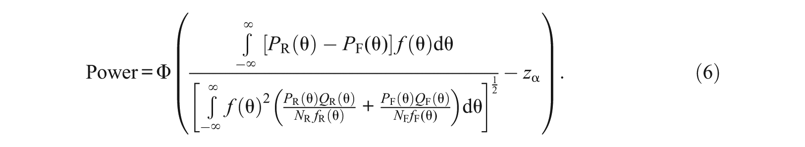
For now, consider the one-sided hypothesis testing problem of H 0 : β = 0 versus H 1 : β > 0 , where the null hypothesis is rejected if the SIBTEST statistic B is greater than a certain cutoff value c. By definition, the Type I error rate is the probability of rejecting the null, given that the null hypothesis is true: Type I error = P ( B > c | H 0 ) ; the power rate is the probability of rejecting the null, given that the alternative hypothesis is true: Power = P ( B > c | H 1 ) . Therefore, based on the asymptotic distribution for B under the null hypothesis,

Type I error = 1 − Φ ( c ) ,

where Φ ( c ) is the cumulative distribution function of the standard normal distribution. Let Type I error be fixed at α (e.g., α = .05). Solving for the cutoff value, we get c = z_α, where z_α is the (1 −α) quantile in the standard normal distribution, such that the tail area to its right is α (e.g., z_.05 = 1.645). Based on the asymptotic distribution for B under the alternative hypothesis,

Power = 1 − Φ ( z α − β σ ( β ^ ) ) = Φ ( β σ ( β ^ ) − z α ) .

Now substituting the values for β and σ ( β ^ ) as shown in Equations 1 and 2, we get

Power = Φ ( ∫ − ∞ ∞ [ E R ( Y | θ ) − E F ( Y |θ ) ] f ( θ ) dθ [ ∫ − ∞ ∞ f ( θ ) 2 ( σ R 2 ( Y | θ ) N R f R ( θ ) + σ F 2 ( Y | θ ) N F f F ( θ ) ) dθ ] 1 2 − z α ) .

Similarly, for the other one-sided hypothesis testing problem of H 0 : β = 0 versus H 1 : β < 0 , one rejects the null hypothesis if B > − z α , and the power formula is given by

Power = Φ ( − ∫ − ∞ ∞ [ E R ( Y | θ ) − E F ( Y |θ ) ] f ( θ ) dθ [ ∫ − ∞ ∞ f ( θ ) 2 ( σ R 2 ( Y | θ ) N R f R ( θ ) + σ F 2 ( Y | θ ) N F f F ( θ ) ) dθ ] 1 2 − z α ) .

For the two-sided hypothesis testing problem of H 0 : β = 0 versus H 1 : β ≠ 0 , one rejects the null hypothesis if | B | > z α / 2 , and the power formula is given by

Power = Φ ( ∫ − ∞ ∞ [ E R ( Y | θ ) − E F ( Y | θ ) ] f ( θ ) d θ [ ∫ − ∞ ∞ f ( θ ) 2 ( σ R 2 ( Y | θ ) N R f R ( θ ) + σ F 2 ( Y | θ ) N F f F ( θ ) ) d θ ] 1 2 − z α /2 ) + Φ ( − ∫ − ∞ ∞ [ E R ( Y | θ ) − E F ( Y | θ ) ] f ( θ ) d θ [ ∫ − ∞ ∞ f ( θ ) 2 ( σ R 2 ( Y | θ ) N R f R ( θ ) + σ F 2 ( Y | θ ) N F f F ( θ ) ) d θ ] 1 2 − z α /2 ) .

In the discussions that follow, we consider the power formula under the one-sided hypothesis testing H 0 : β = 0 versus H 1 : β > 0 , and the results can be easily extended to the other two testing problems.

Power Formula for SIBTEST With a Single Studied Dichotomous Item

SIBTEST was originally developed with the capability of testing the joint DIF effect of multiple studied items (differential bundle functioning [DBF]), and it was later extended to polytomous items (Chang, Mazzeo, & Roussos, 2005). The power formulas in Equations 3 5 are applicable for all the cases where SIBTEST can be applied: whether it is on a single studied item or a bundle of multiple items simultaneously and whether it is on dichotomous or polytomous items. We leave the discussions on the power of SIBTEST for DBF and polytomous items for future work. In this article, we focus on the case where DIF detection is conducted for each item one by one and the items are dichotomously scored, as this situation is most commonly found in practice. Also note that the power formulas in this article are only applicable for the SIBTEST procedures for unidirectional DIF, but not for the extended procedure for crossing DIF (CSIBTEST; Li & Stout, 1996).

In the situation where there is only one studied item and the studied item is dichotomous, E g ( Y | θ ) = P ( Y = 1 | θ , g ) = P g ( θ ) , g = R or F, where P g ( θ ) is the item response function (IRF) for group g; and σ g 2 ( Y | θ ) = Var ( Y | θ , g ) = P g ( θ ) Q g ( θ ) , where Q g ( θ ) = 1 − P g ( θ ) . By substituting these in Equation 3, we get the power formula for SIBTEST with a single studied dichotomous item:

Power = Φ ( ∫ − ∞ ∞ [ P R ( θ ) − P F ( θ ) ] f ( θ ) d θ [ ∫ − ∞ ∞ f ( θ ) 2 ( P R ( θ ) Q R ( θ ) N R f R ( θ ) + P F ( θ ) Q F ( θ ) N F f F ( θ ) ) d θ ] 1 2 − z α ) .

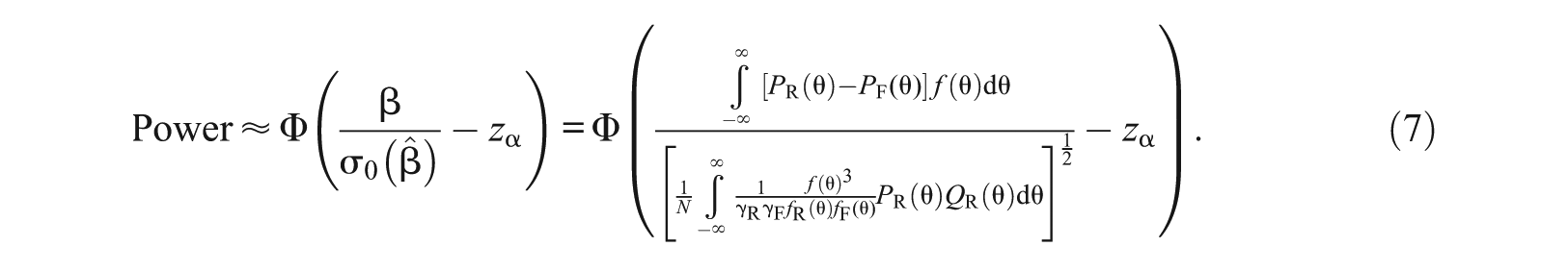
The Formula With Standard Error Evaluated Under Null Hypothesis

In the derivation of the power formula (Equation 6), the standard error σ ( β ^ ) as shown in Equation 2 is evaluated under the alternative hypothesis. It is possible to approximate σ ( β ^ ) with its value evaluated under the null hypothesis:

σ ( β ^ ) ≈ σ ( β ^ ) | H 0 = σ 0 ( β ^ ) = [ ∫ − ∞ ∞ f ( θ ) 2 ( 1 N R f R ( θ ) + 1 N F f F ( θ ) ) P R ( θ ) Q R ( θ ) dθ ] 1 2 = [ 1 N ∫ − ∞ ∞ 1 γ R γ F f ( θ ) 3 f R ( θ ) f F ( θ ) P R ( θ ) Q R ( θ ) d θ ] 1 2 ,

where γ R = N R / N , γ F = N F / N , and γ R + γ F = 1 . Using σ 0 ( β ^ ) in the place of σ ( β ^ ) in the power formula (Equation 6), we get

Power ≈ Φ ( β σ 0 ( β ^ ) − z α ) = Φ ( ∫ − ∞ ∞ [ P R ( θ ) − P F ( θ ) ] f ( θ ) dθ [ 1 N ∫ − ∞ ∞ 1 γ R γ F f ( θ ) 3 f R ( θ ) f F ( θ ) P R ( θ ) Q R ( θ ) dθ ] 1 2 − z α ) .

Using σ 0 ( β ^ ) in place of σ ( β ^ ) does not change the asymptotic behavior in large sample theory, and this technique is often used in the derivation of the power formula (e.g., see Lehmann, 1999, Theorem 3.3.3). Therefore, Equation 7 is still a valid power formula as is, of course, Equation 6.

In this case, one advantage of using σ 0 ( β ^ ) is that its integral (as shown in the denominator in Equation 7) does not involve the IRF for the focal group. In practice, this removes the burden of specifying P F ( θ ) . Very often, practitioners have no idea what P F ( θ ) is. Note that the numerator is simply the effect size β. That is, one may simply specify the desired effect size level to be detected.

A practitioner can ask the following question: What is the power of the SIBTEST to detect a DIF effect if the average difference in probability of getting correction response between the reference group and the focal group (i.e., β) is .10? To answer that question, one can use the standard error calculated under the null model, and the given β value to calculate the power.

Note in this formula, P R ( θ ) actually refers to “the IRF under the null hypothesis”; thus, it does not have to be the reference group IRF, sometimes it can also be the combined population IRF. One example is a DIF analysis on females versus males when the items are calibrated to the whole population. In this case, the whole population IRF can be used to evaluate the standard error under the null hypothesis.

Factors Influencing the Power of the SIBTEST

Based on the power formula (Equation 7), we can see that the power of SIBTEST is related to

It is obvious that an increase in power can be achieved in three ways: increasing the effect size β, decreasing standard error σ 0 ( β ^ ) , and getting smaller z α (i.e., larger Type I error α). For a given studied item, the item characteristic (IRF) is considered fixed and cannot be manipulated. Similarly, for the reference and focal populations, the distributions of the latent trait cannot be manipulated. The Type I error rate α is always a controlled value and usually fixed at .05. Therefore, in practice, once the studied item and reference and focal populations are determined, the only factors that can be manipulated are the sample size and the proportion of the focal group in the sample. One can always increase the sample size (including the total sample size or the sizes from either group) to reach the targeted power, and we defer the discussion on sample size calculation to a later section. When the total sample size N is fixed, a balanced design of γ F = γ R = .5 will have higher power than an unbalanced design. Therefore, in the situation where the total sample size has to be fixed due to limited resources, efforts to balance the group sizes, such as oversampling the smaller group (usually the focal group), will often increase the power.

For those factors that cannot be manipulated, the power formula can be used to understand how these factors influence the power. Note that in the power formula there is no specific requirement for the forms of the IRF and the latent trait distribution. In what follows, we discuss some of the most commonly used models, including the Rasch, 2PL, and 3PL models. Furthermore, we assume that the reference and focal group latent traits follow normal distributions.

Effect Size β Under IRT Models

The effect size β used by SIBTEST is a global measure of the DIF effect and can be seen as a weighted average of the local DIF effect [ P R ( θ ) − P F ( θ ) ] , where the weight is the density of the latent trait distribution in the population from which the reference and focal groups are sampled. For dichotomous items, it is the same as the standardized p-difference statistic by Dorans and Kulick (1986). A discussion on the relationship between β and other popular DIF effect size measures including the area between IRF (Raju, 1988), Mantel-Haenszel log-odds ratio (Holland & Thayer, 1988), and Delta-b (difference in difficulty) is provided in Appendix C in the online supplementary document.

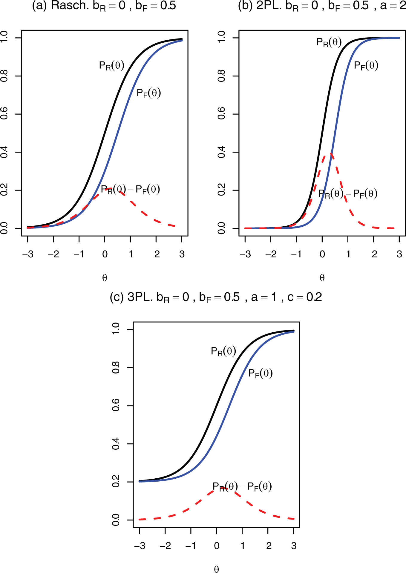
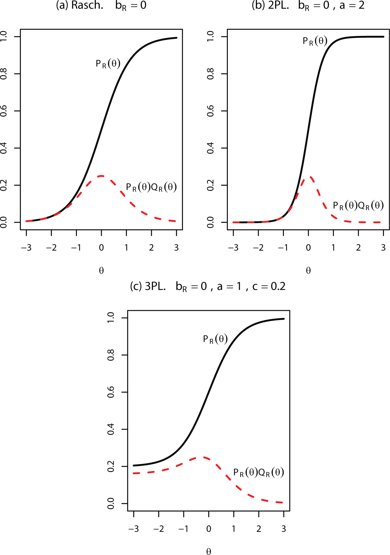
The IRF for the IRT 3PL model is given by

P ( θ ; a , b , c ) = c + ( 1 − c ) exp ( 1 . 7 a ( θ − b ) ) 1 + exp ( 1 . 7 a ( θ − b ) ) ,

where θ is the latent trait, a is the discrimination parameter, b is the difficulty parameter, and c is the guessing parameter. The IRF for the 2PL model is obtained by setting c = 0. And the IRF for the Rasch model is obtained by setting c = 0 and a = 1 / 1 . 7 .

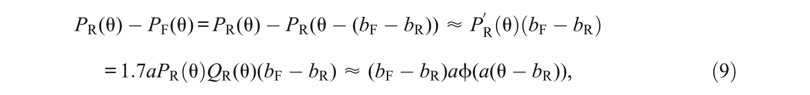
Figure 1 shows examples of the shape of the curve P R ( θ ) − P F ( θ ) under the Rasch, 2PL, and 3PL models. The curve under the Rasch or 2PL model has a bell shape that resembles a normal density curve. It turns out that a normal approximation does exist for P R ( θ ) − P F ( θ ) . Consider the 2PL models for P R ( θ ) and P F ( θ ) where a R = a F = a and b R ≠ b F , so that P F ( θ ) = P 2 PL ( θ ; a , b F ) = P 2 PL ( θ − ( b F − b R ) ; a , b R ) = P R ( θ − ( b F − b R ) ) . By Taylor expansion, we have the linear approximation

P R ( θ ) − P F ( θ ) = P R ( θ ) − P R ( θ − ( b F − b R ) ) ≈ P R ′ ( θ ) ( b F − b R ) = 1 . 7 a P R ( θ ) Q R ( θ ) ( b F − b R ) ≈ ( b F − b R ) a ϕ ( a ( θ − b R ) ) ,

OPEN IN VIEWER

Figure 1.

P R ( θ ) − P F ( θ ) under Rasch, 2PL, and 3PL models.

where the second approximation is based on the logistic-normal approximation (see Online Appendix A, Equation 21).

Now consider the effect size β when f ( θ ) is the density of the normal distribution with mean µ and standard deviation σ. By applying the normal approximation (Equation 9) and Equation 22 in Online Appendix B, the integral has a closed form approximation:

β = ∫ − ∞ ∞ [ P R ( θ ) − P F ( θ ) ] f ( θ ) dθ ≈ ( b F − b R ) ∫ − ∞ ∞ a ϕ ( a ( θ − b ) ) ( 1 σ ) φ ( θ − μ σ ) dθ = ( b F − b R ) 1 2 π( a − 2 + σ 2 ) exp ( − ( b R − μ) 2 2 ( a − 2 + σ 2 ) ) .

For the 3PL model with a R = a F = a , c R = c F = c , and b R ≠ b F , and f ( θ ) ~ N ( 0 , σ 2 ) , the effect size β has been shown (proof is given in Online Appendix B) to have a closed form approximate formula

β ≈ ( 1 − c ) ( b F − b R ) 1 2 π ( a − 2 + σ 2 ) exp ( − ( b R − μ ) 2 2 ( a − 2 + σ 2 ) ) .

From Equations 10 and 11, effect size β is the product of (1 −c), and the difference in difficulty Δ b = b F − b R , and the normal density function evaluated at b R , with mean µ and variance a − 2 + σ 2 . Effect size β is large when an item’s difficulty is close to the mean ability of the population; that is, | b R − μ | is small. It is hard to detect the DIF for an item that is too easy or too difficult relative to the target population because of the small effect size β.

How effect size β is influenced by a and σ is more complicated. Intuitively, a higher discrimination a will lead to a narrower shape for P R ( θ ) − P F ( θ ) , which may change the size of β in different ways depending on the difficulty of the item that determines the relative location between the P R ( θ ) − P F ( θ ) curve and the f ( θ ) curve. If the item difficulty is close to the mean ability, a higher a will lead to a higher effect size because of increased overlap between the two curves. However, if the item is too easy or too difficult, a higher a may lead to a lower effect size because of decreased overlap. Online Appendix D provides a detailed discussion based on Equation 11.

Standard Error σ 0 ( β ^ ) Under IRT Models

Beside the sample size N and the proportion γ F , other factors that influence the standard error are reflected in the integral

∫ − ∞ ∞ f ( θ ) 3 f R ( θ ) f F ( θ ) P R ( θ ) Q R ( θ ) dθ .

To simplify the discussion, let us consider the situation where the reference and focal groups have the same latent trait distribution and the integral becomes

∫ − ∞ ∞ P R ( θ ) Q R ( θ ) f ( θ ) d θ .

The integrand has two parts: P R ( θ ) Q R ( θ ) is related to the item characteristics and f ( θ ) is the latent trait distribution. Figure 2 shows the shape of the curve P R ( θ ) Q R ( θ ) under Rasch, 2PL, and 3PL models. For the Rasch or 2PL models, the curve has a symmetric bell shape peaked around b R , whereas for the 3PL model, it has an asymmetric bell shape. For the 2PL model, the derivative of the IRF P 2 PL ′ ( θ ) = 1 . 7 a P 2 PL ( θ ) Q 2 PL ( θ ) ; therefore, P R ( θ ) Q R ( θ ) has a bell shape as reflected by the logistic-normal approximation, and the area under the curve is ∫ − ∞ ∞ P R ( θ ) Q R ( θ ) dθ = [ P R ( ∞ ) − P R ( − ∞ ) ] / ( 1 . 7 a ) = 1 / ( 1 . 7 a ) .

OPEN IN VIEWER

Figure 2.

P R ( θ ) Q R ( θ ) under the Rasch, 2PL, and 3PL models.

Under the 2PL model with a common discrimination a and the assumption that f R ( θ ) = f F ( θ ) = f ( θ ) ~ N ( μ , σ 2 ) , by applying the logistic-normal approximation, we obtain the closed form solution in the same way Equation 10 was derived, resulting in

σ 0 ( β ^ ) = [ 1 N 1 γ R γ F ∫ − ∞ ∞ P R ( θ ) Q R ( θ ) f ( θ ) dθ ] 1 2 ≈ [ 1 1 . 7 aN γ R γ F 1 2 π ( a − 2 + σ 2 ) exp ( − ( b R − μ ) 2 2 ( a − 2 + σ 2 ) ) ] 1 2 .

Together with Equation 10, a closed form solution for the power formula under the 2PL model is

Power ≈ Φ ( β σ 0 ( β ^ ) − z α ) = Φ ( 1 . 7 a Nγ R γ F ( b F − b R ) [ 1 2 π( a − 2 + σ 2 ) exp ( − ( b R − μ) 2 2 ( a − 2 + σ 2 ) ) ] 1 2 − z α ) .

Note that if b R is fixed, Δ b = b F − b R is not related to the standard error σ 0 ( β ^ ) . When f ( θ ) is given, b R will influence the integral in a similar way to how it influences β: As b R gets farther away from the mean of f ( θ ) , the integral ∫ − ∞ ∞ P R ( θ ) Q R ( θ ) f ( θ ) dθ will become smaller, and, thus, the standard error will also get smaller. In this case, both β and σ 0 ( β ^ ) get smaller, but the ratio B = β / σ 0 ( β ^ ) gets smaller, because the numerator dominates the denominator with exponent 1 versus 1/2, as shown in the power formula Equation 13.

A larger discrimination parameter a tends to lead to a smaller standard error. However, as the behavior of the ratio B = β / σ 0 ( β ^ ) is dominated by the numerator β, the power is influenced by a in a similar fashion as β influenced by a.

For the 3PL model, as P 3 PL ( θ ) = c + ( 1 − c ) P 2 PL ( θ ) , it can be derived that P 3PL ( θ ) Q 3PL ( θ ) = c ( 1 − c ) Q 2PL ( θ ) + ( 1 − c ) 2 P 2PL ( θ ) Q 2PL ( θ ) . Compared with the 2PL model with the same parameters a and b , a non-zero guessing parameter c will lead to a larger standard error, and together with a smaller effect size, resulting in a smaller power for SIBTEST.

For the 3PL model with a R = a F = a and c R = c F = c , and assuming f ( θ ) ~ N ( μ , σ 2 ) , a closed form approximation for the standard error has been derived (Online Appendix B):

σ 0 ( β ^ ) ≈ [ 1 − c N γ R γ F { c Φ ( b R − μ a − 2 + σ 2 ) + ( 1 − c 1 . 7 a ) ( 1 2 π ( a − 2 + σ 2 ) ) exp ( − ( b R − μ ) 2 2 ( a − 2 + σ 2 ) ) } ] 1 2 .

Accordingly, the power formula is

Power ≈ Φ ( ( 1 − c ) ( b F − b R ) 1 2 π ( a − 2 + σ 2 ) exp ( − ( b R − μ ) 2 2 ( a − 2 + σ 2 ) ) [ 1 − c N γ R γ F { c Φ ( b R − μ a − 2 + σ 2 ) + ( 1 − c 1 . 7 a ) ( 1 2 π ( a − 2 + σ 2 ) ) exp ( − ( b R − μ ) 2 2 ( a − 2 + σ 2 ) ) } ] 1 2 − z α )

When f R ( θ ) and f F ( θ ) Differ

In previous discussion, we assumed that the reference and focal groups have the same latent trait distribution. If the two distributions differ, the DIF effect size β can be written as

β = ( 1 − γ F ) ∫ − ∞ ∞ [ P R ( θ ) − P F ( θ ) ] f R ( θ ) d θ + γ F ∫ − ∞ ∞ [ P R ( θ ) − P F ( θ ) ] f F ( θ ) d θ .

The effect size is large if the high value regions in both f R ( θ ) and f F ( θ ) overlap with the high value region in P R ( θ ) − P F ( θ ) , which is unlikely to happen as the difference between the mean of reference and focal distributions increases. Therefore, as the size of the difference in population means | d θ | = | μ F − μ R | increases, the power of SIBTEST tends to decrease.

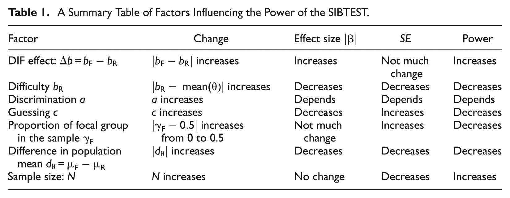
Table 1 summarizes what has been discussed so far. It lists the factors that may influence the power of SIBTEST, and how the change in each factor affects the DIF effect size, the standard error, and the power of SIBTEST. The situations we have discussed involve some typical factors in some typical setups. And we even derived some closed form formulas in these situations. However, the power formula (Equation 6 or 7) is very general, and its applicability should not be considered as only restricted to the situations we have discussed. For example, one situation we have not discussed is when the discrimination parameter in the 2PL or 3PL model has different values with regard to the reference and focal groups. Furthermore, there is no restriction that the IRF has to be 2PL or 3PL IRT models; it can be any form, for example, a normal ogive model, and so on. Also, the distribution of the latent trait may take forms other than the normal distribution.

OPEN IN VIEWER

Table 1.

A Summary Table of Factors Influencing the Power of the SIBTEST.

Factor	Change	Effect size | β |	SE	Power
DIF effect: Δ b = b F − b R	| b F − b R | increases	Increases	Not much change	Increases
Difficulty b R	| b R − mean( θ ) | increases	Decreases	Decreases	Decreases
Discrimination a	a increases	Depends	Depends	Depends
Guessing c	c increases	Decreases	Increases	Decreases
Proportion of focal group in the sample γ F	| γ F − 0 . 5 | increases from 0 to 0.5	Not much change	Increases	Decreases
Difference in population mean d θ = μ F − μ R	| d θ | increases	Decreases	Decreases	Decreases
Sample size: N	N increases	No change	Decreases	Increases

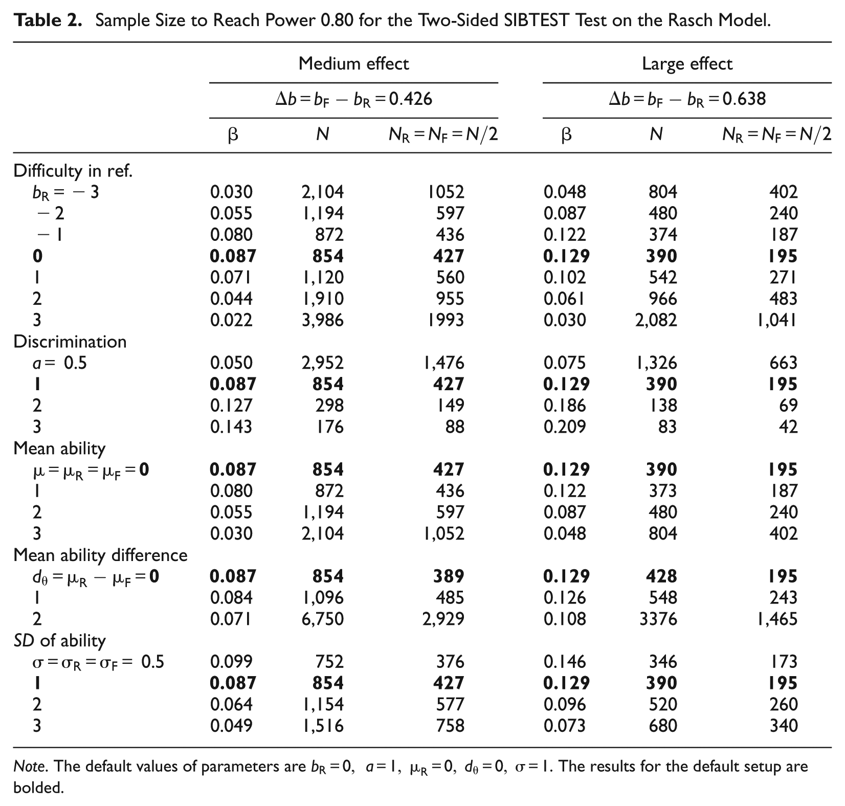
Sample Size Calculation

The most practical use of the power formula is probably the sample size calculation. Very often, one would like to calculate the minimal sample size N to achieve a certain power level (a well-accepted power value is 0.80). From the power formula, one can solve for N. For the one-sided test H 0 : β = 0 versus H 1 : β > 0 , the sample size formula is

N = ∫ − ∞ ∞ 1 γ R γ F f ( θ ) 3 f R ( θ ) f F ( θ ) P R ( θ ) Q R ( θ ) dθ [ ∫ − ∞ ∞ [ P R ( θ ) − P F ( θ ) ] f ( θ ) dθ ] 2 [ z 1 − power + z α ] 2 .

For the two-sided test, the power formula does not have a closed form solution for N, but one can find the solution using numerical methods such as trial and error or a binary search algorithm.

As an example, for the two-sided SIBTEST with a Type I error rate of 0.05, Table 2 shows the results of minimum sample size needed to achieve 0.80 power when the studied item follows the Rasch model. The default setup is that the reference difficulty b R for the studied item is 0; the latent trait distributions for both the focal and reference groups are N(0,1); and the group sizes are balanced ( N R = N F = N / 2 ) . We consider two values for Δ b = b F − b R : a medium effect value of Δ b = 0 . 426 and a large effect value of Δ b = 0 . 638 (Paek & Wilson, 2011; also see Appendix B in the supplementary document on why these two values were chosen). Under the default setup, the required sample size is 854 ( N R = N F = 427 ) for Δ b = 0 . 426 ; and the required sample size is 390 ( N R = N F = 195 ) for Δ b = 0 . 638 . The table shows sample sizes in the cases when one of the following factors changes while keeping the rest fixed at default values: the reference difficulty b_R, discrimination α, the mean ability µ, mean difference in ability d θ = μ R − μ F , SD of the ability σ. In each case, the effect size β is also reported. Note that the sample size is related not only to the effect size β but also to the standard error σ ( β ) ; therefore, different cases with similar β values may still have very different results for sample sizes.

OPEN IN VIEWER

Table 2.

Sample Size to Reach Power 0.80 for the Two-Sided SIBTEST Test on the Rasch Model.

	Medium effect			Large effect
	Δ b = b F − b R = 0 . 426			Δ b = b F − b R = 0 . 638
	β	N	N R = N F = N / 2	β	N	N R = N F = N / 2
Difficulty in ref.
b R = −3	0.030	2,104	1052	0.048	804	402
−2	0.055	1,194	597	0.087	480	240
−1	0.080	872	436	0.122	374	187
0	0.087	854	427	0.129	390	195
1	0.071	1,120	560	0.102	542	271
2	0.044	1,910	955	0.061	966	483
3	0.022	3,986	1993	0.030	2,082	1,041
Discrimination
a = 0.5	0.050	2,952	1,476	0.075	1,326	663
1	0.087	854	427	0.129	390	195
2	0.127	298	149	0.186	138	69
3	0.143	176	88	0.209	83	42
Mean ability
μ = μ R = μ F = 0	0.087	854	427	0.129	390	195
1	0.080	872	436	0.122	373	187
2	0.055	1,194	597	0.087	480	240
3	0.030	2,104	1,052	0.048	804	402
Mean ability difference
d θ = μ R − μ F = 0	0.087	854	389	0.129	428	195
1	0.084	1,096	485	0.126	548	243
2	0.071	6,750	2,929	0.108	3376	1,465
SD of ability
σ = σ R = σ F = 0.5	0.099	752	376	0.146	346	173
1	0.087	854	427	0.129	390	195
2	0.064	1,154	577	0.096	520	260
3	0.049	1,516	758	0.073	680	340

Note. The default values of parameters are b R = 0 , a = 1 , μ R = 0 , d θ = 0 , σ = 1 . The results for the default setup are bolded.

Monte Carlo Simulation Study

For simulation study, we adopted a design that is very similar to the simulation study conducted by Uttaro and Millsap (1994). Their simulation study looked at the factors that influence the detection of DIF by the Mantel-Haenszel procedure; while, in this article, we generate simulated data in a very similar design to study the behavior of SIBTEST, comparing the results with those predicted by the power formula. Each simulated data set is generated from the IRT 3PL model. Two test lengths are used: a short test with 20 items and a long test with 40 items. In a test form, only 1 item is the studied item, and the rest (19 or 39 items) are anchor items. For anchor items, the difficulty parameters were randomly picked from a N(0, 1) distribution; the discrimination parameters were randomly chosen from values 0.5, 1.0, and 1.5; and the guessing parameters were randomly chosen from values 0, 0.1, and 0.2. The same set of 19 or 39 anchor items were used in all the simulated test forms. For the single studied item, the item parameters for the reference group were a = 1 . 0 , b = 0 . 0 , and c = 0 . 2 . For the focal group item parameters and also the latent trait distributions, 36 conditions were considered by varying the following factors in a 3 × 3 × 2 × 2 factorial design with (a) three levels of discrimination parameter a: 0.5, 1.0, 1.5; (b) three levels of difficulty parameter b: 0.0, 0.3, 0.5; (c) two levels of guessing parameter c: 0.0, 0.2; and (d) two levels of differences in latent trait distribution means d θ : 0.0, −1.0. In each data set, 1,000 reference group examinees and 1,000 focal group examinees were sampled from the distributions θ R ~ N ( 0 , 1 ) , and θ F ~ N ( d θ , 1 ) , respectively. Each case was replicated 10,000 times. In the SIBTEST analysis, the total score of the 19 or 39 anchor items was used as the matching variable to stratify the examinees, and the SIBTEST procedure with a two-sided alternative hypothesis was conducted on studied items.

Table 3 summarizes the parameters used in the 36 cases, and the results for β, SE, B statistic, and the power for the simulated data sets. Under each quantity, three values were reported: the theoretical value as given by the formula presented in this article, the summary value from the SIBTEST results on the simulated data sets with 20 items, and the summary value for the 40-item data sets. The summary values for β and B are the mean of the corresponding estimates from 10,000 replicated data sets, the value for SE is the Monte Carlo SE, and the power is the observed rejection rate based on the p < .05 criterion. From the table, we observe that the theoretical values for β agree very well with the observed Monte Carlo mean values from both 20-item and 40-item simulation data. The root mean square difference between the theoretical value for β and the Monte Carlo mean of the β estimates is .0036 for 20-item tests, and .0046 for 40-item tests. The root mean square difference between the observed rejection rate and the theoretical power is 0.031 for 20-item tests, and 0.016 for 40-item tests. These results confirm that the power formula is accurate and is useful in estimating the power, even for short test forms. For SE, the theoretical values are very close to yet consistently slightly lower than the observed values (differences range from 0.002 to 0.005, about 5% to 10% of the SE value). Also note that the observed SE values for 40-item tests are very slightly yet consistently lower than those from 20-item tests (differences less than 0.002). One explanation for this is that the SE formula assumes a perfect match in θ when comparing the difference in response probability between the reference and focal groups, thus it ignores the small variability introduced by matching on the total score of the anchor items instead of matching on θ . This variability is larger for short tests than for longer tests. The power of the 36 cases ranges from 0.05 (the cases where there is no DIF) to near 1. Note that over the 36 cases, the SE values are actually similar: The values are all around 0.030, which means that the main driving force in the variability of the power over the cases is the differences in the effect size β.

OPEN IN VIEWER

Table 3.

Results From 36 Cases in the Simulation Study.

Simulation parameters					β			SE			Statistic B			Power
Case	a F	b F	c F	d θ	Theory	20-items	40-items	Theory	20-items	40-items	Theory	20-items	40-items	Theory	20-items	40-items
1	0.5	0	0	0	.10	.10	.10	0.028	0.030	0.030	3.53	3.40	3.40	0.94	0.92	0.92
2	0.5	0.3	0	0	.15	.15	.15	0.028	0.030	0.030	5.48	5.29	5.30	1.00	1.00	1.00
3	0.5	0.5	0	0	.19	.19	.19	0.028	0.030	0.029	6.78	6.56	6.56	1.00	1.00	1.00
4	0.5	0	0.2	0	.00	.00	.00	0.028	0.030	0.030	0.00	−0.02	0.00	0.05	0.05	0.05
5	0.5	0.3	0.2	0	.04	.04	.04	0.029	0.030	0.030	1.53	1.48	1.48	0.33	0.31	0.32
6	0.5	0.5	0.2	0	.07	.07	.07	0.029	0.030	0.030	2.52	2.44	2.45	0.71	0.68	0.68
7	1	0	0	0	.10	.10	.10	0.027	0.028	0.028	3.77	3.58	3.60	0.96	0.94	0.95
8	1	0.3	0	0	.18	.18	.18	0.026	0.028	0.028	6.97	6.67	6.71	1.00	1.00	1.00
9	1	0.5	0	0	.24	.24	.24	0.026	0.028	0.027	9.11	8.72	8.78	1.00	1.00	1.00
10 a	1	0	0.2	0	.00	.00	.00	0.027	0.029	0.028	0.00	0.00	−0.01	0.05	0.05	0.05
11	1	0.3	0.2	0	.07	.07	.07	0.028	0.029	0.029	2.43	2.34	2.36	0.68	0.64	0.65
12	1	0.5	0.2	0	.11	.11	.11	0.028	0.029	0.029	3.97	3.84	3.86	0.98	0.97	0.97
13	1.5	0	0	0	.10	.10	.10	0.025	0.028	0.027	3.98	3.73	3.78	0.98	0.96	0.96
14	1.5	0.3	0	0	.20	.20	.20	0.025	0.027	0.027	7.93	7.47	7.58	1.00	1.00	1.00
15	1.5	0.5	0	0	.26	.26	.26	0.025	0.027	0.026	10.54	9.94	10.10	1.00	1.00	1.00
16	1.5	0	0.2	0	.00	.00	.00	0.026	0.028	0.028	0.00	0.00	−0.01	0.05	0.05	0.05
17	1.5	0.3	0.2	0	.08	.08	.08	0.027	0.029	0.028	2.91	2.79	2.82	0.83	0.79	0.80
18	1.5	0.5	0.2	0	.13	.13	.13	0.027	0.029	0.028	4.72	4.55	4.58	1.00	1.00	0.99
19	0.5	0	0	−1	.08	.08	.08	0.033	0.037	0.035	2.53	2.27	2.39	0.71	0.61	0.66
20	0.5	0.3	0	−1	.14	.13	.13	0.034	0.037	0.035	4.04	3.85	3.93	0.98	0.96	0.97
21	0.5	0.5	0	−1	.17	.16	.17	0.034	0.037	0.035	5.01	4.88	4.93	1.00	1.00	1.00
22	0.5	0	0.2	−1	−.03	−.04	−.04	0.033	0.037	0.036	−0.99	−1.27	−1.11	0.17	0.27	0.21
23	0.5	0.3	0.2	−1	.01	.00	.00	0.034	0.037	0.036	0.22	−0.03	0.10	0.06	0.07	0.06
24	0.5	0.5	0.2	−1	.03	.03	.03	0.034	0.037	0.036	0.99	0.76	0.86	0.17	0.14	0.15
25	1	0	0	−1	.13	.12	.13	0.031	0.035	0.033	4.08	3.85	4.04	0.98	0.97	0.98
26	1	0.3	0	−1	.20	.20	.21	0.031	0.035	0.033	6.38	6.25	6.37	1.00	1.00	1.00
27	1	0.5	0	−1	.24	.24	.25	0.031	0.035	0.033	7.80	7.77	7.84	1.00	1.00	1.00
28 a	1	0	0.2	−1	.00	.00	.00	0.032	0.035	0.034	0.00	−0.16	0.03	0.05	0.08	0.06
29	1	0.3	0.2	−1	.06	.05	.06	0.032	0.036	0.035	1.79	1.65	1.80	0.43	0.39	0.44
30	1	0.5	0.2	−1	.09	.09	.10	0.033	0.036	0.035	2.85	2.74	2.86	0.81	0.77	0.81
31	1.5	0	0	−1	.14	.14	.15	0.029	0.034	0.032	4.94	4.69	4.92	1.00	1.00	1.00
32	1.5	0.3	0	−1	.22	.23	.24	0.029	0.034	0.032	7.65	7.47	7.63	1.00	1.00	1.00
33	1.5	0.5	0	−1	.27	.28	.28	0.029	0.034	0.032	9.29	9.20	9.30	1.00	1.00	1.00
34	1.5	0	0.2	−1	.01	.01	.02	0.030	0.035	0.033	0.47	0.35	0.56	0.08	0.08	0.09
35	1.5	0.3	0.2	−1	.08	.08	.09	0.031	0.035	0.034	2.52	2.43	2.59	0.71	0.67	0.74
36	1.5	0.5	0.2	−1	.12	.12	.13	0.032	0.036	0.034	3.70	3.62	3.76	0.96	0.94	0.96

Note. Item parameters for reference group: a R = 1 , b R = 0 , c R = 0.2. Sample Size: N R = 500 , N F = 500 . Latent trait distribution: θ R ~ N ( 0 , 1 ) , θ F ~ N ( d θ , 1 ) . Number of replicates in each case: 10,000. DIF = differential item functioning.

a

Cases with no DIF.

Discussion

In this article, we have derived a formula for calculating the power of the SIBTEST procedure for detecting DIF. The derivation is based on the asymptotic normal distribution of the SIBTEST test statistic, which assumes that the test length and the sample size are large. A comparison of the theoretical power from the formula and the observed rejection rate in the simulation studies has shown that the formula provides a close approximation to the true power and can thus be used in practical applications.

Several forms of the power formula for SIBTEST have been given in this article. For a dichotomous studied item, Equation 6 is a very general formula. In that formula, the IRFs, P R ( θ ) and P F ( θ ) can take either parametric or non-parametric forms, and so are the latent trait distributions, f R ( θ ) and f F ( θ ) . To conduct a power calculation, practitioners need to identify the models for the studied item and the distributions of the target populations, and have to make assumptions on some aspect of the item models. By using the standard error under the null hypothesis, the formula in Equation 7 releases practitioners from the burden of specifying the focal group IRF P F ( θ ) , which is usually unknown beforehand. And practitioners only need to specify the level of effect size β they care about.

In some cases, practitioners may still want to make assumptions on P R ( θ ) − P F ( θ ) , that is, how P F ( θ ) should be different from P R ( θ ) . Does P F ( θ ) have the same type of IRT model as in the reference IRT model? If both P R ( θ ) and P F ( θ ) follow IRT 3PL model, shall we assume a F = a R ? Shall we assume c F = c R ? What values of Δ b = b R − b F to choose? The simulation study is a vivid example of the ramification of different choices of model for P F ( θ ) , while P R ( θ ) is the same, the different choices for P F ( θ ) in the 36 cases produce different power values. The good news is that the power formula can be applied to all these cases. Practitioners have to make decisions on what assumptions look reasonable or are of interest to their problem. For example, it is often reasonable to assume that a F = a R and c F = c R , and focus on the power calculation on different choices of b R − b F . In this case, the closed form formulas in Equations 13 and 15 can be used.

The formulas for power and sample size calculation presented in this article have been implemented in an R package that is available to public at the author’s website.