
Abstract
Marginal maximum likelihood estimation based on the expectation–maximization algorithm (MML/EM) is developed for the one-parameter logistic model with ability-based guessing (1PL-AG) item response theory (IRT) model. The use of the MML/EM estimator is cross-validated with estimates from NLMIXED procedure (PROC NLMIXED) in Statistical Analysis System. Numerical data are provided for comparisons of results from MML/EM and PROC NLMIXED.
Introduction
Psychological constructs are hypothetical concepts that cannot be observed directly, but theorized to explain human behavior. Examples include intelligence, motivation, self-esteem, mathematics proficiency, and happiness. Although these constructs cannot be observed directly, their existence can be inferred through various behaviors. For example, mathematics proficiency can be inferred by observing a person’s responses to an instrument (i.e., a mathematics test). By placing an individual on this latent continuum, measuring the construct is formally established. As one of the tools for measuring constructs, item response theory (IRT) models how the trait level is related with an individual’s response to an item. In applying this to education, trait levels are realized as latent variables (theta, trait continuum, or scale), which represent the individual’s ability within a specific knowledge domain. Furthermore, one or more item parameters characterize an individual item. Assuming success or failure on an item follows independent Bernoulli distribution, the Rasch model (Lord & Novick, 1968) relates the probability of pass/fail on item with the difference between person ability and item difficulty through the logistic link function.
In terms of IRT modeling, multiple-choice (MC) items impose an interesting problem that cannot be handled with the conventional Rasch model: guessing. There are diverse parameterizations and interpretations used to accommodate the guessing behavior. As a result, various IRT models have been proposed to explain guessing behavior within the model: (a) a fixed value of
1PL-AG
One of the interpretations of the 3PL model is that item responses are composed of two processes: a p-process and a g-process (Hutchinson, 1991). The p-process is an item-solving process, whereas the g-process is a guessing process. One possible arrangement of executing the two processes is that the g-process is followed by the p-process: An examinee attempts to solve an item and resorts to guessing only if a correct response is not identified. While applying this process model, 1PL-AG was motivated from the observation that the success of guessing depends on ability. For instance, an examinee with higher ability may have a higher chance of success on the g-process, perhaps, due to his or her greater ability to recall relevant facts and connect separate knowledge to make a correct choice. According to the 1PL-AG, the probability of passing an item j given ability θ i and item parameters is
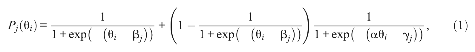
where
As α is a positive value, the probability of passing an item due to the g-process increases as the ability increases. However, as the g-process is weighted by the probability of the failed p-process (i.e., 1 − p-process), which approaches zero as ability increases, the net contribution of the g-process decreases at high ability. In addition, as the g-process approaches zero as ability decreases, the net contribution of guessing deceases at low ability. According to San Martín et al. (2006), the interpretation for the low contribution from the g-process at both extremes is that low-ability examinees are attracted by the distractors and not able to find the correct answer, whereas high-ability examinees do not necessarily resort to guessing to choose the correct response.
Recently, researchers have raised model identification issue related with 1PL-AG (Maris & Bechger, 2009; San Martín, Rolin, & Castro, 2013). Model identifiability states that there is a one-to-one relationship between the parameters and the sampling distributions. Under the sampling theory framework, it is not possible to obtain unbiased and/or consistent estimators of parameters if identifiability does not hold (Gabrielsen, 1978; Koopmans & Reiersol, 1950). Maris and Bechger (2009) have shown that 3PL is not identifiable if all discrimination is held to a constant value (i.e., called 1PL-G). For example, it can be shown in 1PL-G that parameter values of (θ, difficulty, guessing) of both (2.0, 1.2, 0.2) and (2.0134428, 1.1694177, 0.1751562) result in same probability of passing an item, 0.7519796. Then, it cannot be determined which set of parameter should be used for the correct inference. This identification issue is relevant to the current study because 1PL-G is nested within 1PL-AG by setting α to zero.
The model identifiability problem, however, should be considered under the context of the sampling distribution and the parameter of interest (San Martín et al., 2013). For instance, the identification problem differs significantly depending on whether the abilities are specified as fixed effects versus random effects. For fixed-effects specification, the parameters of interest during the estimation include θ, whereas the random-effects specification marginalizes the likelihood function and θ is integrated out using a known (or partially known) ability distribution. It is known that 1PL-G could be identified by fixing one guessing parameter to a known value (e.g., zero for convenience) under the random-effects specification and that the ability distribution is known up to the scale parameter (San Martín et al., 2013). Whether this issue imposes any practical limitation for 3PL or 1PL-AG model is still an open question. Furthermore, question on whether the identification problem still remains when the ability distribution is fully specified (i.e., location and scale are assumed to be known) has not answered yet.
In terms of parameter estimation, PROC NLMIXED has been the primary estimation tool because of programming ease. However, the 1PL-AG model has been vastly underused due to, we believe, the lengthy estimation time. Therefore, the current study develops and evaluates an efficient estimator based on the marginal maximum likelihood estimation with the expectation–maximization algorithm (MML/EM) for the 1PL-AG model (Bock & Aitkin, 1981). The rest of the article is organized as follows. Estimation methodologies under the IRT framework are introduced and the MML/EM for the 1PL-AG model is derived. A simulation study and its results are presented, followed by the discussion.
Method
MML/EM Estimation Algorithm for the 1PL-AG Model
The conditional probability for an examinee i to respond in pattern
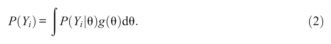
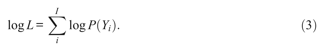
Under the assumption of independence of observations, the logarithmic transformation of the probability of response patterns for I randomly chosen examinees becomes
The derivation of the marginal likelihood equations begins with the first derivatives with respect to a parameter ζ:
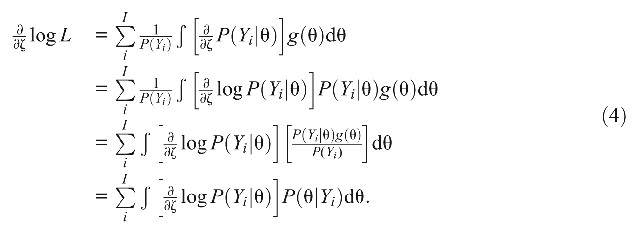
Furthermore, the first derivative of the conditional likelihood function is expressed as
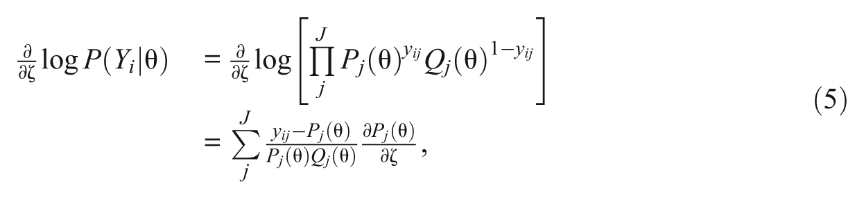
where yij is the dichotomous response to item j of examinee i; Pj (θ) is the probability of being correct on item j for an examinee of ability θ; and Qj (θ) is 1 −Pj (θ).
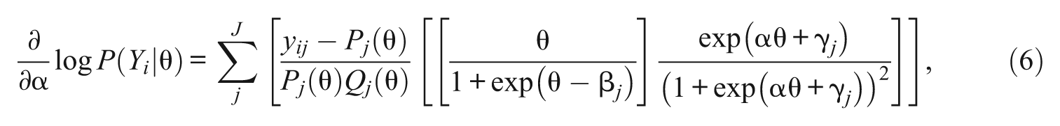
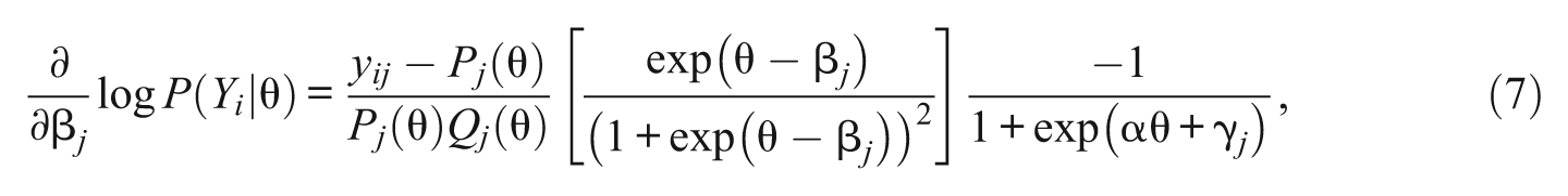
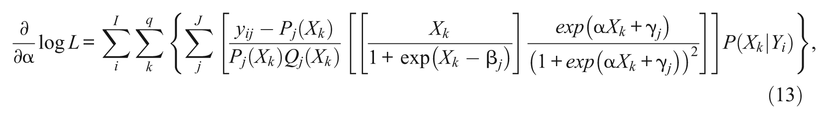
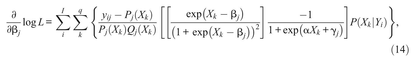
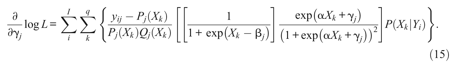
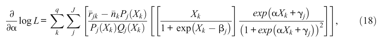
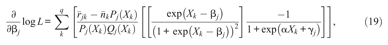
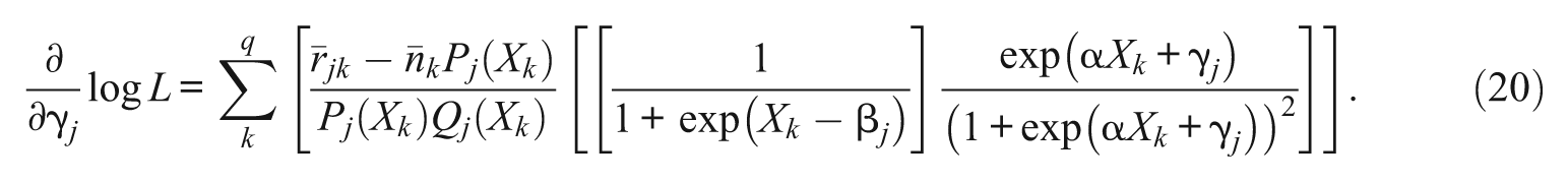
For each of 1PL-AG parameters, α, β j , and γ j , the first derivatives of the conditional likelihood functions are
and
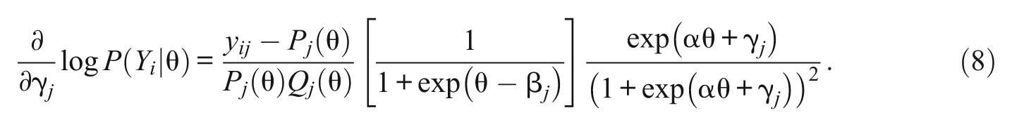
Note that except for the parameter α, which is common across items, the first derivatives of β j and γ j do not depend on β h , and γ h of j≠h. Plugging Equations 6, 7, and 8 into 4, the marginal likelihood equations for α, β j , and γ j are
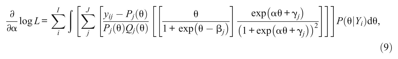
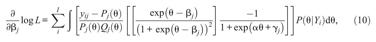
and
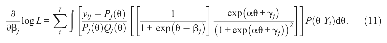
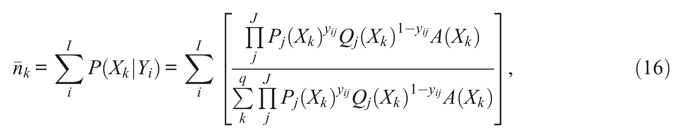
Equations 9, 10, and 11 represent a nonlinear system of equations that need to be solved for their roots. The integral within the equations can be accomplished through numerical integration, which is the approximation of integrating a continuous curve through the summation of a rectangular area. The integrands, the functions under integration, are evaluated at a finite set of points called “integration points” (or quadrature points). The prior ability distribution, g(θ), is approximated by taking a finite number of quadrature points, Xk
for
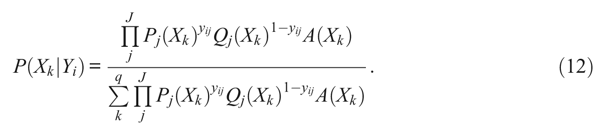
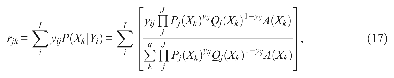
This equation limits the continuous distribution of the posterior ability of examinee i, θ i , into a finite number of quadrature points. Assuming a unit normal distribution of θ, quadrature points and their weights can be obtained from Gaussian quadrature formula (Stroud & Secrest, 1966). In addition, values of A(Xk ) could be adjusted at each iteration by empirically estimated weights (Mislevy, 1984). As suggested from Equation 12, however, the impact of the prior ability distribution is insignificant with a practically large number of items (Bock & Aitkin, 1981). Intuitively, the ability distribution of a sample conditional on the observation of responses to items depends mainly on the item responses and their characteristics rather than on the population ability distribution, if responses are drawn from enough items. The marginal likelihood equations using Equation 12 are
and
Equations 13, 14, and 15 are marginal likelihood functions of the parameters of the entire set of J items through the posterior ability distribution, P(Xk
|Yi
). Therefore, (2J+ 1) marginal likelihood equations should be solved simultaneously. However, solving entire equations imposes an intractable computational burden of generating and inverting a (2
Bock and Aitkin (1981) applied the EM algorithm to transform a regular MML estimation to a missing data problem. For that, two artificial quantities are introduced:
and
where
and
To summarize, the complete steps for MML/EM algorithm are as follows:
E-step: Given the response strings, the provisional initial parameters, and the quadrature weight A(Xk
), compute the expected number of examinees on each Xk
,
M-step: For each item, find the roots for Equations 18, 19, and 20 via a numerical method such as the Newton–Raphson method.
The MML/EM algorithm is an iterative process such that the E-step and M-step are repeated until item parameters satisfy the predefined convergence criterion. A careful examination should reveal that Equations 19 and 20 for an item j do not depend on the parameters of an item h, where j≠h, because
Simulation Study
The main goals of this simulation study are twofold. First, the recovery of 1PL-AG model parameters is examined using the MML/EM method presented previously. For this, the following steps are taken: (a) Implement MML/EM for the 1PL-AG in Java language; (b) generate response strings of three groups of examinees (i.e., 2,500, 3,000, and 3,500) to 20 1PL-AG items of α = (0.065, 0.265, 0.365) and βs and γs from true values in Table 1. βs are difficulty parameter and γs are guessing at θ = 0 in logistic scale. Mean, standard deviation, minimum and maximum for βs and γs are (0.641, 1.021, −1.3697, 2.097) and (−1.223, 0.644, −2.502, −0.23), respectively, and 20 values are randomly sampled within the ranges. The generated true parameter values in the current study are guided by the work from San Martín et al. (2006). (c) Perform parameter estimations for 3 (αs) × 3 (sample sizes) conditions. (d) Repeat Steps (b) and (c) 50 times and examine the performance of parameter recoveries in terms of their root mean square errors (RMSEs) and standard errors. The differences between true and estimated parameters are squared and averaged over 50 replications. Then squared root is taken for each βs, α, and γs. Empirical standard errors for each parameter estimates were derived based on 50 replications as well.
Recovered Estimates From MML/EM.

Note. MML = marginal maximum likelihood; EM = expectation–maximization algorithm.
Second, the performance comparison between MML/EM and PROC NLMIXED is made in terms of biases and estimation times. For this, 50 replications of parameter recoveries are performed with PROC NLMIXED for the same 3 × 3 conditions. The same number of Gauss–Hermite quadrature points (i.e., 10 points) and the same convergence criterion (i.e., The difference of −2 × Log-likelihood (−2 ×l) values between two successive EM iterations being smaller than 10E-3) are applied for both MML/EM and PROC NLMIXED. The results from both the MML/EM and PROC NLMIXED procedures are compared based on estimation accuracy and simulation time. RMSEs are used for evaluating estimation accuracy for each items. For example, RMSE for β j is
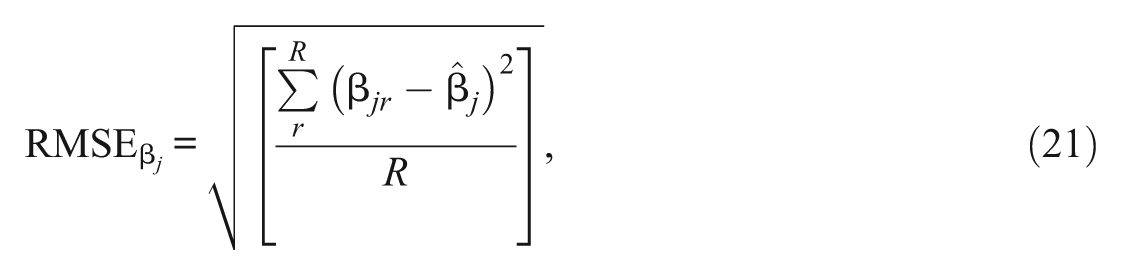
where R is the number of replications (i.e., 50), β
jr
is the estimated parameter for item j in rth replication, and
The simulation time for MML/EM was measured after the initial values for convergence of the Newton–Raphson method were obtained. SAS version 9.3 was used, and the simulations were performed using a computer with the following specifications: AMD Phenom II X4 CPU, 3.4 GHz, 512 KB Cache, and 6 GB of RAM.
Results
Tables 1 and 2 present parameter recoveries for individual items (in the order of βs, α, and γs) in each condition.
Recovered Estimates From PROC NLMIXED.

Tables 3 and 4 present of RMSEs for individual items (in the order of βs, α, and γs) in each condition.
RMSE for the Estimates From MML/EM.
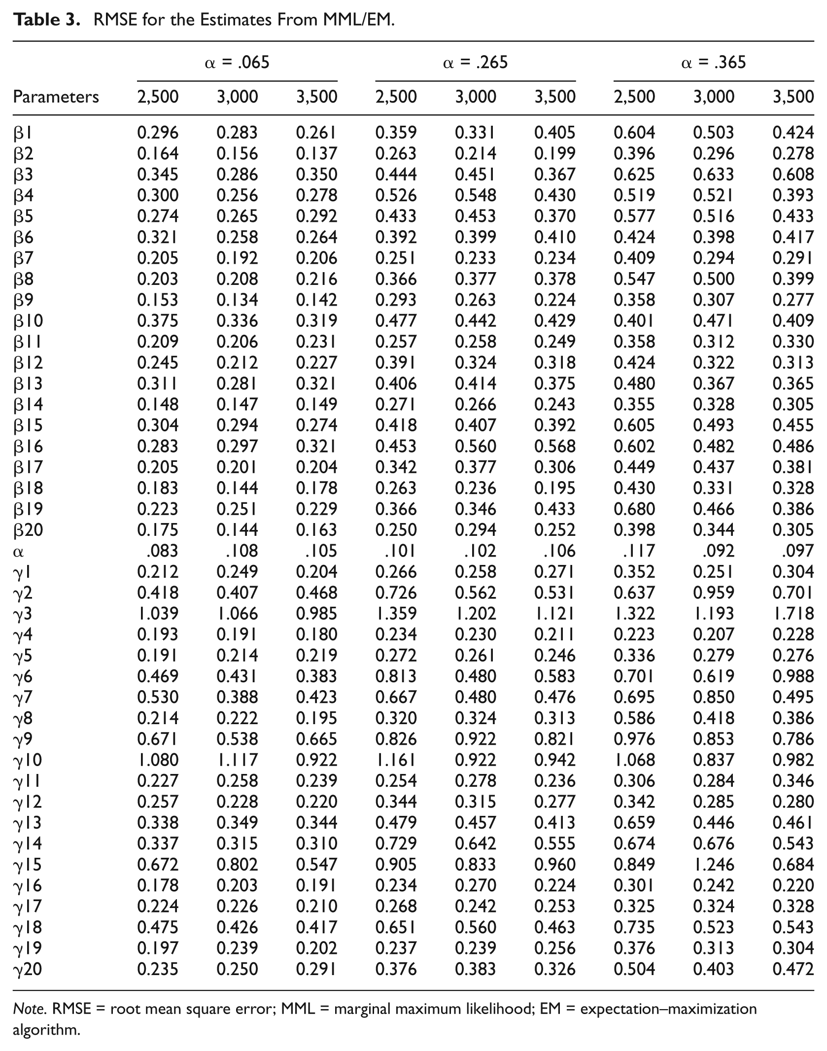
Note. RMSE = root mean square error; MML = marginal maximum likelihood; EM = expectation–maximization algorithm.
RMSE for the Estimates From PROC NLMIXED.
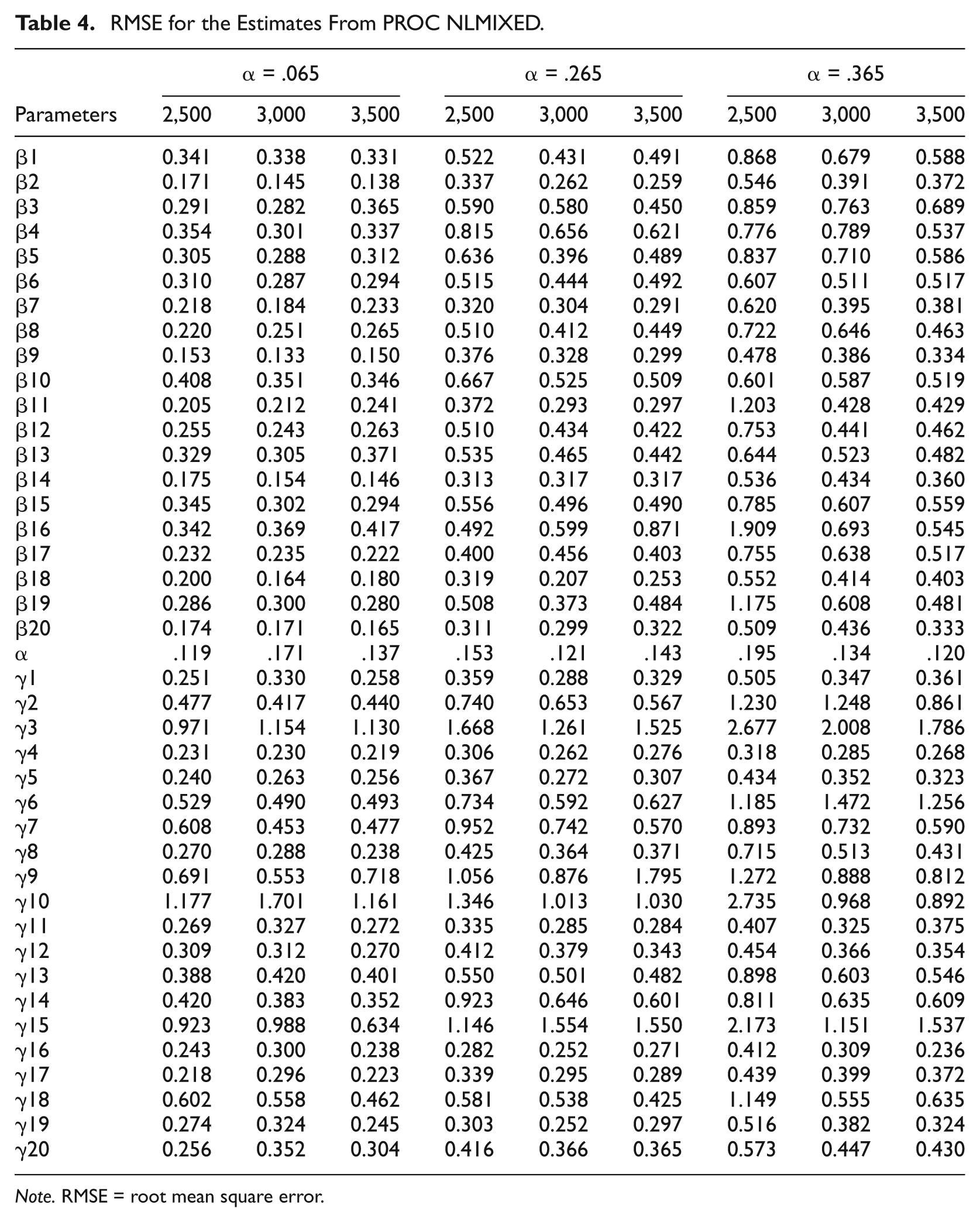
Note. RMSE = root mean square error.
Table 5 shows empirical standard errors. In addition, standard errors from MML/EM and PROC NLMIXED were analytically estimated, and the ratios of the average estimated standard errors to the empirical standard errors were presented within the parentheses. The values close to ones indicate that estimated standard errors are accurate to the empirical standard errors. MML/EM resulted in smaller standard errors for αs, whereas PROC NLMIXED produced smaller standard errors for βs. Standard errors for γs were comparable for both methods. As shown in Table 5, the standard errors decreased as the sample sizes increased. Large standard error values for γs imply large variations for estimates of guessing parameter.
Average Empirical Standard Error of Estimates for MML/EM and PROC NLMIXED.
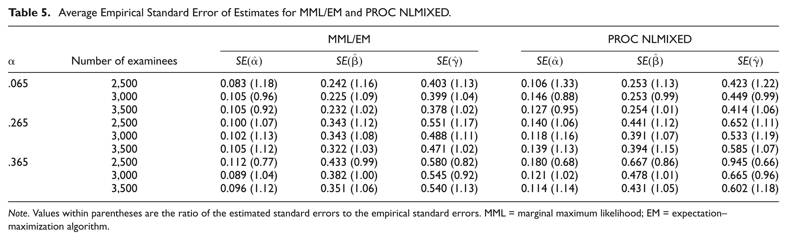
Note. Values within parentheses are the ratio of the estimated standard errors to the empirical standard errors. MML = marginal maximum likelihood; EM = expectation–maximization algorithm.
Table 6 presents simulation time and a model fit statistic (i.e., −2 ×l) for each of the estimation methods. For PROC NLMIXED, the simulation took from 1.85 to 3.72 hr, whereas MML/EM took from 15.5 to 50 s. There is a clear pattern of increased estimation time as sample size increases. PROC NLMIXED and MML/EM methods both showed the largest simulation time for α = .265. In terms of the −2 ×l, the differences between the MML/EM and PROC NLMIXED were small, demonstrating that both procedures produced similar values in terms of their likelihoods.
Simulation Time and Fit Statistics for MML and PROC NLMIXED.
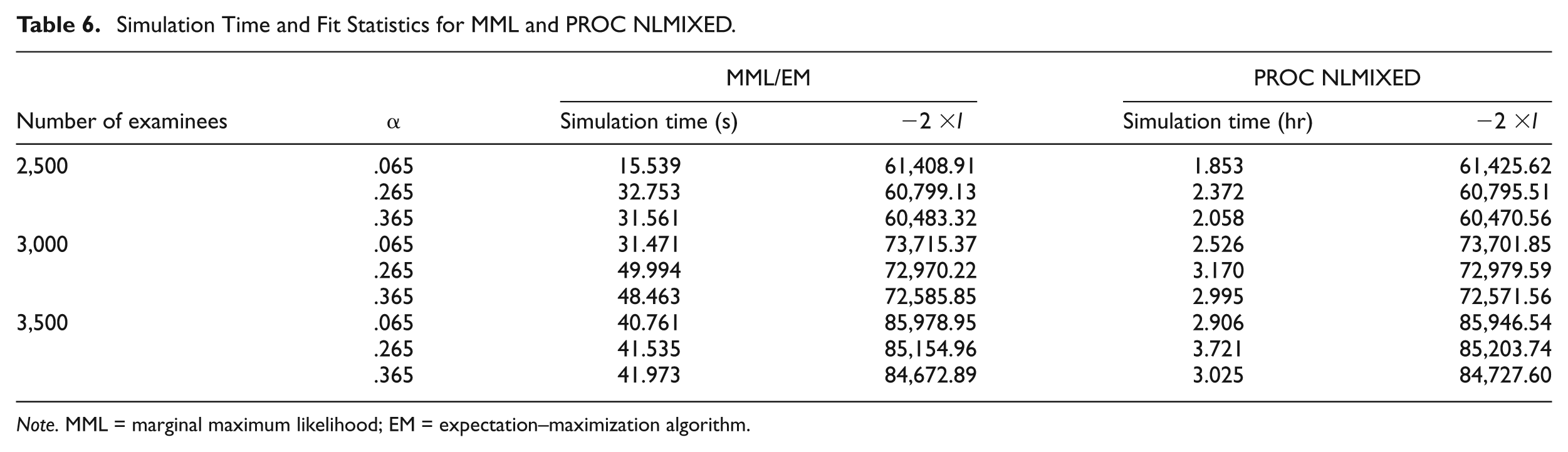
Note. MML = marginal maximum likelihood; EM = expectation–maximization algorithm.
Discussion
The advancement of the IRT model has been intertwined with the development of parameter estimation techniques. Recent attention on the IRT model as examples of the NLMIXED model expanded the understanding and interpretation of parameters in IRT models. The relationship between two somewhat distinct models already was predicted by Bock and Lieberman (1970), when they regarded abilities as random effects. Methods of NLMIXED and MML/EM take a common approach: the maximization of the marginalized likelihood function. While widely available NLMIXED estimators perform direct optimization after marginalization (Rijmen, Tuerlinckx, De Boeck, & Kuppens, 2003), MML/EM incorporates estimations of the distributions of ability parameters. Through this augmentation of person parameter information for item parameter estimation, MML/EM achieves a faster convergence.
Most of the research on the 1PL-AG model has been based on the use of PROC NLMIXED for the parameter estimation. Although it provides ease of programming, lengthy estimation time associated with PROC NLMIXED encouraged an alternative estimation procedure. The main contribution of the current study, we believe, is the development of a more efficient estimation procedure for the 1PL-AG model. For the demonstration of the MML/EM method, a simulation study was conducted and compared with the current standard estimation procedure. The results indicated that MML/EM method produced estimates that were comparable with the PROC NLMIXED in a fraction of the time. As the performance of the PROC NLMIXED procedure has not, to our knowledge, been compared with other estimation methods, this study supports the general accuracy of this procedure as well.
The conceptualization and interpretation of guessing in educational testing settings are far from being settled. There is not a single model that fully explains underlying interactions between ability and item characteristics occurring from guessing. Even the most popular model, the 3PL, explains the probability of guessing for low-ability examinees, whereas the 1PL-AG focuses on guessing behavior for mid-ability examinees. For the 1PL-AG, guessing is the secondary or auxiliary problem-solving process conditional on the failure of the main process used to respond to an item. Therefore, low-ability examinees lack this ability, whereas high-ability examinees do not have to depend on it.
Modeling factors that influence examinee’s responses with IRT models is an ongoing effort. Therefore, further research should follow. First, a possible instability between the discrimination and the guessing parameter in the 3PL (van der Linden & Hambleton, 1997) may be applicable to 1PL-AG model. Second, the application of EM for NLMIXED reported by Walker (1996) opens interesting comparison study with MML/EM method. Third, a more systematic approach for obtaining initial values of MML/EM will accelerate wide adoption of MML/EM estimation. As each Newton–Raphson process takes less than a minute for conditions in this study, even with an elaborate search method, MML/EM should still hold a substantial advantage in terms of computing time compared with other methods. Fourth, there has been several studies compared the performance between Markov chain Monte Carlo (MCMC) and MML estimation for binary outcomes (Albert, 1992; Baker, 1998; Kieftenbeld & Natesan, 2012; Kim, 2001). However, to our knowledge, no studies have been done comparing the performance between MCMC and NLMIXED. Therefore, future study comparing the performance between MCMC and SAS PROC NLMIXED for 1PL-AG will provide useful information for the choice of estimation method. Last, two-parameter logistic model with ability-based guessing (2PL-AG) should be investigated at as a natural extension of 1PL-AG. 2PL-AG conceptualizes the discriminating power of each item by allowing discrimination parameters to be freely estimated, while also including ability-based guessing process. However, another interesting approach is to view 2PL-AG as a 3PL model with ability-based guessing. Unlike the constant probability of guessing in 3PL, a monotonic increasing probability of success of guessing on the ability scale can be modeled in 2PL-AG. When α (i.e., the weight on ability in the guessing process) is fixed to zero, 2PL-AG is reduced to 3PL, which makes 3PL a nested model of 2PL-AG. The difference in the number of item parameters between two models is only one. It is believed that a model comparison among 2PL-AG, 3PL, and 1PL-AG would be worth further investigation.
Footnotes
Declaration of Conflicting Interests
The author(s) declared no potential conflicts of interest with respect to the research, authorship, and/or publication of this article.
Funding
The author(s) received no financial support for the research, authorship, and/or publication of this article.