



Abstract
Over the last decade, researchers have come to recognize the benefits of ideal point item response theory (IRT) models for noncognitive measurement. Although most applied studies have utilized the Generalized Graded Unfolding Model (GGUM), many others have been developed. Most notably, David Andrich and colleagues published a series of papers comparing dominance and ideal point measurement perspectives, and they proposed ideal point models for dichotomous and polytomous single-stimulus responses, known as the Hyperbolic Cosine Model (HCM) and the General Hyperbolic Cosine Model (GHCM), respectively. These models have item response functions resembling the GGUM and its more constrained forms, but they are mathematically simpler. Despite the apparent impact of Andrich’s work on ensuing investigations, the HCM and GHCM have been largely overlooked by applied researchers. This may stem from questions about the compatibility of the parameter metric with other ideal point estimation and model-data fit software or seemingly unrealistic parameter estimates sometimes produced by the original joint maximum likelihood (JML) estimation software. Given the growing list of ideal point applications and variations in sample and scale characteristics, the authors believe these HCMs warrant renewed consideration. To address this need and overcome potential JML estimation difficulties, this study developed a marginal maximum likelihood (MML) estimation algorithm for the GHCM and explored parameter estimation requirements in a Monte Carlo study manipulating sample size, scale length, and data types. The authors found a sample size of 400 was adequate for parameter estimation and, in accordance with GGUM studies, estimation was superior in polytomous conditions.
Over the last decade, researchers have come to recognize the benefits of ideal point item response theory (IRT) models for noncognitive scale construction and scoring. Ideal point models have been applied in areas such as attitude (e.g., Andrich, 1988, 1989; Andrich & Styles, 1998; Roberts & Laughlin, 1996), health (Andrich & Van Schoubroeck, 1989), personality (Carter et al., 2014; Chernyshenko, Stark, Chan, Drasgow, & Williams, 2001; Stark, Chernyshenko, Drasgow, & Williams, 2006), vocational interest (Tay, Ali, Drasgow, & Williams, 2011), job satisfaction (Carter & Dalal, 2010), and performance (Borman et al., 2001) measurement.
To date, the vast majority of applied studies have utilized the Generalized Graded Unfolding Model (GGUM; Roberts, Donoghue, & Laughlin, 2000), even though many other ideal point models have been developed. Most notably, David Andrich and colleagues published a series of papers comparing dominance and ideal point measurement perspectives (Andrich, 1978, 1995, 1996), and they proposed ideal point models for dichotomous and polytomous single-stimulus responses, known as the Hyperbolic Cosine Model (HCM; Andrich & Luo, 1993) and the General Hyperbolic Cosine Model (GHCM; Andrich, 1996), respectively. These models have item response functions (IRFs) resembling the GGUM and its submodels, particularly the “partial credit model” which constrains discrimination parameters to 1 (Roberts & Laughlin, 1996), yet the GHCM probability equation is somewhat simpler, making it easier to compute derivatives analytically for parameter estimation and generalize the model for multidimensional forced-choice (MFC) applications (e.g., Seybert, 2013).
Despite the apparent impact of Andrich’s work on ensuing model development (e.g., Roberts et al., 2000; Stark, Chernyshenko, & Drasgow, 2005), model-data fit (Chernyshenko et al., 2001; Stark et al., 2006), and scale construction (Chernyshenko, Stark, Drasgow, & Roberts, 2007; Roberts, Laughlin, & Wedell, 1999) investigations, the HCM and GHCM have been largely overlooked by applied researchers. This may be due to questions about the compatibility of the parameter metric with other ideal point estimation and model-data fit software or concerns about some seemingly unrealistic parameter estimates produced by the early joint maximum likelihood (JML) estimation software (e.g., location parameter estimates well beyond the −3 to +3 range observed with most models; Stark, Chernyshenko, Lee, & Drasgow, 2000).
Given the growing list of ideal point applications and the variations in sample and scale characteristics in applied research, the authors believe that these HCMs warrant renewed consideration. To address this need and avoid potential difficulties with JML estimation, this study developed a new marginal maximum likelihood expectation-maximization (MML-EM) algorithm for the GHCM and explored parameter estimation requirements in a Monte Carlo study manipulating sample size, scale length, and data types. To illustrate the properties of this model, this study shows GHCM IRFs and item information functions (IIFs), and use the MML-EM algorithm to calibrate responses to a 20-item Orderliness scale (Chernyshenko, 2002).
The General Hyperbolic Cosine Model (GHCM)
Andrich (1996) proposed the GHCM for ordered categorical responses. It is an extension of the earlier HCM for dichotomous data. The probability function for the GHCM is


where

Note that
Figure 1 presents illustrative GHCM category response functions (CRFs) and IRFs (i.e., expected value functions) for two four-option polytomous items. Panels (a) and (b) present the CRFs and IRF for the first item, and Panels (c) and (d) present the CRFs and IRFs for the second item. Note that the CRFs are symmetric around the item location parameters (

Illustrative GHCM category response functions and item response functions.
Item Information
Previous studies have derived item information for the GHCM using Samejima’s (1969) definition of information for polytomous IRT models (e.g., Luo, 2001; Luo & Andrich, 2005). Let

where Fisher information

By substitution, item information can be rewritten as

where


where


Figure 2 presents GHCM IIFs for the two- and four-option items, respectively. Consistent with IIFs of the GGUM, the GHCM IIFs are bimodal and symmetric, and item information is zero at |
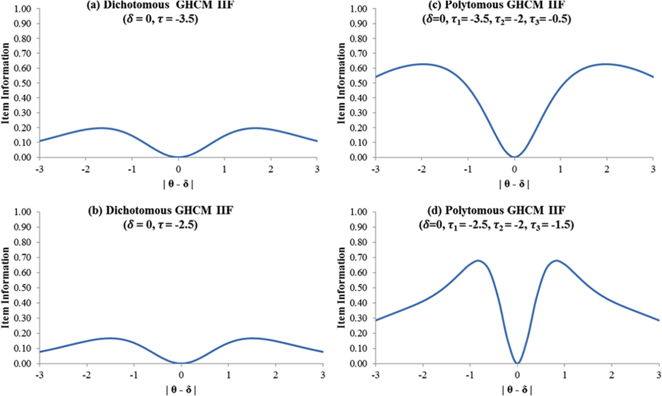
Illustrative GHCM item information functions.
Item Parameter Estimation
An advantage of MML estimation over JML estimation is that the MML parameter estimates are consistent. The number of parameters to estimate does not increase as sample size increases because person parameters are integrated out of the likelihood function. In this research, MML estimation of GHCM item parameters was accomplished using an expectation-maximization (EM) algorithm (Bock & Aitkin, 1981; Robert et al., 2000). The necessary equations for the GHCM were derived as follows.
Let

and

For examinees randomly sampled from a population with trait distribution

Let N represent the total number of response patterns (i.e., examinees), S represent the number of unique response patterns (s = 1, 2, …, S), and

and the marginal log likelihood is

To estimate GHCM item parameters, the partial derivatives of Equation 12 with respect to

Furthermore,

For a specific item j, because partial derivatives with respect to

Similarly, the derivative of the marginal likelihood with respect to

The integrations in these equations can be performed numerically using Gaussian quadrature (Bock & Aitkin, 1981; Bock & Lieberman, 1970; Mislevy & Bock, 1990). Assuming

where
Substituting into Equations 15 and 16 yields the likelihood equations which must be solved for the GHCM item parameter estimates,


In the expectation step (E-step) of the EM algorithm, one must choose initial values for the item parameter estimates and compute the expected frequency of each item response at each quadrature point,

Equations 18 and 19 thus become


where the first-order partial derivatives with respect to

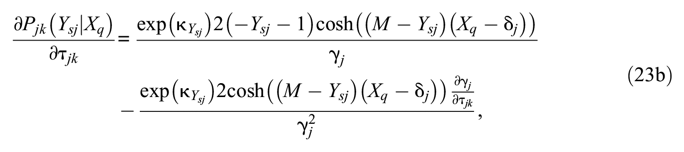
and


After the E-step, a maximization step (M-step) is performed: The likelihood equations (21 and 22) for each item are set to zero and solved for their roots (
Method
Simulation Study
The authors conducted a Monte Carlo simulation to examine parameter estimation requirements for the GHCM based on the MML-EM approach. Three factors were manipulated in a fully-crossed 5 × 2 × 2 experimental design: (a) sample size (50, 100, 200, 400, 800); (b) number of items (10, 20); (c) data type (dichotomous, four-option polytomous). Fifty replications were performed in each experimental condition.
Parameters for response data generation were selected based on previous studies with ideal point models (e.g., Carter & Zickar, 2011; Joo, Lee, & Stark, 2017; Koenig & Roberts, 2007; Roberts, Donoghue, & Laughlin, 2002; Roberts & Thompson, 2011). Location parameters (
EM Implementation
Initial values for the GHCM item parameters were chosen in accordance with previous ideal point model simulation studies (e.g., Andrich & Luo, 1993; de la Torre, Stark, & Chernyshenko, 2006; Roberts et al., 2000). Because the items in each measure were already sorted by their location parameters, and person parameters were sampled from a N(0,1) distribution, the initial location parameter for item 1 was set at −3 and successive items were assigned initial location values in increments of 6 / (J − 1), where J is total number of items in the measure. All initial threshold parameters were set at −1.
To perform the numerical integration in the E-step, 61 equally spaced quadrature points on the interval [−3, 3] were used. The likelihood of the response data was computed using the
Person Parameter Estimation
The expected a posteriori (EAP; Bock & Mislevy, 1982) method was chosen for estimating person parameters of the GHCM. In EAP, the person parameter estimates are obtained for each respondent by taking the mean of the posterior density of


where
Analysis
To assess the efficacy of GHCM parameter estimation, root mean square error (RMSE =
Results
Table 1 presents the overall parameter recovery statistics for the individual simulation conditions. For the four-option polytomous conditions, note that RMSE, BIAS, and SE of
GHCM Monte Carlo Study Results.
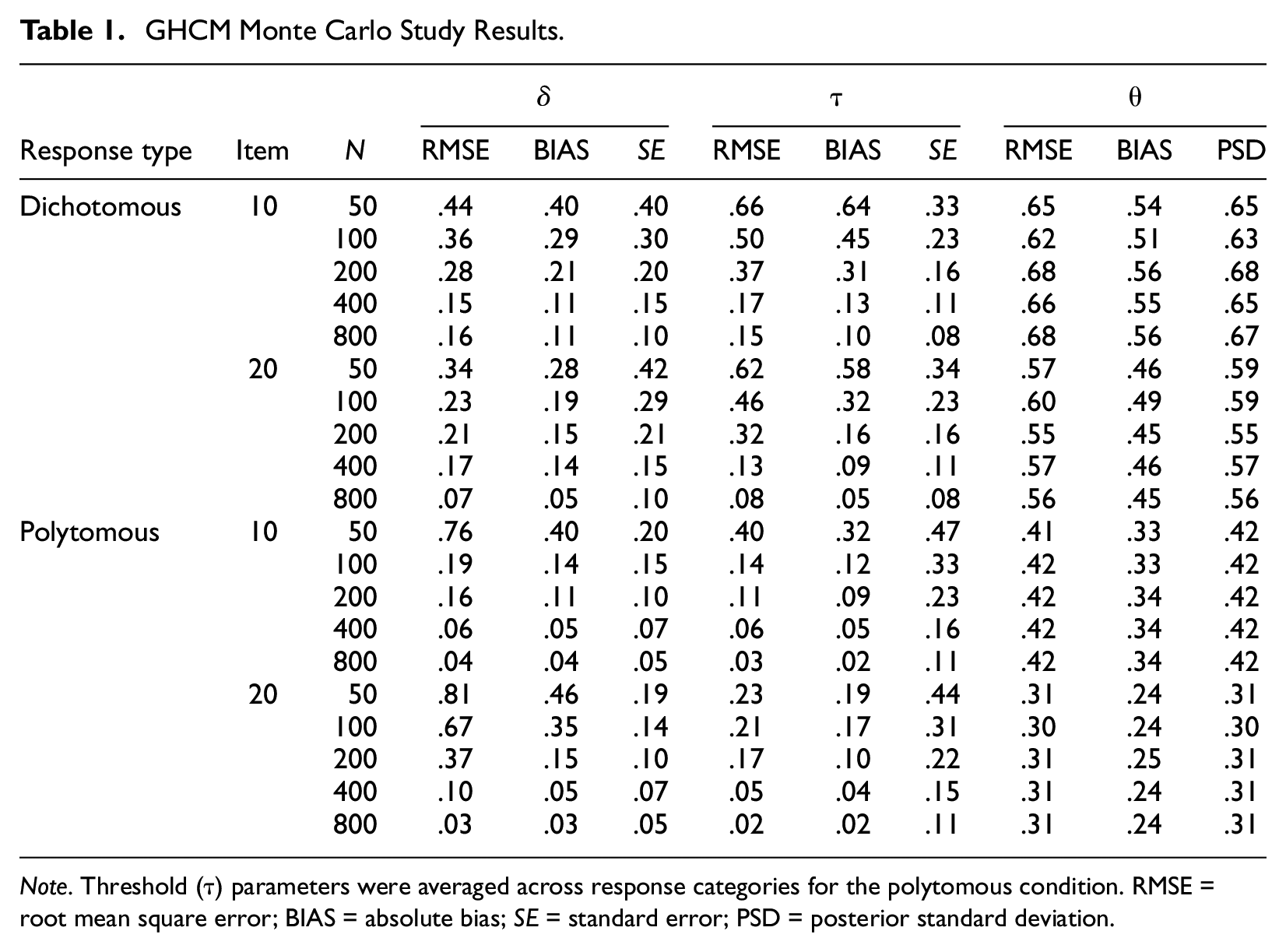
Note. Threshold (τ) parameters were averaged across response categories for the polytomous condition. RMSE = root mean square error; BIAS = absolute bias; SE = standard error; PSD = posterior standard deviation.
The detailed results in Table 1 show that the overall accuracy of GHCM item parameter estimates was a clear function of sample size. The magnitude of the three error measures (RMSE, BIAS, and SE) decreased as sample size increased, regardless of the item parameter in question. It is important to note that after the sample size reached 400, the increased precision afforded by larger samples began to wane. Note also that, with the sample size of 400, the parameter estimates of the GHCM were recovered well. For example, with 400 simulees, the marginal values of RMSE, BIAS, and SE across simulation conditions for
Overall item parameters were estimated better in polytomous conditions than in dichotomous conditions with equal sample size. For example, when the sample size was 400 and the number of items was 20, the BIAS of
In addition, person parameters were most accurately estimated with the 20-item polytomous data. As shown in Table 1, the accuracy of the person parameter estimates increased as the number of items increased, and better results were obtained with polytomous data than with dichotomous data. However, person parameter estimates were not influenced by sample size, which suggests robustness to item parameter estimation error as reported in previous research (e.g., Stark, Chernyshenko, & Guenole, 2011).
Real Data Example
To illustrate the application of the GHCM based on the MML-EM algorithm, the authors analyzed 493 responses to a four-option (0 = Strongly Disagree, 1 = Disagree, 2 = Agree, 3 = Strongly Agree), 20-item Orderliness scale (Chernyshenko, 2002). They expected that a sample size of 493 would be adequate for estimation based on the simulation findings. The initial location parameters were generated based on the item responses using the method described by Roberts and Laughlin (1996) and the initial threshold parameters were set at −1. For more information about the initial values for location parameters, readers may refer to the Appendix in Roberts and Laughlin (1996). The parameter estimates and their SEs for the complete set of items are presented in Table 2.
GHCM Item Parameters and Standard Errors for 20-Item Orderliness Scale.
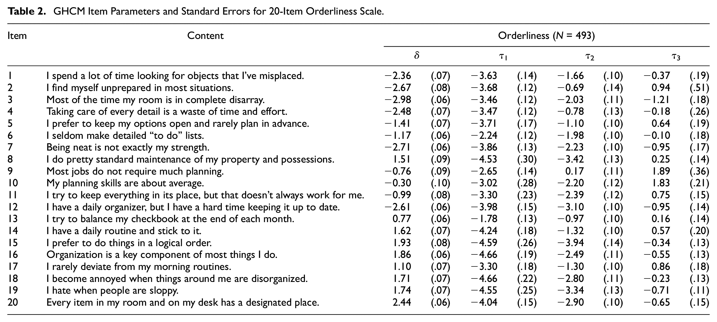
As shown in Table 2, the estimated values of
In addition, selected IRFs from this analysis are presented in Figure 3. In accordance with expectations, the IRFs for Items 9 and 13, which had moderate location parameters (–.76 and .77, respectively), exhibit marked folding (somewhat bell-shaped), whereas the IRFs for Items 4 and 18, which had more extreme location parameters (−2.48 and 1.71, respectively) exhibit only moderate folding at one end of the depicted trait range.

Selected IRFs from real data analysis using 20-item orderliness scale.
Discussion
This research was conducted to redirect attention toward a potentially useful ideal point model for noncognitive measurement in educational and organizational contexts. The authors developed an MML-EM algorithm for GHCM item parameter estimation and explored item properties and parameter recovery to address concerns raised in early ideal point personality research (Stark et al., 2000). They also presented example IRFs and IIFs to explore GHCM similarity to models that are more mathematically complex (e.g., GGUM; Roberts et al., 2000). Consistent with research on the GGUM (Roberts et al., 2002), they found that GHCM parameters were estimated better with polytomous data than with dichotomous data. However, improvements in item parameter estimation accuracy with samples larger than 400 were fairly small—a finding that should be encouraging to practitioners. In addition, their real data analysis showed that the estimation algorithm produced parameter estimates and SEs in accordance with their simulation findings, as well as with previous ideal point calibration studies using similar prior distributions (i.e., de la Torre et al., 2006).
Comparison With the GGUM
As noted in the introduction, the GHCM and GGUM have a number of features in common. As shown in Figures 1 and 2, the GHCM has IRFs and IIFs resembling the GGUM (Roberts et al., 2000). The IRFs of both models are bell-shaped and symmetric, and their IIFs are bimodal and symmetrical around |
To explore the similarity of the two models further, the authors examined the correspondence between GHCM and GGUM trait scores in their large sample (N = 800) conditions. They generated GGUM dichotomous and four-option polytomous response data using person parameters (thetas) sampled from a standard normal distribution and item parameters similar to those in previously published studies (e.g., Roberts et al., 2002). They fitted the GGUM and GHCM to those data and compared the resulting EAP theta estimates. Scatterplots showing the correspondence between the GGUM and GHCM theta estimates are presented in Figure 4. Across conditions, the correlations ranged from .76 to .96 and increased substantially as the number of items and categories increased, suggesting that the GHCM may be a viable alternative to the GGUM for measuring noncognitive constructs.

Correspondence between GHCM and GGUM person parameter (Theta) estimates.
For the model parameterization, however, there is a distinct difference between the GHCM and GGUM. Most notably, the GGUM includes a discrimination parameter along with location and threshold parameters, whereas the GHCM contains only location and threshold parameters. The GGUM is thus more flexible and can be seen as a more general model. In future research, it would be interesting to modify the GHCM by adding a discrimination parameter and compare model fit with the GGUM under various conditions.
Limitations and Future Research
Based on the findings of this study, the authors recommend that researchers use polytomous response formats and a calibration sample size of 400 when item parameter accuracy is a priority (e.g., in measurement equivalence studies). These recommendations are made while recognizing their study’s limitations. More specifically, this study and others have shown that ideal point model estimation is generally better with polytomous formats, but the authors only compared performance with two and four response options. Future research might consider expanding the number of options to five, six, or seven to cover the range of formats typically seen in applied research. Second, the authors used an MML-EM method to examine GHCM calibration requirements, but future studies may explore whether Markov chain Monte Carlo (MCMC; Patz & Junker, 1999) methods, which do not require first- and second-order partial derivatives, are more effective with samples of 400 and smaller. Alternatively, the marginal maximum a posteriori (MMAP) method can be developed for the GHCM, given that MMAP strategy for the GGUM reduces tradeoffs that are often observed between location and threshold parameters (Roberts & Thompson, 2011). Third, because this study presented GHCM IIFs, it may be useful to examine the GHCM as a basis for computerized adaptive testing (CAT).
In summary, the authors hope that this study serves as a catalyst for future ideal point modeling and application research. They encourage practitioners to explore the GHCM as an alternative to other ideal point models for ordered categorical responses and perhaps develop generalizations to address faking and other types of aberrant responding associated with noncognitive measurement.
Supplemental Material
APM-17-03-060.R3_Online_Supplemental_Material_(1) – Supplemental material for Item Parameter Estimation With the General Hyperbolic Cosine Ideal Point IRT Model
Supplemental material, APM-17-03-060.R3_Online_Supplemental_Material_(1) for Item Parameter Estimation With the General Hyperbolic Cosine Ideal Point IRT Model by Seang-Hwane Joo, Seokjoon Chun, Stephen Stark, and Olexander S. Chernyshenko in Applied Psychological Measurement
Footnotes
Authors’ Note
The current affiliation for the Author ‘Olexander S. Chernyshenko’ is ‘University of Western Australia, Australia’.
Declaration of Conflicting Interests
The author(s) declared no potential conflicts of interest with respect to the research, authorship, and/or publication of this article.
Funding
The author(s) received no financial support for the research, authorship, and/or publication of this article.
Supplemental Material
Supplemental material is available for this article online.
References
Supplementary Material
Please find the following supplemental material available below.
For Open Access articles published under a Creative Commons License, all supplemental material carries the same license as the article it is associated with.
For non-Open Access articles published, all supplemental material carries a non-exclusive license, and permission requests for re-use of supplemental material or any part of supplemental material shall be sent directly to the copyright owner as specified in the copyright notice associated with the article.
