A Law of Comparative Preference: Distinctions Between Models of Personal Preference and Impersonal Judgment in Pair Comparison Designs

Abstract

The pair comparison design for distinguishing between stimuli located on the same natural or hypothesized linear continuum is used both when the response is a personal preference and when it is an impersonal judgment. Appropriate models which complement the different responses have been proposed. However, the models most appropriate for impersonal judgments have also been described as modeling choice, which may imply personal preference. This leads to potential confusion in interpretation of scale estimates of the stimuli, in particular whether they reflect a substantive order on the variable or reflect a characteristic of the sample which is different from the substantive order on the variable. Using Thurstone’s concept of a discriminal response when a person engages with each stimulus, this article explains the overlapping and distinctive relationships between models for pair comparison designs when used for preference and judgment. In doing so, it exploits the properties of the relatively new hyperbolic cosine model which is not only appropriate for modeling personal preferences but has an explicit mathematical relationship with models for impersonal judgments. The hyperbolic cosine model is shown to be a special case of a more general form, referred to in parallel with Thurstone’s Law of Comparative Judgment, as a specific law of comparative preference. Analyses of two real data sets illustrate the differences between the models most appropriate for personal preferences and impersonal judgments in a pair comparison design.

Keywords

Law of Comparative Judgment pair comparisons preference and choice unfolding single-peaked response function

Introduction

The pair comparison (PC) design has a long history originating from psychophysics where the psychological sensations of stimuli were related to their known physical magnitudes (Bock & Jones, 1968). In the 1920s, Thurstone (1927a, 1927b) formalized the response model for PC designs when the stimuli had no physical counterpart, generally performances or attitude statements that expressed different degrees of attitude. Thurstone called this formalization the Law of Comparative Judgment (LCJ) with slightly different cases, successively specializing from the most general form the attribution of errors. The principles relevant for this article hold for all cases of the LCJ, but because the mathematical features of Case V permit it to be used efficiently in relating models in this article, all references are to this case. The LCJ(V) implies that error variances of responses of persons to items are homogeneous among persons and items, which is formalized later in the article and is the most common form applied.

Three features are central to the LCJ(V): First, the stimuli are located on a latent continuum with different magnitudes. Second, when a person engages with each stimulus there is a sensation called a discriminal process which gives rise to a discriminal response. The selection then depends on the relative magnitude of the discriminal responses to the two stimuli. Third, the judgment is independent of any personal preference for any stimulus and is therefore an impersonal judgment. The features are elaborated in the section “Thurstone’s Monotonic Latent Discriminal Response Process and the LCJ.”

Based on a different rationale from Thurstone’s, Bradley and Terry (1952) and Luce (1959) proposed a probabilistic logistic model for the PC design, known as the Bradley–Terry–Luce Model (BTLM), rather than the cumulative normal used by Thurstone. However, Andrich (1978) showed that with minor modifications of the assumptions regarding the discriminal response and the numerical specification, the model was equivalent to the LCJ(V). Therefore as a further simplification for this article, all relevant interpretations of the BTLM for this article will be understood to apply to the LCJ(V), and in turn to the general LCJ. The BTLM is also made explicit in the section “Thurstone’s Monotonic Latent Discriminal Response Process and the LCJ.”

Because the BTLM is equivalent to the LCJ(V), it has been used to model (impersonal) comparative judgments, and because Luce (1959) called it a choice model, it has been used to model (personal) comparative preferences. In addition, Bock and Jones (1968) treated the concepts of judgment and choice as equivalent. However, Coombs (1964) argued that because of individual differences common in many cases when making a choice between stimuli, the BTLM was unrealistic in many situations. Thus, different terminology regarding preference and judgment has resulted in different models being applied to the same PC design and the same model being applied to different PC designs.

To make the difference between an impersonal judgment and personal preference concrete, consider the stimuli to be cups of coffee identical in all respects except for fine gradations of the amount of sugar in them. Two different instructions can be given for making comparative selections.

Instruction I: Select the cup in each pair which has more sugar. This selection is to be independent of each person’s preference, and therefore is an impersonal, comparative judgment.

Instruction II: Select the cup in each pair that you prefer. This selection is intended to be dependent on each person’s preference, and therefore is a personal, comparative preference.

The terms preference and choice which imply interpersonal differences seem to be used interchangeably. However, because choice is associated with the BTLM, the rest of this article uses preference. In addition, when a comparison is not specifically a personal preference or an impersonal judgment, the neutral term select is used.

The purpose of this article is to clarify the distinction between a comparative process which is an impersonal judgment and one which is a personal preference, and to relate the appropriate model and interpretation to the appropriate instruction to the respondents in the PC design. It is emphasized that the purpose is not to merely describe the differences but to explain them. The explanation is based on explicating and using, as a basis, Thurstone’s concept of a discriminal process and response. In explaining the relationships between the models, the article uses the properties of the relatively new hyperbolic cosine model (HCM). The HCM is appropriate for modeling personal preferences in a PC design, and has an explicit mathematical relationship with the BTLM. The article is not concerned with methods of estimation and the like which are well described in the literature, nor with a review of the vast literature on PC designs and models for them. Instead, it focuses on first principles in clarifying two distinct sets of instructions (preference, judgment) in the PC design and two fundamental models (LCJ(V)/BTLM, HCM) that are most appropriate for each, and the relationship between them. To consolidate the different interpretations of the models, two sets of real data are analyzed by both models.

The rest of the article is structured as follows: Section “Thurstone’s Monotonic Latent Discriminal Response Process and the LCJ” provides the rationale for Thurstone’s LCJ and his specific Case V which is relevant for impersonal judgments and which leads to the equivalent BTLM; section “The Bradley–Terry–Luce Rationales for the Same Model as the Logistic LCJ(V)” provides Bradley and Terry’s, and Luce’s, rationales for the BTLM; section “A Single-Peaked Discriminal Response” describes the HCM for personal preference; section “Examples” provides two examples of analyses of data using both the HCM and the BTLM; and section “Summary and a General LCP” is a summary, and proposes that in parallel to Thurstone’s LCJ, the HCM can be characterized as a special case of The Law of Comparative Preference (LCP).

Thurstone’s Monotonic Latent Discriminal Response Process and the LCJ

Thurstone postulated that when a person (called a subject) engaged with stimuli,

. . . each stimulus gives rise to a momentary subjective value . . . When two stimuli are compared by the subject, the stimulus whose momentary value is greater is the one which seems larger to the subject. (Bock & Jones, 1968, p. 3)

The momentary subjective value is Thurstone’s discriminal process which gives a momentary discriminal response. Thurstone (1927a) implied a personal characteristic in the discriminal response:

If you look at two handwriting specimens in a mood slightly more generous and tolerant than ordinarily, you may perceive a degree of excellence in specimen A a little higher than its mean excellence. But at the same moment specimen B is judged a little higher than its average or mean excellence for the same reason. (p. 268)

Clearly, Thurstone indicated a personal characteristic (generosity) in the discriminal responses. However, the consequence of the same generosity in comparing two pieces of handwriting indicates that Thurstone assumed the comparison to be a judgment of the quality of handwriting, not a reflection of the person’s generosity for any kind of handwriting. In addition to achievement items, Thurstone (1928) applied the LCJ to scale items that measured attitude. Andrich (1978) formalized the above assumption and showed that, in comparison, the person parameter characterizing generosity was eliminated. An alternative approach to this elimination is briefly reviewed below.

First, Andrich showed that on replacing the cumulative normal with the virtually equivalent logistic, the discriminal response in the LCJ(V) was equivalent to the formulation:

P_{ni 1} = \Pr {X_{ni} = 1; β_{n}, δ_{i}} = \frac{\exp (δ_{i} - β_{n})}{[1 + \exp (δ_{i} - β_{n})]},

where $X_{ni}$ is a random variable that can take on values $x = 0, 1$ for a negative and a positive discriminal response, respectively; $β_{n}$ is the characteristic of person $n$ when engaging with stimulus $i$ of intensity $δ_{i}$ ; and that $P_{ni 0} = 1 - P_{ni 1}$ . For convenience, and to ensure that the more intense the stimulus and the more sensitive the person, the higher probability of a positive response, $β_{n}$ is termed person $n$ ’s insensitivity in Equation 1, which increases to the right in Figure 1.

Figure 1.

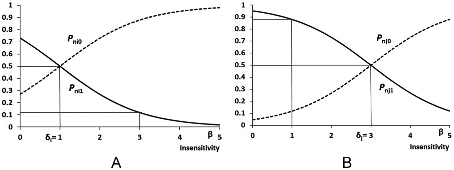
The probability of positive and negative discriminal responses to stimuli i (Panel A) and j (Panel B) from the logistic form of the LCJ(V).

Here, the implications of Equation 1 for the PC Design I are shown above. Suppose again that the comparisons are made with cups of coffee with varying amounts of sugar. In the discriminal response for each cup, the greater the amount of sugar and the more sensitive the person, the greater the probability of detection. Figure 1 shows the probability $P_{ni 1}$ of detecting sugar according to Equation 1 for cups with $δ_{i} = 1.00, δ_{j} = 3.00$ units of sugar as a function of $β$ . The probability $P_{ni 0}$ of not detecting sugar is also shown. For example, if $β_{n} = 1$ on the same scale as sugar, the probability of detecting $δ_{i} = 1.00$ is exactly $P_{ni 1} = . 5$ while the probability of detecting $δ_{j} = 3.00$ is greater, $P_{nj 1} = . 881$ . Corresponding probabilities follow if $β_{n} = 3$ .

The probability curves in Figure 1 are monotonic, and the response process is said to be cumulative. If $β$ represents proficiency and $δ_{i}$ the difficulty of item $i$ in assessing this proficiency, then Equation 1 is a well-known dichotomous Rasch (1960) model with the relationship between $β_{n}$ and $δ_{i}$ opposite to that in Equation 1 of the Rasch model. The difference $β_{n} - δ_{i}$ then implies that the greater the proficiency $β_{n}$ relative to difficulty $δ_{i}$ , the greater the probability of a positive (correct) response.

In comparing stimuli $i$ and $j$ , the discriminal response space is composed of subspaces ${(0, 0)}$ (detecting neither), ${(1, 1)}$ (detecting both), and ${(1, 0), (0, 1)}$ (detecting one and not the other). Judging that one stimulus has more of the property than the other implies the subspace ${(1, 0), (0, 1)}$ . For example, the probability of detecting sugar in $i$ but not in $j$ is given by

\Pr {(1, 0) | {(1, 0), (0, 1)}} = \frac{P_{ni 1} P_{nj 0}}{(P_{ni 1} P_{nj 0} + P_{ni 0} P_{nj 1})} .

Conditioning on the subspace ${(1, 0), (0, 1)}$ is not to be taken literally—for example, a person may detect sugar in both cups, but in selecting one, it is as if the person detected sugar in one and not the other. Let $P_{nij}$ be the probability that person $n$ selects $i$ over $j$ . Then, inserting $P_{ni 1}, P_{ni 0}, P_{nj 1}, P_{nj 0}$ from Equation 1 into Equation 2 and simplifying gives

P_{nij} = \frac{\exp (δ_{i} - δ_{j})}{[1 + \exp (δ_{i} - δ_{j})]} .

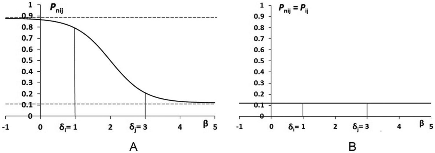
Equation 3 does not include $β_{n}$ , showing that the probability of the comparative judgment is only a function of the stimuli. Therefore, the authors may omit the person subscript $n$ and write $P_{nij} = P_{ij}$ . Figure 2, Panel B, shows the probability of selecting $δ_{i} = 1$ over $δ_{j} = 3$ . Clearly, independent of $β_{n}$ , this probability is a straight line. In anticipation of relating this probability to that of a comparative preference based on an analogous derivation, Panel A of Figure 2 shows the probability of selecting $δ_{i} = 1$ ahead of $δ_{j} = 3$ as a function of $β_{n}$ according to the HCM.

Figure 2.

Probability of selecting $i$ over $j$ as a function of the person parameter $β$ in the HCM (Panel A) and the BTLM (Panel B).

In the context in which psychological values of statements used to assess attitudes toward a range of topics (e.g., capital punishment) were estimated, Thurstone (1928) emphasized,

If a scale is to be regarded as valid, the scale values of the statements should not be affected by the opinions of the people who help to construct it . . . the scaling method must stand such a test before it can be accepted as being more than a description of the people who construct the scale. (p. 547)

Thus, in the scale construction stage, when relative locations of statements are estimated on a continuum, personal opinions are not expected to have a role. However, if they did in this stage, then the scale values would reflect the sample of persons making the comparisons. This reference to descriptions of samples leads to the Bradley–Terry and Luce formulation.

The Bradley–Terry–Luce Rationales for the Same Model as the Logistic LCJ(V)

In Bradley and Terry (1952) and Bradley (1976), the probability $P_{ij}$ that stimulus $i$ is selected over $j$ is defined by Equation 4:

P_{ij} = \frac{π_{i}}{(π_{i} + π_{j})},

where $π_{i}, π_{j}$ were termed treatment parameters of $i$ and $j$ : The denominator $π_{i} + π_{j}$ ensures that $P_{ij} + P_{ji} = 1$ . Notice that immediately, rather than by elimination as in the Thurstone formulation (Andrich, 1978), there is no person parameter in Equation 4. Bradley (1976) explained that $π_{i}, π_{j}$ were invariant with respect to different persons.

Independently, Luce (1959) developed the same model for the PC design and referred to it as an axiom of choice. This axiom specifies that in the choice of stimulus $i$ from a set of multiple stimuli, $j = 1, 2, \dots, J$ , the ratio $π_{i} / π_{j}$ remains invariant in comparisons with other stimuli in the set.

Let $π_{i} = \exp (δ_{i}), π_{j} = \exp (δ_{j})$ . Then on simplification, Equation 4 becomes

P_{ij} = \frac{\exp (δ_{i} - δ_{j})}{[1 + \exp (δ_{i} - δ_{j})]},

which is identical to Equation 3, the logistic form of the LCJ(V), and is the BTLM.

The absence of a person parameter in Equation 5 is legitimate only for impersonal judgments, in which case the estimates for the stimuli reflect their intrinsic relative values on the continuum. However, when applied to personal preferences the person parameter is intrinsic to the responses and cannot be eliminated from the responses. Then, the estimates of $δ_{i}, δ_{j}$ in the BTLM reflect the choice disposition of the sample. The way personal preferences analyzed with the BTLM play out is shown with the examples in the article.

A Single-Peaked Discriminal Response

As indicated above, Coombs (1964) considered that the BTLM is unrealistic in situations of individual preference and choice. Coombs’s alternative response processes were deterministic. In this study, the authors proceed immediately with a probabilistic formulation for a comparative preference. They begin again with a discriminal response when a person engages with each stimulus but one in which the response function is single peaked rather than monotonic. Such a function reflects a preference and is said to be unfolding rather than cumulative, a term illustrated later in the article. For example, in the case of amounts of sugar in cups of coffee, the person will reject those that have too much and too little for the person’s liking. In this formulation, each person is hypothesized to like an ideal amount of sugar, formalized as an ideal point. Then, if a person’s ideal point is three units of sugar, a cup with this many units has the highest probability of receiving a positive response, and those with more and less sugar than the ideal point have a lower probability. This principle is reflected in the single-peaked response functions shown in Figure 3, which contrasts with the monotonic functions shown in Figure 1. Figure 3 also shows the complementary probabilities of a negative response. The contrast between the discriminal responses in Figures 1 and 3 is the basis of the difference between judgment and preference models in PC designs.

Figure 3.

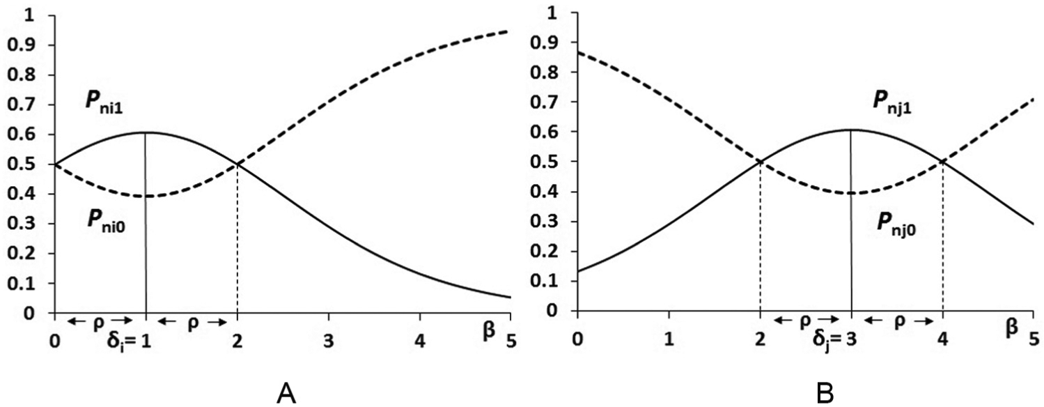
The probability of positive and negative discriminal responses to stimuli i (Panel A) and j (Panel B) from the HCM.

The specific form of the single-peaked response functions in Figure 3 is given as (Andrich, 1995)

P_{ni 1} = \Pr {X_{ni} = 1; β_{n}, δ_{i}, ρ_{i}} = \frac{\cosh (ρ_{i})}{[\cosh (ρ_{i}) + \cosh (β_{n} - δ_{i})]},

where $X_{ni}$ is a random variable taking on values $x = 0, 1$ for a negative and a positive response, respectively, $β_{n}$ is the ideal point for person $n$ when engaging with stimulus $i$ of intensity $δ_{i}$ , $ρ_{i}$ is the latitude of acceptance of the stimulus and is the point of intersection of the probabilities of a positive and a negative response, and $\cosh (x)$ is the hyperbolic cosine function $\cosh (x) = (\exp (- x) + \exp (x)) / 2$ . The model, termed the hyperbolic cosine, was derived from Andrich and Luo (1993) and applied to real data. That derivation will not be repeated here where the focus is on models for data generated from PC designs. The model was further developed by Luo (1998, 2001) and is summarized by Andrich (2016b).

In parallel to the construction of the BTLM based on a monotonic function for the discriminal response in the section “Thurstone’s Monotonic Latent Discriminal Response Process and the LCJ,” consider a construction of a comparative preference based on the single-peaked discriminal response of Equation 6. The derivation follows the pattern of the monotonic discriminal responses with the responses now being acceptable and unacceptable rather than detecting or not detecting. Thus, in selecting one of two cups of coffee, the discrete discriminal response subspaces are ${(0, 0)}$ (both unacceptable), ${(1, 1)}$ (both acceptable), and ${(1, 0), (0, 1)}$ (one acceptable and one not). Selecting one implies the conditional subspace ${(1, 0), (0, 1)}$ . For example, the probability of preferring $i$ to $j$ is again given by

\Pr {(1, 0) | {(1, 0), (0, 1)}} = \frac{P_{ni 1} P_{nj 0}}{(P_{ni 1} P_{nj 0} + P_{ni 0} P_{nj 1})} .

The conditioning on the subspace ${(1, 0), (0, 1)}$ is also again not to be taken literally—for example, a person may find both cups more or less acceptable, but in selecting one, it is as if the person found that one acceptable and not the other. Let $P_{nij}$ be the probability that person $n$ selects $i$ ahead of $j$ . Then, inserting $P_{ni 1}, P_{ni 0}, P_{nj 1}, P_{nj 0}$ from Equation 6 into Equation 2, and assuming that latitudes of acceptances are equal, $ρ_{i} = ρ_{j}$ , it is simplified as follows (Andrich, 1995):

P_{nij} = \Pr {(1, 0) | {(1, 0), (0, 1)}} = \frac{\cosh (β_{n} - δ_{j})}{[\cosh (β_{n} - δ_{i}) + \cosh (β_{n} - δ_{j})]} .

Unlike Equation 3 of the logistic form of the LCJ(V) and the BTLM, Equation 8 retains the person parameter $β_{n}$ . Accordingly, it is a model for personal preference. The probability of Equation 8 for two fixed values of $δ_{i}, δ_{j}$ as a function of the ideal point $β$ is shown in Figure 2, Panel A. Specifically, the greater person n’s ideal point $β_{n}$ , the more likely the stimulus closer to the ideal point will be selected. Its contrast with the BTLM of Equation 3 in Figure 2 Panel B is clear.

Andrich (1995) gave some properties of the HCM as well as methods of estimating the parameters. One boundary condition is that if $δ_{i} = δ_{j}$ and if the ideal point $β_{n} = (δ_{i} + δ_{j}) / 2,$ then $P_{nij} = P_{nji} = 0.5$ . These probabilities are consistent with intuition. Second, and particularly relevant for this article, is that as the person’s ideal point becomes very large in magnitude relative to the locations of the two stimuli, the probability of selecting one over the other reaches an asymptote which is a function only of the difference between the two stimuli. Specifically,

\underset{lim β \to \infty}{P_{nij}} = \frac{\exp (δ_{i} - δ_{j})}{[1 + \exp (δ_{i} - δ_{j})]} .

Equation 9 is identical to the BTLM of Equations 4 and 5. Thus, the HCM has a limiting case, when a person’s ideal point is extreme, in which only the locations of the stimuli play a role and the model is the BTLM. This limiting probability is shown by the asymptote in Panel A of Figure 2.

To consolidate the contrast between the HCM and the BTLM, analyses of two examples of pairwise preference type data in which the discriminal response is single peaked with both the HCM and the BTLM are reported. The estimation method for the HCM uses joint maximum likelihood, and requires iterations on the person and the item parameters successively. The method is described in detail by Andrich (1995). The software used was RUMMFOLDpp (Andrich & Luo, 1997).

Examples

This section provides two examples in which the HCM is the correct model of analysis but which can be analyzed using the BTLM. The data for both examples came from the same sample. This sample consists of 187 students, 67 predominantly third-year primary teacher education students (56 females and 11 males), 68 predominantly second-year psychology students (43 females and 25 males) at Murdoch University in Australia, and 52 predominantly second-year commerce students (24 females and 28 males) from the University of Western Australia.

Example 1: Stimuli With Known Values on a Continuum

In Example 1, the students were asked to indicate which of each pair of salaries from the set Aus$25,000, Aus$30,000, Aus$35,000, Aus$40,000, and Aus$45,000 they were most likely to earn in their first year of employment. In these comparisons, students are not literally selecting their preferred salaries. Clearly, it can be assumed that they would prefer to have a higher salary. There are two reasons for using the example in this article. First, the discriminal response is single peaked—that is, on engaging with a particular salary, the latent response is to accept the salary most likely and reject salaries that are greater or smaller than this salary. Second, the salaries have independent values on a unidimensional continuum, more or less as in psychophysical examples, and estimated psychological values can be compared with these values.

Table 1 shows the scale values estimated from both the HCM and the BTLM together with the frequency with which each salary was selected when summed over all comparisons, and the χ² test of fit statistics which compare the observed with the expected frequency under the model. Figure 4 shows plots of the scale estimates of the HCM and the BTLM against the known salaries. For purposes of visual inspection, a linear regression line is shown for the former and a quadratic regression curve for the latter.

Table 1.

Psychological Scale Values of Salaries From the HCM and the BTLM.

Salary	Aus$25,000	Aus$30,000	Aus$35,000	Aus$40,000	Aus$45,000
HCM	−6.804	−3.998	0.338	3.669	6.795
BTLM	−0.030	0.657	0.697	−0.197	−1.123
Selections	356	496	504	322	150
HCM	$χ^{2} = 2.370, 6 df, p = . 833$		BTLM	$χ^{2} = . 250, 6 df, p = . 999$

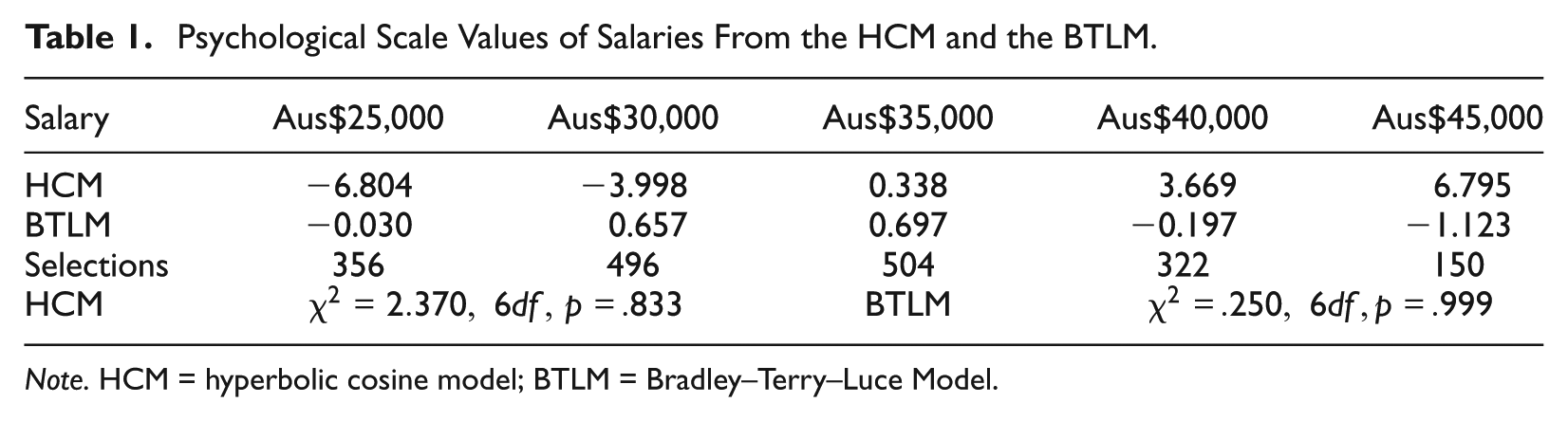
Note. HCM = hyperbolic cosine model; BTLM = Bradley–Terry–Luce Model.

Figure 4.

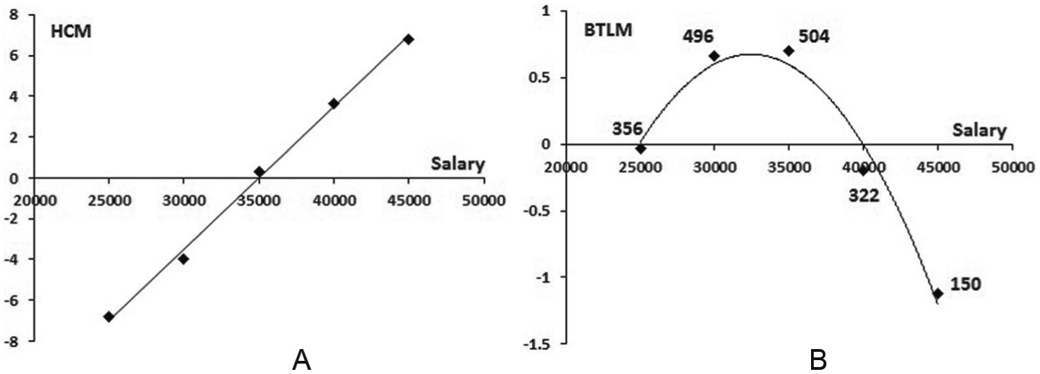
Scale values from the HCM (Panel A) and the BTLM (Panel B) against known salaries with the number of selections of each salary shown in Panel B.

First, it is evident that the fit is excellent with both models. Second, the HCM scale values are in the same order as the salaries, and the relative distances are equivalent. Thus, there is no evidence of a systematic shrinking or stretching of the scale. On the contrary, the BTLM scale values have a curvilinear relationship with salaries. It is evident from Table 1 that the salary of Aus$35,000 was the one selected most frequently (504 times), closely followed by Aus$30,000 (496 times). The scale values of the BTLM follow the frequency of selection virtually, perfectly, linearly with a correlation of 1.000. It is clear from this example that the BTLM scales the salaries in the order of the frequency of their selection and not in the order of their known values on a continuum.

Two further points of contrast arise between the BTLM and HCM. First, the scale values from the BTLM are referenced to a population, and indicate the degree to which each salary is selected and does not recover any a priori order as does the HCM. Second, the curvilinear shape of the scale values from the BTLM relative to the known salaries shows that they have been folded around the most frequent selection, that is, the sample’s not a person’s ideal point, thus losing the a priori order of the salaries. This is the rationale that led Coombs (1964) to question the appropriateness of the BTLM for preference data and led to his techniques of unfolding the scale values at the personal level. In contrast to the BTLM which reflects the folding at the sample level, the HCM immediately unfolds the responses at each person’s ideal point.

Example 2: Stimuli With Unknown Values but With an Order on a Continuum

In the second example, the students were asked to select in a PC design which of the following five grades they were most likely to achieve in the subject they were studying in the class in which they were participating at the time: High Distinction, Distinction, Credit (pass), Pass (regular), or Conceded (pass). These grades were assigned to students at the time of the data collection and are typical in Australian universities. Students were not asked to indicate the grade they literally preferred. However, the discriminal response is single peaked—if a student thought he or she would receive a particular nonextreme grade, that grade would have the highest probability of a positive response with grades either higher or lower having a lower probability.

Although they have no known specific a priori values, there is an a priori order to the grades from Conceded to High Distinction (High D). Table 2 shows the scale values estimated from both the HCM and the BTLM together with the frequency with which each salary was selected when summed over all comparisons and a χ² test of fit. Figure 5 shows the plot of the HCM values against hypothesized equal distances between the grades (Panel A) and the plot of the BTLM grades against the HCM grades (Panel B). For ease of visual inspection only, the latter has a quadratic graph interpolated.

Table 2.

Estimated Scale Values for Grades From the HCM and the BTLM.

Grade	Conceded	Pass	Credit	Distinction	High D
HCM	−9.313	−5.050	−1.963	6.314	10.020
BTLM	−1.494	0.108	1.085	0.785	−0.507
Selections	111	381	558	509	268
HCM	$χ^{2} = 2.805, 6 df, p = . 834$		BTLM	$χ^{2} = 0.600, 6 df, p = . 996$

Note. HCM = hyperbolic cosine model; BTLM = Bradley–Terry–Luce Model.

Figure 5.

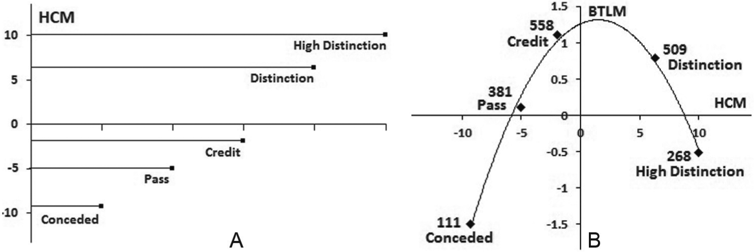
Scale values from the HCM (Panel A) between grades and the BTLM (Panel B) against the HCM values for the grades with the number of selections of each grade shown in Panel B.

The test of fit is again excellent with both models. The estimated values from the HCM, which are in the a priori order, show relevant interpretations. Although distances, visualized on the vertical axis, are somewhat similar between successive grades, the distance between Credit and Distinction is substantially greater. That students perceive this as the greatest distance between successive grades is entirely plausible.

To relate the values from the BTLM (which are not in the a priori order) to those from the HCM (which are in the a priori order), Figure 5 also shows the BTLM values plotted against the HCM values. As with Example 1, the BTLM values show a single-peaked relationship with grades in their a priori order and psychological values from the HCM.

The single-peaked relationship between the BTLM and the HCM values shows the folding of the former around the sample’s most frequently selected grade, that of Credit. Then relative to this value, estimates of other values fold by having lower scale values on either side of Credit. In the HCM, the scale values are immediately unfolded by accounting for individual differences.

This example consolidates evidence from Example 1 with salaries that the scale values from the BTLM do not recover the a priori order of stimuli when the response process is that of Design II in which the instruction is to select the stimulus based on a person’s preference and the discriminal response is single peaked. Instead, the BTLM analysis of such data gives scale values that reflect the relative frequency of selection of each stimulus, and in taking no account of individual differences the scale values explicitly characterize the sample.

Figure 6 shows the plot of the frequency of selection of each stimulus and the scale value from the BTLM for Examples 1 (Panel A) and 2 (Panel B). It shows that the relationship with the frequency is virtually linear.

Figure 6.

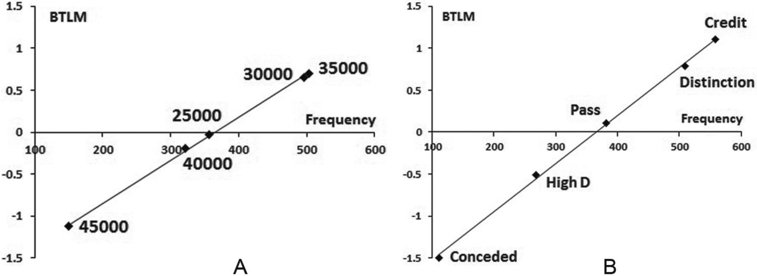
Scale values from the BTLM plotted against the frequency of selection of each stimulus for Example 1 (Panel A) and Example 2 (Panel B).

Finally from the results, Figure 7 shows the students’ ideal point estimates from the HCM for both examples and confirms substantial individual differences. These differences are accounted for, and can be estimated, by the HCM analysis, while they are irrelevant to the BTLM analysis.

Figure 7.

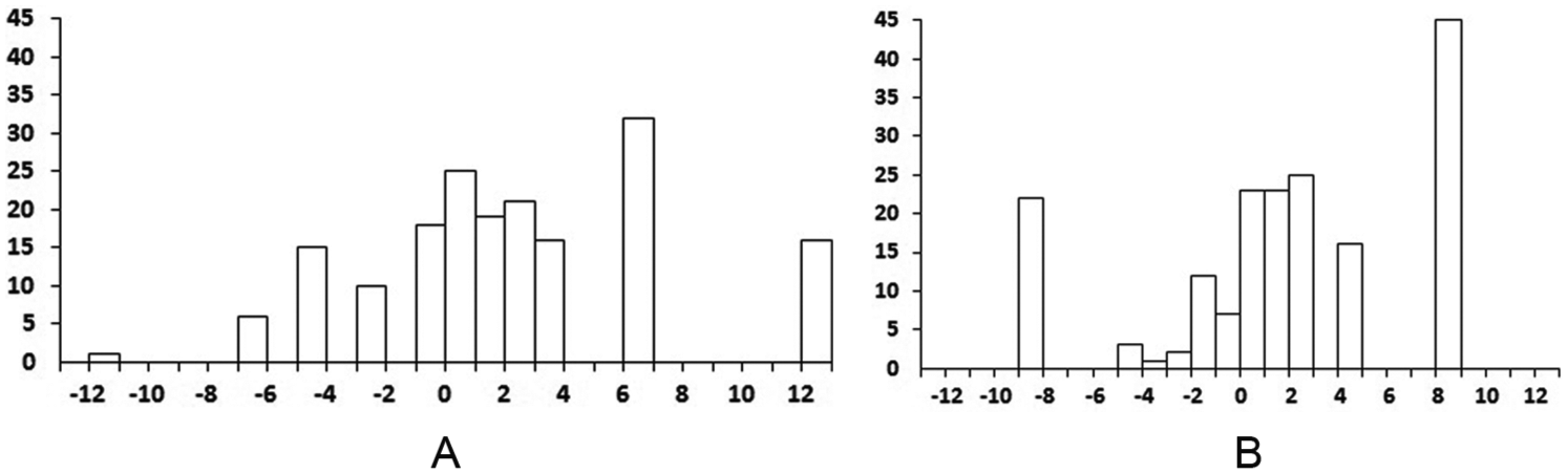
Distribution of persons from the HCM: Grades (Panel A); salaries (Panel B).

The classical test theory concept of reliability can be applied to the estimates from the HCM (Andrich, 2016a; Green, Bock, Humphreys, Linn, & Reckase, 1984). The concept is the ratio, $r_{β β}$ , of the estimated true variance, ${\hat{σ}}_{β}^{2}$ , of the sample divided by the total variance, the sum of the estimated true and error variance, ${\hat{σ}}_{β}^{2} + {\hat{σ}}_{e}^{2}$ . This is given by

r_{β β} = \frac{{\hat{σ}}_{β}^{2}}{{\hat{σ}}_{β}^{2} + {\hat{σ}}_{e}^{2}} = \frac{{\hat{σ}}_{\hat{β}}^{2} - {\hat{σ}}_{\hat{e}}^{2}}{σ_{\hat{β}}^{2}},

where ${\hat{σ}}_{\hat{β}}^{2}$ is the estimated variance of the estimated locations of the persons and ${\hat{σ}}_{\hat{e}}^{2}$ is the average, squared, standard error of measurement estimate for each person, where both ${\hat{σ}}_{\hat{β}}^{2}$ and ${\hat{σ}}_{\hat{e}}^{2}$ are available from any joint maximum-likelihood analysis. It is evident from Figure 7 that there are extreme cases at both ends of the continuum for both the salaries and the grades examples. Even though they have a finite estimate, these cases are essentially off the scale having a pattern that is extreme in its choices. As expected, these estimates have extremely large standard errors. If these extremes are eliminated because they do not reflect how reliably person locations are separated for the nonextreme cases, then the reliability indices according to Equation 10 are .808 and .761 for salaries and grades, respectively.

Summary and a General LCP

The theoretical analysis of Designs I and II above and the relevant models shows the following. First, if the instruction is to compare the stimuli and to select the one judged to have more of a relevant property as in Design I, then the discriminal response is monotonic as a function of the person–stimulus difference. Then, the psychological scale values can be related to an a priori order on a continuum, and the relevant model is the BTLM (effectively the LCJ(V) which is a special case of the general LCJ). In such an analysis, there is no information about individual differences in generosity or harshness. Second, if the instruction is to compare the stimuli and to select the one preferred with respect to a relevant property as in Design II, then the discriminal response is single peaked as a function of the person–stimulus difference. Then, the psychological scale values can be related to an a priori order on a linear continuum with the ideal points estimated, and the relevant model of analysis is the HCM.

Therefore, in constructing a PC design and deciding which model is the most relevant, the key is deciding the form of the discriminal response when a person engages with a stimulus—is it monotonic or is it single peaked?

It is relevant to note that to measure attitudes, Thurstone employed both concepts. He used the LCJ to first scale the locations of statements. Then to measure attitudes, he implied a single-peaked response process by taking the mean of the statement locations that a person agreed to. In an HCM analysis, the scale values of the items and the attitudes of the persons are obtained simultaneously. Accordingly, in parallel with the formulation of the LCJ, it was suggested that the HCM can claim to be a special case of a LCP. It is a special case of the general model:

P_{nij} = \frac{ψ (β_{n} - δ_{j})}{[ψ (β_{n} - δ_{i}) + ψ (β_{n} - δ_{j})]},

where $ψ (a)$ , termed the operational function, is a single-peaked response function (Luo, 1998). The function $ψ (a)$ specifically reflects a single-peaked discriminal response, in contrast to the monotonic latent discriminal response which leads to the BTLM and the LCJ(V). Another special case of the LCP (Luo, 1998) is based on the square logistic and takes the form

P_{nij} = \frac{\exp {(β_{n} - δ_{j})}^{2}}{[\exp {(β_{n} - δ_{i})}^{2} + \exp {(β_{n} - δ_{j})}^{2}]} .

Equation 11 is a general form into which all known models for pairwise preferences which take personal differences into account can be cast (Luo, 1998).

Footnotes

Declaration of Conflicting Interests

The author(s) declared no potential conflicts of interest with respect to the research, authorship, and/or publication of this article.

Funding

The author(s) disclosed receipt of the following financial support for the research, authorship, and/or publication of this article: The research for this article was supported in part by grants from the Australian Research Council and by Pearson.

References

Andrich

(1978). Relationships between the Thurstone and Rasch approaches to item scaling. Applied Psychological Measurement, 2, 449-460.

Andrich

(1995). Hyperbolic cosine latent trait models for unfolding direct-responses and pairwise preferences. Applied Psychological Measurement, 19, 269-290.

Andrich

(2016a). Accounting for local dependence with the Rasch model: The paradox of information increase. Journal of Applied Measurement, 17, 262-282.

Andrich

(2016b). Hyperbolic cosine model for unfolding responses. In van der Linden

W. J.

(Ed.), Handbook of item response theory: Models (Vol. 1, Chapter 21, pp. 351-367). Boca Raton, FL: Taylor & Francis.

Andrich

Luo

(1993). A hyperbolic cosine latent trait model for unfolding dichotomous single-stimulus responses. Applied Psychological Measurement, 17, 253-276.

Andrich

Luo

(1997). RUMMFOLDpp: A Windows program for the analysis of unfolding pairwise preference psychometric data. Crawley: Graduate School of Education, The University of Western Australia.

Bock

R. D.

Jones

L. V.

(1968). The measurement and prediction of judgment and choice. San Francisco, CA: Holden-Day.

Bradley

R. A.

(1976). A biometrics invited paper: Science, statistics and paired comparisons. Biometrics, 32, 213-239.

Bradley

R. A.

Terry

M. E.

(1952). Rank analysis of incomplete block designs 1: The method of paired comparisons. Biometrika, 39, 324-345.

10.

Coombs

C. H.

(1964). A theory of data. New York, NY: John Wiley.

11.

Green

B. F.

Bock

R. D.

Humphreys

L. G.

Linn

R. L.

Reckase

M. D.

(1984). Technical guidelines for assessing computerized adaptive tests. Journal of Educational Measurement, 21, 347-360.

12.

Luce

R. D.

(1959). Individual choice behavior. New York, NY: John Wiley.

13.

Luo

(1998). A general formulation of unidimensional unfolding and pair preference models: Making explicit the latitude of acceptance. Journal of Mathematical Psychology, 42, 400-417.

14.

Luo

(2001). A class of probabilistic unfolding models for polytomous responses. Journal of Mathematical Psychology, 45, 224-248.

15.

Rasch

(1960). Probabilistic models for some intelligence and attainment tests (Copenhagen, Danish Institute for Educational Research, Expanded edition with foreword and afterword by B. D. Wright, 1980). Chicago, IL: The University of Chicago Press. Reprinted (1993) Chicago, IL: MESA Press. Retrieved from www.rasch.org/books.htm

16.

Thurstone

L. L.

(1927a). A Law of Comparative Judgement. Psychological Review, 34, 278-286.

17.

Thurstone

L. L.

(1927b). The method of paired comparisons for social values. Journal of Abnormal Social Psychology, 21, 384-400.

18.

Thurstone

L. L.

(1928). Attitudes can be measured. American Journal of Sociology, 33, 529-554.