A Signal Detection Model for Multiple-Choice Exams

Abstract

A model for multiple-choice exams is developed from a signal-detection perspective. A correct alternative in a multiple-choice exam can be viewed as being a signal embedded in noise (incorrect alternatives). Examinees are assumed to have perceptions of the plausibility of each alternative, and the decision process is to choose the most plausible alternative. It is also assumed that each examinee either knows or does not know each item. These assumptions together lead to a signal detection choice model for multiple-choice exams. The model can be viewed, statistically, as a mixture extension, with random mixing, of the traditional choice model, or similarly, as a grade-of-membership extension. A version of the model with extreme value distributions is developed, in which case the model simplifies to a mixture multinomial logit model with random mixing. The approach is shown to offer measures of item discrimination and difficulty, along with information about the relative plausibility of each of the alternatives. The model, parameters, and measures derived from the parameters are compared to those obtained with several commonly used item response theory models. An application of the model to an educational data set is presented.

Keywords

signal detection theory item response theory choice models grade-of-membership nominal response model item difficulty item discrimination multiple choice exams

Multiple-choice (MC) exams can be viewed as being a signal detection task, in that examinees attempt to select the correct alternative (the signal) out of a set that includes incorrect alternatives (noise). From a psychological perspective, examinees are viewed as basing their decisions on their perceptions of the alternatives, with the perceptions in turn being levels of perceived plausibility for each alternative. The decision process is to select the most plausible alternative out of the set of alternatives. It is also assumed that examinees either “know” or do not know each item. It is shown here that these assumptions together lead to a signal detection model for multiple choice exams. The approach offers information about the relative plausibility of each alternative as well as measures of item discrimination and difficulty. The model is applied to an educational exam (the SAT) and the results are compared to those obtained with the widely used two-parameter and three-parameter logistic (2PL and 3PL) models, as well as the nominal response model (see, for example, de Ayala, 2009).

The basic psychological framework follows from early work by Fechner (1860/1966), with respect to the idea of using probability distributions to represent perceptions, and was further developed by Thurstone (1927) in his law of comparative judgment. The same ideas were involved and further developed in applications of signal detection theory (SDT) in psychology (Green & Swets, 1988; Macmillan & Creelman, 2005; Swets et al., 1961; Wickens, 2002). A novel aspect of the application to educational testing presented here is that an examinee component is introduced, which is whether or not an examinee “knows” an item, as has previously been done in an SDT model for true-false (TF) exams (DeCarlo, 2020), and similarly for models in psychometrics (e.g., Birnbaum, 1968; Thissen & Steinberg, 1984). The SDT TF model was shown to offer a different conceptualization of item parameters, such as difficulty and guessing, and was argued to have advantages over the 3PL model, particularly in situations where “guessing” can be high, as in TF exams or MC exams with only two alternatives. The approach is generalized here to MC exams with two or more alternatives, giving a mixture SDT choice model. The model can be viewed, from a statistical perspective, as a mixture extension, with random mixing, of the traditional choice model. Using extreme value Type I distributions (Gumbel, 1958) for the underlying SDT distributions is shown to give an extended multinomial logit (MNL) version of the model, which offers computational advantages.

First presented are basic ideas underlying the model. The model provides measures of the relative plausibility of each alternative for each item, as bias parameters, along with a measure of how well each item discriminates between the states of knowing or not knowing. It is shown that a measure of item “easiness” can be derived from the bias parameters. The approach also offers a new way to screen items. The SDT item measures are compared to difficulty and discrimination estimates obtained with the 2PL and 3PL models, and the results are also compared to those obtained with the nominal response model (Bock, 1972, 1997).

Basic Concepts

Basic ideas underlying the application of SDT to MC exams are as follows. When an examinee reads an MC item, it is assumed that she or he has perceptions of the plausibility of each of the alternatives, with the perceptions being represented as realizations from probability distributions. In addition, the perception of a correct alternative depends on whether or not an examinee knows an item; “knowing” an item is assumed to shift the probability distribution associated with the correct alternative to the right (more plausible). The decision process on each trial is to choose the alternative that is perceived as being the most plausible. Thus, as is always the case in SDT, the situation consists of a decision component, in this case “choose the most plausible alternative,” and a perceptual component, which is the perceived plausibility of each of the alternatives and the effect of knowing an alternative.

Figure 1 illustrates the above ideas for an MC item with four alternatives, say “A,”“B,”“C,” and “D.” The four distributions with solid lines (which are extreme value Type I distributions) represent distributions of plausibility for each alternative if the answer is not known, with the location of the distributions reflecting their relative plausibility, and so more plausible alternatives are located further to the right; in this case, the order of distributions is “A,”“D,”“B,” and “C” if the item is not known. The last alternative is used as the reference and so the distribution associated with Alternative D is located at zero. The “bias” parameters b₁, b₂, and b₃ indicate the distances of the plausibility distributions for A, B, and C from D.

Figure 1.

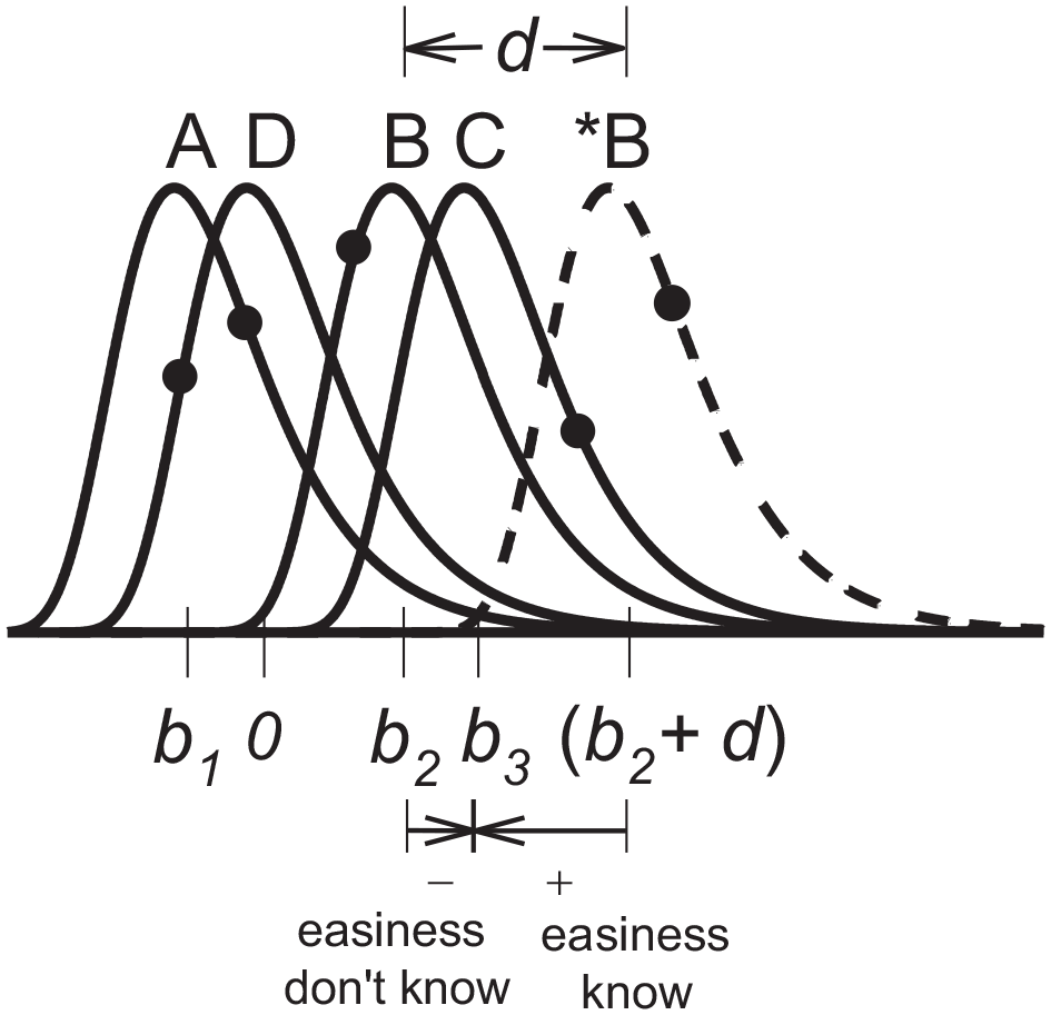
An illustration of the SDT choice model with extreme value distributions.

On any given reading, an examinee’s perceptions of the plausibility of the alternatives are realizations from each of the four distributions. The decision rule is to select the alternative with the highest perceived plausibility. For example, Figure 1 shows that, of the realizations associated with A, B, C, and D, shown as circles, the realization for Alternative C is the highest (most plausible), and so the examinee selects C, which is incorrect given that B is correct. If, on the contrary, the item is known, then it is assumed that the correct alternative is more plausible, and so the distribution is shifted to the right, as shown by the dashed distribution in Figure 1 labeled *B, where * indicates the correct answer; note that the distributions for incorrect alternatives are assumed to have the same locations. In this example, if an examinee knows the item, then the realization associated with *B is the highest of the realizations from A, *B, C, and D, and so the examinee chooses B, which is correct.

An important aspect of the above conceptualization in terms of underlying distributions is that it suggests simple measures of item discrimination and item difficulty, which are basic aspects of item response theory (IRT), and which are placed in a somewhat different perspective by SDT.

Item Discrimination

The amount that the distribution is shifted if an item is known gives a measure of item discrimination, d, as shown in Figure 1. Clearly, positive values of d are desirable, in that the item then discriminates between the states of knowing and not knowing, giving a higher probability of a correct response if the item is known. A negative value of d would mean that the correct answer is less plausible if the item is known, which suggests that the item is problematical and should be revised or dropped, as done with items that show negative (or zero) discrimination in IRT.

Item Easiness

A measure of item easiness can be defined as the distance of the distribution for the correct answer from the highest or next highest distribution. Clearly, if the other alternatives (distractors) are all much less plausible than the correct alternative, then the item is relatively “easy.” On the contrary, if one or more of the distractors is almost as plausible, or more plausible, than the correct alternative, then the item is relatively “difficult.” The easiness measure is denoted here as e_DK (easiness don’t-know) to indicate that it is easiness for an item that is not known. Note that a zero or negative value means that there is an incorrect alternative that is as plausible, or more plausible, than the correct alternative. There is also an easiness measure for when the item is known, denoted here as e_K, with $e_{K} = e_{DK} + d$ , which shows that d reflects how much easier an item is when it is known.

Figure 1 illustrates the easiness measures; the arrows show that, when the item is not known, the easiness $e_{DK} = b_{2} - b_{3}$ is negative (because b₂ is to the left of b₃), which reflects that the correct alternative B is typically less plausible than the incorrect alternative C. Although e_DK is negative, Figure 1 shows that e_K is positive, and so, when the item is known, the correct alternative B is typically more plausible than alternative C. The easiness and discrimination parameters obtained in this way are compared below to those obtained with the widely used 2PL and 3PL models, with the sign of the easiness parameter reversed to make it a difficulty parameter.

It is interesting to note that, in addition to using d to detect problematical items (i.e., zero or negative discrimination), as in IRT, an additional possibility is to use estimates of e_K to detect problematical items. In particular, a negative value of e_K means that even if the item is known, one of the incorrect alternatives is still more plausible than the correct alternative, and so it seems reasonable to suggest that items with negative estimates of e_K be dropped or revised (or at least inspected!); a benefit of the SDT approach is that the bias parameter estimates will likely indicate which alternative or alternatives are causing the problem. The use of e_K presents a new way to possibly uncover problematical items, even if the item discrimination is greater than zero; an example of this is shown in the application below.

Guessing

A common view of “guessing” is that it refers to the situation where an examinee does not know an item. Thus, the easiness parameter e_DK can also be viewed as being a measure of how easy it is to guess the correct answer when the item is not known. However, the view of “guessing” in SDT differs from that in IRT (see DeCarlo, 2020), in that guessing in SDT is not viewed as involving a separate process. Instead, examinees in SDT are viewed as always choosing the most plausible alternative (assuming the alternatives are actually read), and so the decision process is the same irrespective of whether or not an item is known; a benefit of this view is that additional item parameters for guessing are not needed (guessing depends on the examinee know/don’t know variable). In contrast, an additional item parameter for guessing is added in the 3PL model (the c parameter) and in extensions of the nominal response model (see below) because guessing is viewed as reflecting a different process.

Thus, the SDT choice model follows from three basic ideas: examinees have perceptions of the plausibility of each alternative in an MC exam; they make their decision by choosing the most plausible alternative; and the plausibility of the correct alternative differs when an item is known. As shown above, the approach yields item parameters that are analogous to those used in 2PL and 3PL models, that is, item easiness (or difficulty) and discrimination, although also with some interesting differences. In addition, the bias parameters of the SDT choice model provide measures of the relative plausibility of each of the alternatives, and so, compared with the widely used 2PL and 3PL models, the model offers more detailed information about each item, which is useful for item diagnosis and refinement. The next section shows that the above ideas lead directly to an extended SDT choice model.

The SDT Choice Model

Structural and Decision Components

As noted above, the model follows directly from earlier approaches in psychology, such as the work of Thurstone (1927) and work in SDT (Swets et al., 1961). The main components of an SDT model are a decision component, which in this case is to simply choose the most plausible alternative, and a structural component, which involves examinees’ perceptions of the alternatives and the effect of knowing or not knowing an item. Given that MC tests commonly include four or five alternatives, the model for four alternatives, as illustrated in Figure 1, is shown here; the general model immediately follows.

Let $Y_{ij}$ represent the discrete response of the ith examinee to the jth item, with values $y_{ij}$ = m for m = 1 to M, where M is the total number of alternatives; $Y_{ij}$ is treated as a nominal response variable, and so its values only indicate which alternative was chosen. Let $Ψ_{ijm}$ be a continuous latent random variable that represents the perceived plausibility of the mth alternative of the jth item to the ith examinee. Associated with the M alternatives are M dummy-coded “signal” variables, $X_{jm}$ , with a value of 1 indicating that the alternative is correct, and 0 that it is not correct. The last alternative is always used as the reference distribution (0), and M− 1 bias parameters, $b_{jm}$ , are included to allow the distributions associated with the other alternatives to have different locations (cf. DeCarlo, 2012). Let $δ_{ij}$ be a latent dichotomous variable that indicates whether item j is known by examinee i, with a value of 1 indicating yes and 0 indicating no. The structural model for the situation with four alternatives is given as follows:

\begin{matrix} {Ψ_{ij}}_{1} = {b_{j}}_{1} + d_{j} δ_{ij} {X_{j}}_{1} + {ε_{ij}}_{1}, \\ {Ψ_{ij}}_{2} = {b_{j}}_{2} + d_{j} δ_{ij} {X_{j}}_{2} + {ε_{ij}}_{2}, \\ {Ψ_{ij}}_{3} = {b_{j}}_{3} + d_{j} δ_{ij} {X_{j}}_{3} + {ε_{ij}}_{3}, \\ {Ψ_{ij}}_{4} = d_{j} δ_{ij} X_{j 4} + {ε_{ij}}_{4}, \end{matrix}

(1)

where $b_{jm}$ is the item bias, as illustrated in Figure 1, with the last bias term always set to 0; $d_{j}$ is item discrimination; and ε_ijm are random variables from a location-scale family of distributions with fixed mean (0) and fixed variance (e.g., $π^{2} / 6$ for the extreme value distribution). Equation 1 shows that the distribution locations depend on bias, $b_{jm}$ ; discrimination, $d_{j}$ ; and the state of knowing, $δ_{ij}$ ; the above generalizes the usual structural model of SDT (DeCarlo, 2010) by including a latent class component, in the same manner as for the TF SDT model and mixture SDT models (DeCarlo, 2002).

It is useful to start with a simple version of the model, in terms of SDT, without the dichotomous latent variable $δ_{ij}$ , to show the basic development. In this case, the structural model of Equation 1 simplifies to, for M-alternatives,

Ψ_{ijm} = b_{jm} + ε_{ijm} .

(2)

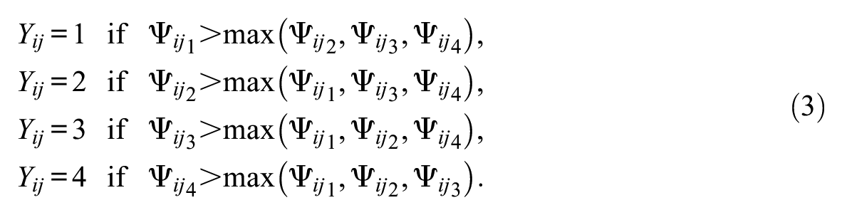
Equation 2 corresponds to the four distributions shown in Figure 1 labeled A, B, C, and D, where the bias $b_{jm}$ indicates the location of each distribution relative to the reference distribution (D). It should be obvious from Figure 1 that one can only determine the relative positions of the distributions, and so the last location, given by b_jm, is set 0. In econometrics, the above is known as a random utility model (e.g., McFadden, 1974), which was adopted from earlier ideas in mathematical psychology (McFadden, 2001), with the idea of “utility” replacing that of perception.

The decision rule is to choose alternative m if its plausibility is the largest compared with the other alternatives. Thus, for four alternatives, the decision rule is given as follows:

\begin{matrix} Y_{ij} = 1 if {Ψ_{ij}}_{1} > \max ({Ψ_{ij}}_{2}, {Ψ_{ij}}_{3}, {Ψ_{ij}}_{4}), \\ Y_{ij} = 2 if {Ψ_{ij}}_{2} > \max ({Ψ_{ij}}_{1}, {Ψ_{ij}}_{3}, {Ψ_{ij}}_{4}), \\ Y_{ij} = 3 if {Ψ_{ij}}_{3} > \max ({Ψ_{ij}}_{1}, {Ψ_{ij}}_{2}, {Ψ_{ij}}_{4}), \\ Y_{ij} = 4 if {Ψ_{ij}}_{4} > \max ({Ψ_{ij}}_{1}, {Ψ_{ij}}_{2}, {Ψ_{ij}}_{3}) . \end{matrix}

(3)

Note that it must be kept track of which option was chosen for each item, and not simply whether the choice was correct or incorrect, which loses information.

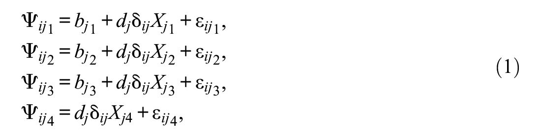
The SDT choice model follows from the structural model of Equation 2 and the decision rule of Equation 3. For example, from the decision rule, the conditional probability of a response of “1” is given as follows:

p (Y_{ij} = 1 | b_{jm}) = p [\max ({Ψ_{ij}}_{2}, {Ψ_{ij}}_{3}, {Ψ_{ij}}_{4}) < {Ψ_{ij}}_{1}] = p [({Ψ_{ij}}_{2} < {Ψ_{ij}}_{1}) \cap ({Ψ_{ij}}_{3} < {Ψ_{ij}}_{1}) \cap ({Ψ_{ij}}_{4} < {Ψ_{ij}}_{1})],

where b_jm is the vector $({b_{ij}}_{1}, {b_{ij}}_{2}, b_{ij 3}, b_{ij 4})$ in this case. Substituting the structural model of Equation 2 and rearranging terms gives the following:

p (Y_{ij} = 1 | b_{jm}) = p [({ε_{ij}}_{2} < b_{j 1} - b_{j 2} + {ε_{ij}}_{1}) \cap ({ε_{ij}}_{3} < b_{j 1} - b_{j 3} + {ε_{ij}}_{1}) \cap ({ε_{ij}}_{4} < {b_{j}}_{1} - {b_{j}}_{4} + {ε_{ij}}_{1})] .

(4)

In terms of error differences,

p (Y_{ij} = 1 | b_{jm}) = p [({ε_{ij}}_{2} - {ε_{ij}}_{1} < b_{j 1} - b_{j 2}) \cap ({ε_{ij}}_{3} - {ε_{ij}}_{1} < b_{j 1} - b_{j 3}) \cap ({ε_{ij}}_{4} - {ε_{ij}}_{1} < {b_{j}}_{1} - {b_{j}}_{4})] .

The development is the same for the other choices. One can use a joint cumulative distribution function (CDF), such as the multivariate normal, for the above probabilities, which gives a multinomial probit model. It is well known that the multinomial probit model presents computational challenges because of high-dimensional integrals when there are four or more alternatives, although some advances have been made (e.g., with maximum simulated likelihood and Bayesian estimation; see Train, 2009).

Note that, assuming that the ε_ijm of Equation 2 is independent, the terms of Equation 4 are not independent. However, the terms are conditionally independent for a given realization of ε_ij1 = e_ij₁, and so,

p (Y_{ij} = 1 | b_{jm}, {e_{ij}}_{1}) = p ({ε_{ij}}_{2} < b_{j 1} - b_{j 2} + {e_{ij}}_{1}) \times p ({ε_{ij}}_{3} < b_{j 1} - b_{j 3} + {e_{ij}}_{1}) \times p ({ε_{ij}}_{4} < {b_{j}}_{1} - {b_{j}}_{4} + {e_{ij}}_{1}) .

The unconditional probability can then be found by integrating over all values of ${ε_{ij}}_{1}$ :

p (Y_{ij} = 1 | b_{jm}) = \int_{- \infty}^{\infty} F (b_{j 1} - b_{j 2} + ε_{ij 1}) \times F (b_{j 1} - b_{j 3} + ε_{ij 1}) \times F (b_{j 1} - b_{j 4} + ε_{ij 1}) f (ε_{ij 1}) d ε_{ij 1},

where F is a CDF, f is a probability density function (PDF), and d is the derivative. The above is the model for a choice of alternative ‘1’; the same approach is used for the remaining alternatives of 2, 3, and 4 in this example, giving,

p (Y_{ij} = 1 | b_{jm}) = \int_{- \infty}^{\infty} F (b_{j 1} - b_{j 2} + ε_{ij 1}) \times F (b_{j 1} - b_{j 3} + ε_{ij 1}) \times F (b_{j 1} - b_{j 4} + ε_{ij 1}) f (ε_{ij 1}) d ε_{ij 1},

p (Y_{ij} = 1 | b_{jm}) = \int_{- \infty}^{\infty} F (b_{j 2} - b_{j 1} + ε_{ij 2}) \times F (b_{j 2} - b_{j 3} + ε_{ij 2}) \times F (b_{j 2} - b_{j 4} + ε_{ij 2}) f (ε_{ij 2}) d ε_{ij 2},

p (Y_{ij} = 1 | b_{jm}) = \int_{- \infty}^{\infty} F (b_{j 3} - b_{j 1} + ε_{ij 3}) \times F (b_{j 3} - b_{j 2} + ε_{ij 3}) \times F (b_{j 3} - b_{j 4} + ε_{ij 3}) f (ε_{ij 3}) d ε_{ij 3},

p (Y_{ij} = 1 | b_{jm}) = \int_{- \infty}^{\infty} F (b_{j 4} - b_{j 1} + ε_{ij 4}) \times F (b_{j 4} - b_{j 2} + ε_{ij 4}) \times F (b_{j 4} - b_{j 3} + ε_{ij 4}) f (ε_{ij 4}) d ε_{ij 4} .

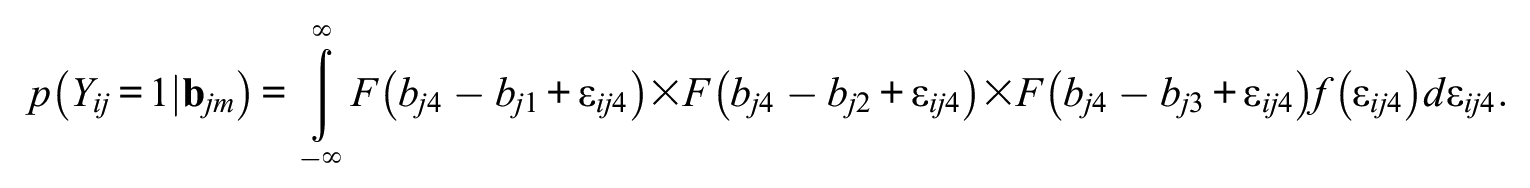
The above can be written more compactly and generally for M alternatives as follows:

p (Y_{ij} = m | b_{jm}) = \int_{- \infty}^{\infty} (Π_{\begin{matrix} k = 1 \\ k \neq m \end{matrix}}^{M} F (b_{jm} - b_{jk} + ε_{ijm})) f (ε_{ijm}) d ε_{ijm} .

(5)

Equation 5 is a general form of the basic SDT choice model; it is the same (with the addition of an alternative-specific signal variable) as the m-alternative forced choice model with bias discussed in mathematical psychology (e.g., DeCarlo, 2012) and the maximum utility model discussed in econometrics (e.g., Train, 2009).

With respect to a choice of a cumulative distribution for F and density for f, an attractive option is the extreme value Type I distribution, a distribution of smallest extremes, also known as the Gumbel distribution (Gumbel, 1958), F(x) = exp(−exp(−x)), given that it leads to simplifications. As was recognized by Luce and Suppes (1965, attributed to Holman and Marley), Yellot (1977), and McFadden (1974, Yellot and McFadden also independently showed that the extreme value solution was unique), the use of the extreme value Type I distribution in an integral such as Equation 5 leads to an MNL version of the model. Equation 5 with an extreme value distribution is given as follows:

p (Y_{ij} = m | b_{jm}) = \int_{- \infty}^{\infty} (Π_{\begin{matrix} k = 1 \\ k \neq m \end{matrix}}^{M} e^{- e^{- (b_{jm} - b_{jk} + ε_{ijm})}}) e^{- ε_{ijm}} e^{- e^{- ε_{ijm}}} d ε_{ijm} .

(6)

As shown in the Online Appendix, the above integral has a closed-form solution:

p (Y_{ij} = m | b_{jm}) = \frac{e^{b_{jm}}}{\sum_{k = 1}^{M} e^{b_{jk}}} .

(7)

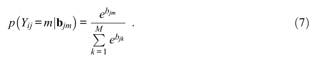
Equation 7, with bias b_jm replaced by “value,” is known in psychology as Luce’s (1959) choice model and has been the starting point for developments in psychometrics (e.g., Bock, 1972, 1997) and in econometrics (e.g., McFadden, 1974, 2001). The use of the term bias here follows from the SDT conceptualization of the situation in terms of underlying perceptual distributions, as shown above. Luce (1959) actually developed the model from axiomatic ideas, such as independence from irrelevant alternatives and transitivity, but the connection of the model to Thurstonian models was later recognized.

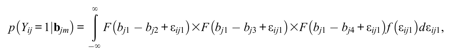
For the generalization of the SDT structural model suggested here for MC tests, Equation 1 replaces Equation 2:

Ψ_{ijm} = b_{jm} + δ_{ij} d_{j} X_{jm} + ε_{ijm},

where $δ_{ij}$ and $ε_{ijm}$ are assumed to be independent over examinees and items, δ_ij is independent of $ε_{ijm}$ , and $X_{jm}$ is a signal indicator with values of 1 for the correct alternative and 0 otherwise. The above extension simply reflects the idea that if an item is known, then the location of the distribution associated with the correct answer is shifted to the right by $d_{j}$ , that is, the item appears to be more plausible. In this case, $p (Y_{ij} = m | b_{jm})$ shown above (e.g., Equation 4) is replaced by $p (Y_{ij} = m | b_{jm}, d_{j}, X_{jm}, λ_{i})$ , with $λ_{i} = p (δ_{ij})$ . Note that the terms are conditionally independent for given values of $ε_{ijm}$ and $δ_{ij}$ , and so using the same approach as above, one must add as well as integrate to get the following:

\begin{matrix} p (Y_{ij} = m | b_{jm}, d_{j}, X_{jm}, λ_{i}) = \sum_{δ_{ij} = 0}^{1} p (δ_{ij}) p (Y_{ij} = m | b_{jm}, d_{j}, δ_{ij}, X_{jm}) \\ = \sum_{δ_{ij}} p (δ_{ij}) \int_{- \infty}^{\infty} (Π_{\begin{matrix} k = 1 \\ k \neq m \end{matrix}}^{M} F (b_{jm} - b_{jk} + δ_{ij} d_{j} (X_{jm} - X_{jk}) + ε_{ijm})) f (ε_{ijm}) d ε_{ijm} . \end{matrix}

(8)

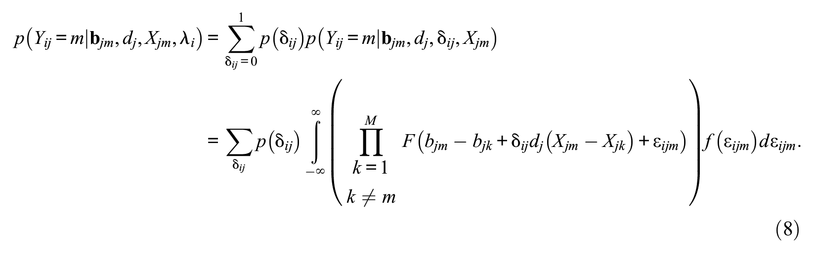
Using the extreme value distribution again gives a closed form solution, and so,

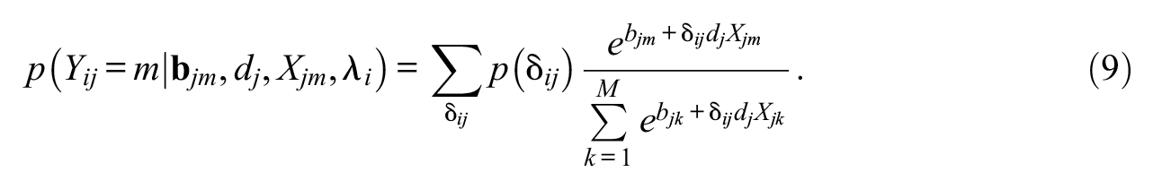
p (Y_{ij} = m | b_{jm}, d_{j}, X_{jm}, λ_{i}) = \sum_{δ_{ij}} p (δ_{ij}) \frac{e^{b_{jm} + δ_{ij} d_{j} X_{jm}}}{\sum_{k = 1}^{M} e^{b_{jk} + δ_{ij} d_{j} X_{jk}}} .

(9)

Equation 8 is a general SDT choice model for MC exams that follows from the basic ideas shown in Figure 1. Equation 9 is the version that follows with extreme value distributions. The latter model can easily be fit using maximum likelihood or posterior mode estimation (PME), with fast computational times, and so it is practical for use with large-scale exams with many items and examinees.

It is assumed that the latent variable $δ_{ij}$ is Bernoulli for a given value of $λ_{i}$ , and so, within examinees, there is a constant probability that they know the items, p( $δ_{ij}$ = 1) = $λ_{i}$ . The mixing parameter $λ_{i}$ (the latent class size) serves as an examinee variable, which is the probability that an examinee knows any given item on an exam, with $λ_{i}$ varying randomly over the i examinees; the unconditional distribution of $δ_{ij}$ depends on the choice of distribution for $λ_{i}$ (e.g., for the Beta distribution, it is Beta-binomial). Assuming a constant probability $λ_{i}$ across items for each examinee is analogous to the assumption of having parallel (or exchangeable) items in classical test theory. Note that Equation 9 can be written as follows:

p (Y_{ij} = m | b_{jm}, d_{j}, X_{jm}, λ_{i}) = λ_{i} \frac{e^{b_{jm} + d_{j} X_{jm}}}{\sum_{k = 1}^{M} e^{b_{jk} + d_{j} X_{jk}}} + (1 - λ_{i}) \frac{e^{b_{jm}}}{\sum_{k = 1}^{M} e^{b_{jk}}},

(10)

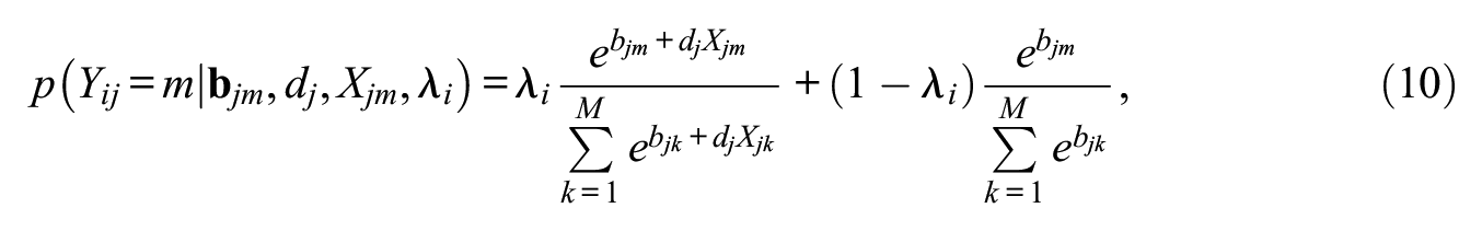
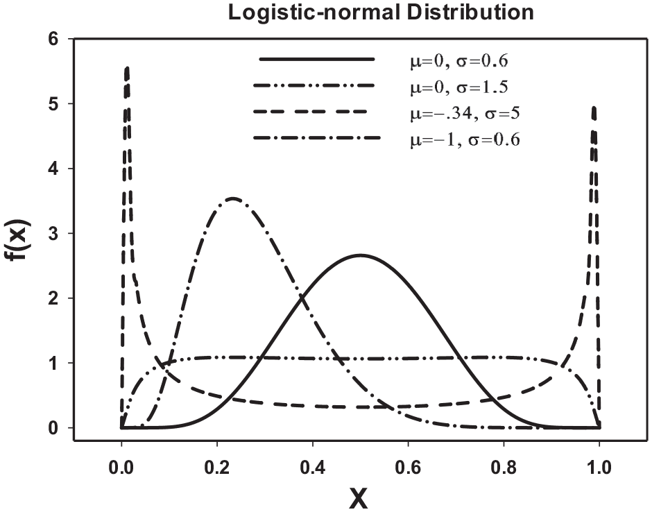
which shows that the SDT choice model is a mixture model with a random mixing parameter, $λ_{i}$ , that varies over examinees. It is important to recognize that there is mixing within examinees (cf. DeCarlo, 2002) due to the varying states of knowing or not-knowing (i.e., $δ_{ij}$ ) across items. The latent examinee variable of “knowing,” like “perception,” is viewed as being probabilistic, which recognizes the possibility, for example, of a failure to retrieve (“I know this but I can’t remember it right now”) or forgetting. Note that “knowing” has also been treated as probabilistic in earlier motivations of the 2PL and 3PL models (see DeCarlo, 2020, Figure 2, and the equation below it).

Figure 2.

Logistic-normal density for several values of μ and σ.

The random mixing parameter $λ_{i}$ is the probability that examinee i knows any given item on an exam and is analogous to θ_i in IRT. High values of $λ_{i}$ reflect a high probability of knowing any item, which is high ability in the IRT perspective, whereas a low value indicates low ability. It is also assumed that examinees are independent and that their responses are conditionally independent given $λ_{i}$ , which is the same as the assumption of conditional (local) independence of responses given $θ_{i}$ in IRT models; this allows one to compute the response pattern probabilities as the product of the individual response probabilities given by Equation 10.

To allow for a flexible distribution for $λ_{i}$ , the Beta distribution was used in earlier developments (DeCarlo, 2020; it is also a conjugate prior in Bayesian estimation) and Bayesian estimation was used; the Beta includes approximately normal, uniform, bimodal, and skewed distributions as special cases. Used here, however, is the logistic-normal distribution (Aitchison & Shen, 1980), which is similar to (though distinct from) the Beta, in that it again includes approximately normal, uniform, bimodal, and skewed distributions as special cases. The distribution arises by transforming a normal random variable, say, $θ ~ N (μ, σ)$ , with the logistic function, $e^{θ} / (1 + e^{θ})$ . The PDF of the logistic-normal is given as follows:

f (x) = \frac{1}{σ \sqrt{2 π}} \frac{1}{x (1 - x)} e^{- \frac{{(\log (\frac{x}{1 - x}) - μ)}^{2}}{2 σ^{2}}},

with 0 ≤x≤ 1. Several examples of the logistic-normal distribution, with parameter values similar to those found here for the analysis presented below (and in other analyses), are shown in Figure 2.

An advantage of the logistic-normal distribution is that it keeps the model within the framework of generalized linear models (GLMs) and so it can be fit with standard software, using maximum likelihood or PME. The logistic-normal model can be implemented by specifying a logit model (at the examinee level) for λ_i with a continuous latent predictor, say $θ_{i} ~ N (0, 1)$ :

λ_{i} = p (δ_{ij} = 1) = \frac{e^{μ + σ θ_{i}}}{1 + e^{μ + σ θ_{i}}},

(11)

and so $λ_{i}$ has a logistic-normal distribution. Note that Equation 11 contains a normal latent examinee variable, θ_i, which is analogous to $θ_{i}$ in IRT models, with the difference that the SDT choice model has two additional (examinee level) parameters, μ and $σ$ , which determine the shape of the $λ_{i}$ distribution (see Figure 2). Using Equation 11, the probability of Equation 10 not conditional on $λ_{i}$ can be found using Gaussian quadrature for $θ_{i}$ in the usual manner, and so the model can be implemented in software for extended MNL models (and choice models), such as Latent Gold (LG; Vermunt & Magidson, 2016). The Online Appendix provides an LG program to fit the model; parameter recovery with LG is also examined in simulations.

Note that in the SDT choice model, the latent dichotomous variable $δ_{ij}$ varies within examinees (over items) and across examinees. The model differs from other generalizations of the MNL model in econometrics, such as the mixed MNL model, the latent class MNL model, and mixed-mixed MNL models (e.g., Hensher et al., 2015; Train, 2009) in that in the current context, those models allow the parameters $b_{jm}$ and $d_{j}$ to be random (continuous or discrete) across examinees, whereas $d_{j}$ of the SDT choice model varies within examinees (across items) because of $δ_{ij}$ . Another view is that the just noted MNL models do not allow for random mixing, but instead segment the examinees into different latent classes, and so the mixing parameter is fixed.

Equation 10 can be viewed, statistically, as an extended latent class MNL choice model with random mixing (random class sizes) and is similar to a grade-of-membership (GoM; Erosheva, 2002) extension. From the GoM perspective, $λ_{i}$ can be viewed as an examinee’s distance from, or grade-of-membership in, the extremal states of knowing none of the items versus knowing all of the items; see DeCarlo (2020) for further discussion and comparisons.

Bock’s Nominal Response Model

The SDT choice model is related to, but also differs from, approaches to MC items previously developed in psychometrics. It is closely related to Bock’s (1972, 1997) nominal response model, and so some similarities and differences are briefly discussed in this section.

The nominal response model generalizes Luce’s choice model by replacing “value” (bias in Equation 7) with item trace functions from IRT, that is, $b_{jm} + a_{jm} θ_{i}$ , with $θ ~ N (0, 1)$ and with constraints on the item parameters for identification, typically $\sum_{m = 1}^{M} b_{jm} = 0$ and $\sum_{m = 1}^{M} a_{jm} = 0$ . Bock (1972) noted that a psychological interpretation of the model is that “Each alternative of item j is assumed to give rise to a quantitative ‘response tendency’ in a given subject” (p. 30), which is similar to, but also differs from, the SDT view, in that SDT replaces “response tendency” with perception. The interpretation differs in that $b_{jm}$ in SDT is viewed as reflecting the relative plausibility of the alternatives, and d_j indicates how well the item discriminates between states of knowing and not knowing. Nevertheless, estimates of $b_{jm}$ for the SDT choice model are similar to those obtained with the nominal response model, with respect to ranking the plausibility of the alternatives, as shown below.

An important difference between the models is that the nominal response model includes discrimination parameters, $a_{jm}$ , for all of the alternatives because it assumes that there are different trace lines for each alternative, whereas the discrimination parameter $d_{j}$ in the SDT model does not vary across the alternatives, and so the nominal model has J× (M− 1) discrimination parameters, whereas the SDT model has only J discrimination parameters. The interpretation of discrimination in SDT as the amount that a plausibility distribution is shifted for the correct alternative when an item is known suggests only one discrimination parameter per item, given that discrimination only applies to the correct alternative. Besides the simpler conceptualization, the reduction in parameters offered by the SDT approach also simplifies estimation and interpretation, as shown in the application.

A common criticism of the nominal response model (e.g., Nering & Ostini, 2010) is that it does not deal with guessing, like the 3PL model. To address this, Thissen and Steinberg (1984) generalized Bock’s nominal response model by assuming that there is a category of “don’t know” examinees. Using this idea leads to an extended nominal model which adds a latent proportion of examinees who do not know an item, sometimes denoted as d_h, which adds an additional J× (M−1) guessing parameters. Thissen and Steinberg (1997) recognized an overparameterization problem: “The focus of the problem is the large number of parameters involved . . .” (pp. 57–58) and “The solution to the problem is obviously to reduce the number of parameters; but it is not clear, a priori, which parameters are needed to fit which items” (p. 58). In contrast, additional guessing parameters are not needed in SDT because guessing is viewed as involving the same decision process—choose the most plausible alternative—which is an important advantage. The SDT approach provides, a priori, a way of reducing the number of parameters and provides a conceptual basis for what is restricted and why, with a straightforward interpretation.

An Application: SAT12 Data

The data are given in the R package MIRT as an example application of the nominal response model (Chalmers, 2012) and consist of 32 SAT items with five alternatives per item and 600 examinees. For the 32 × 600 = 19,200 observations, 69 were missing the choice response and were not included, leaving 19,131 observations.

Parameter Estimates

The SDT choice model and nominal response model were both fit using LG; note that for the SDT model, the discrimination parameter $d_{j}$ and σ of Equation 11 were restricted to be positive. Although maximum likelihood estimation could be used, it is well known that there are frequently estimation problems in latent class models, such as boundary problems (e.g., DeCarlo, 2011, 2019; Vermunt & Magidson, 2016), and so PME was used (with Bayes constants of 1); PME smooths parameter estimates away from boundaries and helps to deal with estimation problems; it has previously been used for latent class signal detection models and cognitive diagnostic models (for references, see DeCarlo, 2019).

For the SDT model, for each item, there are four estimates of $b_{jm}$ (with b_j₅ = 0) and one estimate of discrimination, $d_{j}$ . The item parameter estimates are shown in Table 1, along with the derived item easiness measures e_DK and e_K. Note that the bias parameters $b_{jm}$ only order the alternatives within items, and not across items, because of the arbitrary choice of the last alternative as the zero point. The parameters e_DK, e_K, and d_j, on the contrary, are based on differences, and so they are not affected by the choice of zero point and can be compared across items.

Table 1.

Parameter Estimates for the SDT Choice Model, SAT12 Data, Five Alternatives, N =600, b_j₅ = 0.

Logistic-normal estimates: $\hat{μ}$ = −0.34 (0.11), $\hat{σ}$ = 5.00 (1.40)
Item	b_j ₁	SE	b_j ₂	SE	b_j ₃	SE	b_j ₄	SE	d_j	SE	e _DK	e _K
1	*2.08	(0.42)	2.72	(0.36)	3.00	(0.36)	2.85	(0.36)	1.80	(0.31)	−0.92	0.88
2	0.51	(0.15)	−1.77	(0.30)	−0.59	(0.19)	*0.24	(0.19)	3.48	(0.47)	−0.27	3.21
3	0.81	(0.27)	0.91	(0.27)	1.26	(0.27)	0.29	(0.29)	2.35	(0.34)	−1.26	1.09
4	0.25	(0.15)	*0.37	(0.19)	0.14	(0.16)	0.29	(0.15)	1.46	(0.26)	0.08	1.54
5	0.66	(0.23)	1.09	(0.21)	*1.72	(0.22)	0.66	(0.23)	2.18	(0.31)	0.63	2.81
6	*−1.10	(0.39)	1.68	(0.14)	−0.02	(0.18)	−0.92	(0.23)	2.36	(0.44)	−2.78	−0.42
7	0.41	(0.41)	*3.10	(0.33)	−0.91	(0.59)	2.43	(0.33)	2.38	(0.43)	0.67	3.05
8	*−0.48	(0.27)	0.43	(0.14)	0.44	(0.14)	0.63	(0.14)	1.57	(0.34)	−1.11	0.46
9	2.28	(0.52)	0.41	(0.65)	*4.46	(0.51)	1.61	(0.55)	1.27	(0.43)	2.18	3.45
10	*−0.24	(0.21)	0.25	(0.13)	−0.01	(0.14)	−1.77	(0.26)	2.38	(0.30)	−0.49	1.89
11	0.69	(1.22)	*5.76	(1.00)	1.61	(1.09)	0.69	(1.22)	6.32	(8.92)	4.15	10.47
12	−1.05	(0.18)	−0.92	(0.17)	0.06	(0.13)	*0.54	(0.16)	0.37	(0.24)	0.48	0.85
13	1.01	(0.24)	*1.95	(0.23)	0.56	(0.26)	1.08	(0.24)	2.51	(0.37)	0.87	3.38
14	*1.05	(0.16)	−1.48	(0.28)	−0.07	(0.17)	−1.68	(0.30)	2.47	(0.41)	1.05	3.52
15	−2.42	(0.24)	−1.85	(0.19)	−1.88	(0.19)	−2.75	(0.27)	2.90	(0.60)	1.85	4.75
16	−1.02	(0.18)	−0.62	(0.16)	*−0.04	(0.18)	0.10	(0.13)	1.65	(0.27)	−0.14	1.51
17	−0.47	(0.57)	−0.98	(0.68)	−0.29	(0.54)	*3.70	(0.37)	2.85	(1.24)	3.70	6.55
18	0.76	(0.13)	−1.45	(0.25)	0.15	(0.15)	*−1.43	(0.45)	3.97	(0.53)	−2.19	1.78
19	*3.20	(0.43)	1.67	(0.44)	3.58	(0.41)	1.10	(0.47)	1.92	(0.28)	−0.38	1.54
20	0.56	(0.63)	−1.38	(1.12)	2.76	(0.52)	*4.14	(0.51)	4.97	(2.80)	1.38	6.35
21	1.45	(0.42)	−0.34	(0.59)	*3.94	(0.40)	0.13	(0.52)	1.30	(0.52)	2.49	3.79
22	0.64	(0.41)	−1.10	(0.67)	*3.46	(0.34)	0.11	(0.46)	7.68	(9.25)	2.82	10.50
23	1.21	(0.16)	0.71	(0.17)	0.39	(0.18)	*0.47	(0.23)	1.57	(0.27)	−0.74	0.83
24	*1.94	(0.22)	1.28	(0.22)	−0.08	(0.28)	−0.73	(0.34)	2.99	(0.52)	0.66	3.65
25	0.53	(0.14)	0.18	(0.15)	0.05	(0.21)	*−0.78	(0.19)	1.84	(0.28)	−0.48	1.36
26	−1.54	(0.36)	0.89	(0.23)	−1.13	(0.32)	1.03	(0.23)	3.53	(0.40)	−1.03	2.50
27	*3.70	(0.42)	2.23	(0.43)	0.15	(0.56)	0.69	(0.50)	4.51	(1.90)	1.47	5.98
28	0.80	(0.26)	−1.30	(0.46)	1.62	(0.26)	*2.22	(0.22)	2.47	(0.31)	−0.60	1.87
29	*0.58	(0.25)	1.49	(0.18)	1.12	(0.18)	0.24	(0.21)	2.01	(0.30)	−0.91	1.10
30	−0.66	(0.1)7	−0.97	(0.18)	−1.00	(0.18)	−0.46	(0.16)	0.89	(0.24)	0.46	1.35
31	0.25	(0.23)	−1.07	(0.33)	−1.61	(0.41)	*1.84	(0.19)	7.39	(8.66)	1.59	8.98
32	−0.20	(0.21)	0.18	(0.20)	1.06	(0.19)	−0.71	(0.23)	0.12	(0.30)	−1.06	−0.94

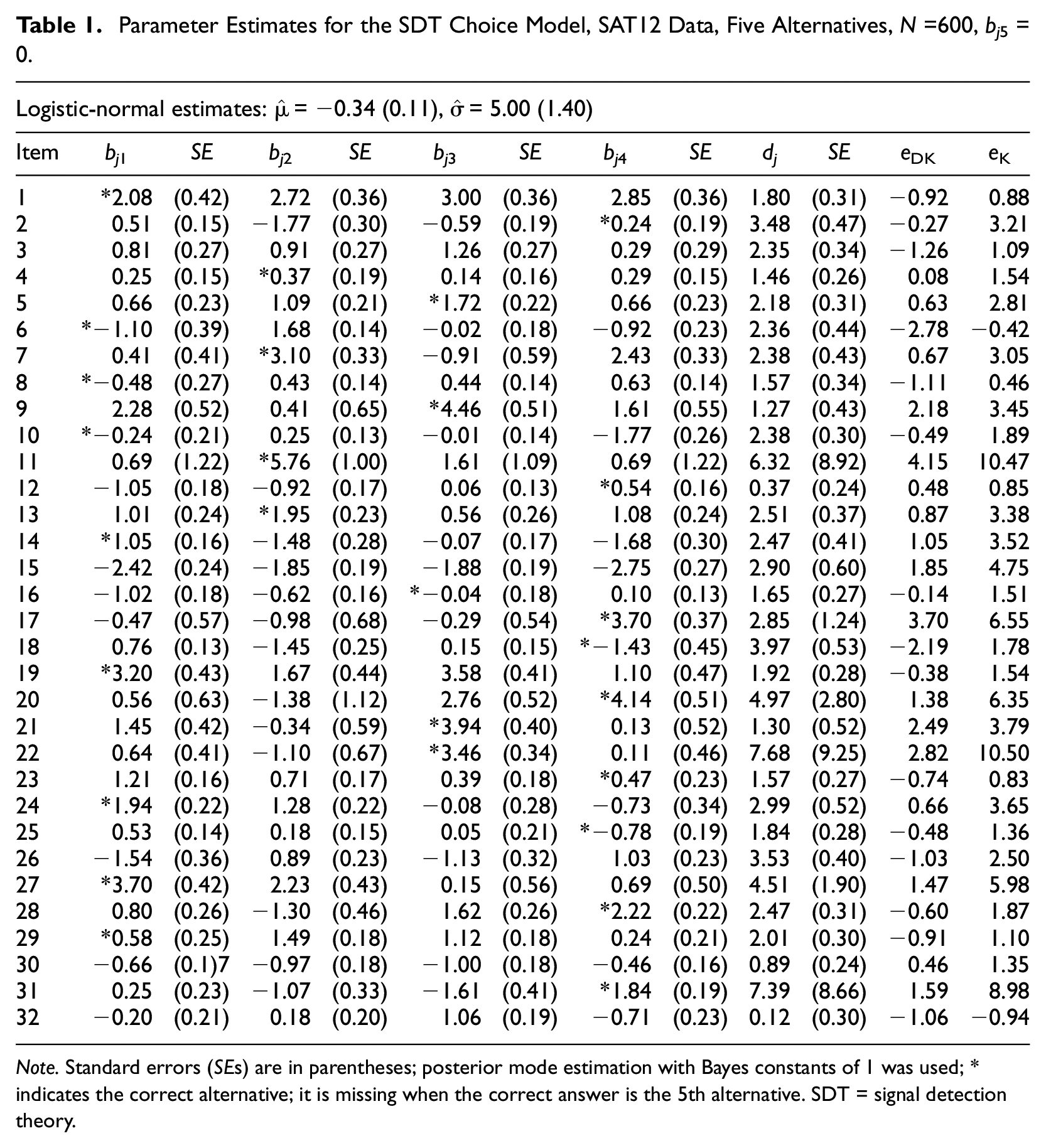
Note. Standard errors (SEs) are in parentheses; posterior mode estimation with Bayes constants of 1 was used; * indicates the correct alternative; it is missing when the correct answer is the 5th alternative. SDT = signal detection theory.

The estimates of $b_{jm}$ in Table 1 order the alternatives (within items) in terms of their relative plausibility. For example, for Item 17; the estimates of e_DK in Table 1 show that of the 32 items, Item 17 is the second easiest item if it is not known ( ${\hat{e}}_{DK}$ = 3.7) with estimates of bias of (−0.47, −0.98, −0.29, *3.70, 0.00) for Alternatives 1, 2, 3, 4, and 5, with “*” indicating the correct answer. This shows that even if the item is not known, the distractors are all considerably less plausible (<0) than the correct alternative (3.7), and so the item is easy. The discrimination parameter of 2.85 indicates how much easiness is increased if the item is known (3.7 + 2.85 = 6.55). Note that the SDT approach also suggests what to do with respect to manipulating item easiness—if one wishes to revise Item 17 to make it more difficult, then more plausible distractors are needed, particularly with respect to Alternatives 1, 2, and 3, and so the SDT model provides valuable information with respect to understanding the items and how to revise them.

Nearly half of the 32 estimates of $e_{DK}$ in Table 1 are negative, which indicates that if the item is not known, then at least one alternative is more plausible than the correct answer; for the remaining items, the correct answer is the most plausible. In contrast, all of the estimates of $e_{K}$ (easiness if the item is known) are positive, with two notable exceptions, Items 6 and 32. As noted above, negative estimates suggest that the items might be problematical, in that one of the alternatives might be more plausible than the correct alternative, even if the item is known. For Item 32, Table 1 shows that if the item is not known, Alternative 3 is clearly more plausible than the rest of the alternatives, including the correct answer (Alternative 5); the bias estimates are (−0.20, 0.18, 1.06, −0.71, *0.00) and so ${\hat{e}}_{DK}$ is −1.06. The table shows that the problem with negative $e_{K}$ arises because the discrimination parameter is small (0.12) and so ê_K = −1.06 + 0.12 = −0.94, which is still negative, and so an incorrect answer (Alternative 3) is still more plausible than the correct answer (Alternative 5).

A problem with Item 32 has previously been noted in the MIRT manual (Chalmers, 2012): “careful analysis using the nominal response model suggests that the scoring key for Item 32 may be incorrect, and should be changed from 5 to 3” (p. 158). The problem with Item 32 is immediately apparent in the SDT analysis, given that a negative estimate of e_K appears in Table 1.

The SDT analysis, however, also suggests that another item might be problematical, Item 6, because Table 1 shows that ${\hat{e}}_{K}$ is negative (−0.42); to my knowledge, a problem with Item 6 has not previously been noted. Table 1 shows that the estimates of bias when the item is not known are (*−1.10, 1.68, −0.02, −0.92, 0.00), and so the correct answer, Alternative 1, is the least plausible of the alternatives (−1.10), whereas Alternative 2 is the most plausible (1.68). However, for those who know the item, the plausibility of Alternative 1 is −1.10 + 2.36 = 1.26, and so Alternative 1 is still less plausible (1.26) than Alternative 2 (1.68) even if the item is known (and so ${\hat{e}}_{K}$ = 1.26 − 1.68 = −0.42), which suggests a problem. It is not known whether this reflects a problem with the scoring key or a problem with the item, but the important aspect is that the SDT analysis immediately calls attention to this sort of problem, which is not the case for the nominal response model, as shown below. Furthermore, evidence as to the validity of the potential problem as detected by SDT could be obtained by inspecting the actual item and alternatives (not available in this case).

What about simply inspecting response proportions for each alternative? The potential problem with that approach is that, according to the mixture SDT model, the response proportion for the correct alternative is actually a mixture of proportions for those who know and those who don’t know the item and so ignoring this can lead to incorrect conclusions. Item 8 provides a nice example. The proportions for this item are (*0.20, 0.21, 0.21, 0.25, 0.13), and so Alternative 4 is the most often selected (0.25) even though Alternative 1 is the correct answer. Does this mean that the item is problematical? A fit of the SDT choice model readily answers this question. If the item is not known, then from Table 1, the bias estimates are (*−0.48, 0.43, 0.44, 0.63, 0.00), which shows not only that Alternative 4 has the highest plausibility (0.63) but also that the correct answer of Alternative 1 has the lowest plausibility (−0.48) compared with the remaining three alternatives. If the item is known, on the contrary, then the plausibility for Alternative 1 is −0.48 + 1.57 = 1.09, and so Alternative 1 is now the most plausible (and ${\hat{e}}_{K}$ is positive, 1.09 − 0.63 = 0.46). Thus, analysis with the SDT choice model does not tag the item as being problematical, whereas this is not clear from an inspection of response proportions.

With respect to discrimination (d_j), Table 1 shows that the estimates are all greater than 0; however, Items 12 and 32 have small, insignificant estimates of 0.37 and 0.12, respectively (this is also true for the 2PL model, but not for the 3PL model). Estimates of discrimination for Items 11, 22, and 31 are large (6.32, 7.68, 7.39) with large standard errors (8.92, 9.25, 8.66); larger standard errors often occur for large values of the parameters (d_j > 6 is high discrimination) and so there is weak information about some of the estimates of discrimination.

The estimates of $μ$ and $σ$ for the logistic-normal distribution are −0.34 (0.11) and 5.00 (1.40), respectively, and so the distribution of $λ_{i}$ is bimodal (with a higher lower mode), see Figure 2, as was also found for lambda for TF data (DeCarlo, 2020). Thus, examinees tend to be clustered close to the (extremal) states of knowing all or none of the items. However, compared with a simple latent class version of the model, with examinees simply in one of two extremal states (knowing all of the items vs. knowing none of the items), the SDT choice model has better relative fit (there are also convergence problems for the latent class model).

2PL and 3PL Models

Given that the SDT choice model provides estimates of discrimination and easiness, it is of interest to compare them with those obtained using the 2PL and 3PL models (fit here using PROC IRT of SAS). As found earlier, the results for the SDT choice model are similar to those found for the 2PL model (DeCarlo, 2020). The Spearman correlations of −ê_DK with estimates of b_j for the 2PL and 3PL models are .86 (2PL) and .84 (3PL); the correlations of −ê_K with estimates of b_j are .94 (2PL) and .92 (3PL). The Spearman correlations of estimates of d_j with estimates of a_j are .97 (2PL) and .04 (3PL). Thus, as found earlier, estimates of difficulty and discrimination from the SDT model are correlated with those found for the 2PL model; however, discrimination differs for the 3PL model. This also holds for a comparison of the 2PL and 3PL models—the Spearman correlation of the estimates of difficulty ( $b_{j}$ ) across the 2PL and 3PL models is .99; however, the correlation of discrimination estimates (a_j) is only .10 (cf. DeCarlo, 2020). This shows that including a guessing parameter causes marked differences in estimates of discrimination across 2PL and 3PL models, and so the results with respect to discrimination depend on the choice of IRT model.

Estimates of the guessing parameter for the 3PL model range from 0.00 to 0.48 and is 0.00 (or 0.02) for nine of the 32 items. This strongly suggests that the parameter does not reflect a process of guessing—if one is randomly choosing among five alternatives, then the choice should be correct about 20% of the time, and not 0% in many cases (or 48%); this problem does not arise for the SDT model because of the different conceptualization of guessing.

With respect to detecting the possibly problematic Items 6 and 32, discussed above, neither the 2PL nor 3PL parameter estimates suggest a problem for Item 6; estimates and standard errors for the 2PL are ${\hat{b}}_{j}$ = 1.78 (0.20) and ${\hat{a}}_{j}$ = 1.15 (0.15), and for 3PL, ${\hat{b}}_{j}$ = 1.52 (0.12), ${\hat{a}}_{j}$ = 2.84 (0.72), and ${\hat{c}}_{j}$ = 0.07 (0.02), and so a potentially problematical item is completely missed. For Item 32, estimates and standard errors for the 2PL model are ${\hat{b}}_{j}$ = 14.78 (14.81) and ${\hat{a}}_{j}$ = 0.12 (0.12), which suggest estimation problems, and for 3PL model, ${\hat{b}}_{j}$ = 2.50 (0.36), ${\hat{a}}_{j}$ = 3.07 (1.65), and ${\hat{c}}_{j}$ = 0.15 (0.02).

It is also of interest to compare the predictions of examinee ability across the models. Posterior estimates of θ_i for the 2PL model and 3PL models, and the proportion correct (PC), were highly correlated with posterior estimates of $λ_{i}$ (or $θ_{i}$ ) for the SDT model, with Spearman correlations of .99 (2PL), .97 (3PL), and .98 (PC). Thus, the SDT choice model rank orders examinees in the same way as the 2PL/3PL models, as well as the simple PC.

Note that information criteria, such as the Bayesian information criterion (BIC; Schwarz, 1978) or Akaike’s information criterion (AIC; Akaike, 1974), cannot be used to compare relative fit of the SDT choice model to the 2PL or 3PL models because the models use different data—the choice model is fit to the original 1 to 5 responses—whereas the 2PL and 3PL models are fit to responses recoded as 0 or 1 for incorrect or correct, and so the log-likelihoods are not comparable. Bock’s nominal response model, however, applies to the original 1 to 5 responses, like the SDT choice model, and so BIC and AIC can be compared across the models, as done next.

Bock’s Nominal Response Model

For Bock’s nominal response model, there are eight parameters per item, four $b_{jm}$ and four $a_{jm}$ , giving a total of 256 parameters for 32 items, in contrast to the 162 parameters for the SDT model (four $b_{jm}$ and one $d_{j}$ per item, plus two parameters for the logistic-normal). The parameter estimates for the nominal model, with the usual sum-to-zero constraints, are shown in Table A1 in the Online Appendix (again using PME and Bayes constants of 1 in LG). The table shows that there is an estimation problem for Item 11, given that both the $b_{jm}$ and $a_{jm}$ estimates are large with large standard errors, and so there is weak information for this item.

Information criteria for the SDT choice and nominal response model, respectively, are BIC = 40,035.7 and 40,376.3, which favors the SDT model, and AIC = 38,762.5 and 38,363.5, which favors the nominal model. This type of pattern is often found with these criteria—BIC tends to favor simpler models (i.e., fewer parameters, as in the choice model, because BIC has a larger penalty for parameters), whereas AIC tends to favor more complex models (such as the nominal response model). One could argue for the SDT choice model on the basis of parsimony (i.e., favor the BIC); however, the important question is not relative statistical fit, but rather is whether anything is gained by introducing 128 discrimination parameters in the nominal response model, as compared with 32 in the SDT choice model.

Table A1 shows that estimates of $b_{jm}$ from the nominal response model order the alternatives in a similar way as the $b_{jm}$ of the mixture SDT choice model (Table 1), with the rank order being the same for nine of the 32 items, and the rest typically differing by only one category. Table A1 also shows that for the nominal model with five estimates of discrimination $a_{jm}$ per item (with a sum to zero constraint), discrimination is typically largest for the correct alternative, except for Item 32 (and Item 12, where there is in essence a tie); discrimination is also always positive for the correct alternative.

As discussed above, the SDT analysis tagged Item 32 as being problematical. Table A1 shows that for the nominal model, the estimate of $b_{jm}$ for (incorrect) Alternative 3 (0.99) is largest among the alternatives, and so is the estimate of discrimination a_jm (0.40). On the contrary, for Alternative 5, which is reported as the correct answer, the estimates of $b_{jm}$ and $a_{jm}$ are both smaller (0.01 and 0.29 respectively). This is likely why it was speculated that Alternative 3 was in fact the correct answer and not Alternative 5—both $b_{jm}$ and $a_{jm}$ are largest for Alternative 3 of Item 32. In this case, the conclusion from the nominal response model agrees with that from the SDT model as well as a simple analysis of response proportions.

This is not the case, however, for Item 6. Item 6 is tagged as being problematical by the SDT analysis because of the negative estimate of $e_{K}$ (−0.42, Table 1), which suggests that, even if the item is known, an incorrect alternative (Alternative 2) is more plausible than the correct alternative (Alternative 1). For the nominal response model, on the contrary, the estimate of $b_{jm}$ is largest (1.56) for the incorrect alternative of “2” but is negative (−0.11) for the correct alternative of “1.” The estimate of discrimination $a_{jm}$ has the opposite pattern and is large and positive (0.84) for the correct alternative of “1” but is negative (−0.24) for Alternative 2. Thus, the nominal results differ across $b_{jm}$ and $a_{jm}$ , in that an incorrect alternative has the largest $b_{jm}$ , but negative $a_{jm}$ , whereas the correct alternative has the largest $a_{jm}$ , but a small $b_{jm}$ , and so the results are not clear, which is likely why Item 6 has not previously been tagged as being problematical in a nominal response analysis, in contrast to the SDT analysis.

A different pattern across estimates of $b_{jm}$ and $a_{jm}$ also appears for Item 8 in Table A1—the correct alternative has a smaller estimate of $b_{jm}$ than an incorrect alternative, and a negative estimate of discrimination $a_{jm}$ , and so it is again not clear as to what to conclude from the nominal response analysis. The response proportions (given above) also show that an incorrect answer is the most frequently chosen, so it is still not clear what to conclude. However, as discussed above, the SDT analysis does not tag Item 8 as being problematical because the estimate of e_K is positive, that is, the correct answer is the most plausible if the item is known, and so the interpretation in terms of SDT is simple and clear; it also again suggests that one could obtain evidence of validity by actually inspecting the item and alternatives. The results for Items 6 and 8 suggest that the 128 discrimination parameters in the nominal response model might be complicating the interpretation of the results rather than clarifying them.

Spearman correlations of estimates of $λ_{i}$ (or $θ_{i}$ ) for the SDT model with estimates of $θ_{i}$ for the 2PL, 3PL, nominal models, and PC, respectively, are .99, .97, .97, and .98. Thus, all three IRT models and the PC appear to offer essentially the same ranking of examinees as the SDT choice model.

Discussion

A signal detection model for multiple choice exams is presented. The approach views examinees as choosing, for each item, the alternative that is perceived as being the most plausible. It is also assumed that knowing an item shifts the perception in the direction of greater plausibility for the correct alternative. These assumptions together lead to a mixture SDT choice model. The choice model offers information about the items that is comparable with that offered by the 2PL model, in terms of discrimination and difficulty, but it also offers important information about the plausibility of the distractors. This in turn can reveal possible problems with alternatives in an item. For example, an application shows that the SDT model detects possibly problematical items that are missed by an analysis using the nominal response model, the 2PL or 3PL models, or simple inspection of response proportions. An important aspect of the SDT approach is that it also suggests how to obtain evidence of validity—if one could inspect the actual item and its’ alternatives in the above examples, then that would help to determine whether the problems suggested above by the SDT analysis have validity. Another advantage is that the interpretation of the results in terms of SDT is simple and straightforward, which is important for practitioners. The benefit of adding a large number of discrimination parameters, as in the nominal response model, was called into question. The mixture SDT choice model provides a simple unified model that can replace the 2PL, 3PL, and nominal response models, or a simple analysis of proportions.

The most basic (and strictest) version of the SDT model is presented here; there are of course many possible extensions and issues for further examination. For example, a version of the model with random discrimination parameters across examinees was examined in DeCarlo (2020). Another option is to use response times to obtain collateral information to improve estimation (van der Linden et al., 2010). Yet, another interesting possibility is to use covariates to allow the random mixture parameter $λ_{i}$ to vary across items or groups of items (for multidimensional items), or to see whether the mixing parameter is related to various examinee variables or response times.

Supplemental Material

sj-pdf-1-apm-10.1177_01466216211014599 – Supplemental material for A Signal Detection Model for Multiple-Choice Exams

Supplemental material, sj-pdf-1-apm-10.1177_01466216211014599 for A Signal Detection Model for Multiple-Choice Exams by Lawrence T. DeCarlo in Applied Psychological Measurement

Footnotes

Declaration of Conflicting Interests

The author(s) declared no potential conflicts of interest with respect to the research, authorship, and/or publication of this article.

Funding

The author(s) received no financial support for the research, authorship, and/or publication of this article.

ORCID iD

Lawrence T. DeCarlo

Supplemental Material

Supplementary material is available for this article online.

References

Aitchison

Shen

S. M.

(1980). Logistic-normal distributions: Some properties and uses. Biometrika, 67, 261–272.

Akaike

(1974). A new look at the statistical model identification. IEEE Transactions on Automatic Control, 19, 716–723.

Birnbaum

(1968). Some latent trait models. In Lord

F. M.

Novick

M. R.

(Eds.), Statistical theories of mental test scores (pp. 397–424). Addison-Wesley.

Bock

R. D.

(1972). Estimating item parameters and latent ability when responses are scored in two or more nominal categories. Psychometrika, 37, 29–51.

Bock

R. D.

(1997). The nominal categories model. In van der Linden

W. J.

Hambleton

R. K.

(Eds.), Handbook of modern item response theory (pp. 33–49). Springer.

Chalmers

R. P.

(2012). MIRT: A multidimensional item response theory package for the R environment. Journal of Statistical Software, 48, 1–29. https://doi.org/10.18637/jss.v048.i06

de Ayala

R. J.

(2009). The theory and practice of item response theory. Guilford Press.

DeCarlo

L. T.

(2002). Signal detection theory with finite mixture distributions: Theoretical developments with applications to recognition memory. Psychological Review, 109, 710–721.

DeCarlo

L. T.

(2010). On the statistical and theoretical basis of signal detection theory and extensions: Unequal variance, random coefficient, and mixture models. Journal of Mathematical Psychology, 54, 304–313.

10.

DeCarlo

L. T.

(2011). On the analysis of fraction subtraction data: The DINA model, classification, latent class sizes, and the Q-matrix. Applied Psychological Measurement, 35, 8–26.

11.

DeCarlo

L. T.

(2012). On a signal detection approach to m-alternative forced choice with bias, with maximum likelihood and Bayesian approaches to estimation. Journal of Mathematical Psychology, 56, 196–207.

12.

DeCarlo

L. T.

(2019). Insights from reparameterized DINA and beyond. In von Davier

Lee

Y.-S.

(Eds.), Handbook of diagnostic classification models (pp. 223–243). Springer.

13.

DeCarlo

L. T.

(2020). An item response model for true-false exams based on signal detection theory. Applied Psychological Measurement, 44, 215–229.

14.

Erosheva

E. A.

(2002). Grade of membership and latent structure models with application to disability survey data [Doctoral dissertation]. Carnegie Mellon University.

15.

Fechner

(1966). Elements of psychophysics. Holt, Rinehart and Winston. (Original work published 1860)

16.

Green

D. M.

Swets

J. A.

(1988). Signal detection theory and psychophysics. Peninsula Publishing. (Reprinted from 1966)

17.

Gumbel

E. J.

(1958). Statistics of extremes. Columbia University Press.

18.

Hensher

D. A.

Roxe

J. M.

Greene

W. H.

(2015). Applied Choice Analysis (2nd ed.). Cambridge University Press.

19.

Luce

R. D.

(1959). Individual choice behavior: A theoretical analysis. John Wiley.

20.

Luce

R. D.

Suppes

(1965). Preference, utility, and subjective probability. In Luce

R. D.

Bush

R. R.

Galanter

(Eds.), Handbook of mathematical psychology (Vol. 3, pp. 249–410). John Wiley.

21.

Macmillan

N. A.

Creelman

C. D.

(2005). Detection theory: A user’s guide (2nd ed.). Lawrence Erlbaum.

22.

McFadden

(1974). Conditional logit analysis of qualitative choice behavior. In Zarembka

(Ed.), Frontiers in econometrics (pp. 105–142). John Wiley.

23.

McFadden

(2001). Economic choices. The American Economic Review, 91, 351–378.

24.

Nering

M. L.

Ostini

(2010). Handbook of polytomous item response theory models. Routledge.

25.

Schwarz

(1978). Estimating the dimension of a model. Annals of Statistics, 6, 461–464.

26.

Swets

J. A.

Tanner

W. P.

Jr. Birdsall

T. G.

(1961). Decision processes in perception. Psychological Review, 68, 301–340.

27.

Thissen

Steinberg

(1984). A response model for multiple choice items. Psychometrika, 49, 501–519.

28.

Thissen

Steinberg

(1997). A response model for multiple-choice items. In van der Linden

W. J.

Hambleton

R. K.

(Eds.), Handbook of modern item response theory (pp. 51–65). Springer.

29.

Thurstone

L. L.

(1927). A law of comparative judgment. Psychological Review, 34, 273–286.

30.

Train

K. E.

(2009). Discrete choice methods with simulation (2nd ed.). Cambridge University Press.

31.

van der Linden

W. J.

Klein Entink

R. H.

Fox

J.-P.

(2010). IRT parameter estimation with response times as collateral information. Applied Psychological Measurement, 34, 327–347.

32.

Vermunt

J. K.

Magidson

(2016). Technical guide for LatentGOLD 5.1: Basic, advanced, and syntax. Statistical Innovations.

33.

Wickens

T. D.

(2002). Elementary signal detection theory. Oxford University Press.

34.

Yellot

J. I.

Jr. (1977). The relationship between Luce’s choice axiom, Thurstone’s theory of comparative judgment, and the double exponential distribution. Journal of Mathematical Psychology, 15, 109–144.

Supplementary Material

Please find the following supplemental material available below.

For Open Access articles published under a Creative Commons License, all supplemental material carries the same license as the article it is associated with.

For non-Open Access articles published, all supplemental material carries a non-exclusive license, and permission requests for re-use of supplemental material or any part of supplemental material shall be sent directly to the copyright owner as specified in the copyright notice associated with the article.

0.00 MB

0.63 MB