Flexible Item Response Models for Count Data: The Count Thresholds Model

Abstract

A new item response theory model for count data is introduced. In contrast to models in common use, it does not assume a fixed distribution for the responses as, for example, the Poisson count model and extensions do. The distribution of responses is determined by difficulty functions which reflect the characteristics of items in a flexible way. Sparse parameterizations are obtained by choosing fixed parametric difficulty functions, more general versions use an approximation by basis functions. The model can be seen as constructed from binary response models as the Rasch model or the normal-ogive model to which it reduces if responses are dichotomized. It is demonstrated that the model competes well with advanced count data models. Simulations demonstrate that parameters and response distributions are recovered well. An application shows the flexibility of the model to account for strongly varying distributions of responses.

Keywords

thresholds model latent trait models item response theory Rasch model normal-ogive model

Introduction

Count data can be very useful in measuring abilities. Forthmann et al. (2020) mention various areas where count data arise quite naturally including memory tasks where the number of remembered items is counted, diverging thinking tasks where the number of generated ideas is of interest or verbal fluency tasks where participants name instances of broad classes like animals within a short time limit, see, for example, Jansen and van Duijn (1992), Jansen (1995), Silvia et al. (2013), Süß et al. (2002), Doebler and Holling (2016), Forthmann et al. (2017), Forthmann and Doebler (2021).

Count data item response theory models date back at least to Rasch’s early models (Rasch, 1960). The Poisson counts model proposed by Rasch assumes that counts are Poisson distributed given the ability and item parameters. The rather restrictive assumption of a Poisson distribution has been weakened by assuming a negative binomial distribution (Hung, 2012), and more recently by assuming a Conway–Maxwell distribution (Forthmann et al., 2020). All the models have in common that a fixed (conditional) distribution of responses is postulated to hold.

The model proposed here is quite different in nature. Instead of postulating a fixed response distribution to hold for the response, the probability of a response beyond thresholds is modeled by using classical binary response models. The binary models are assumed to hold for all thresholds with item parameters depending on the threshold. The item parameters for the thresholds yield an item difficulty function which varies across the possible responses and determines the form of the response distribution in a rather flexible way. There are two forms of difficulty functions, simple parametric functions with just two parameters that follow a specific form and very flexible functions obtained by approximating the unknown difficulty function by an expansion in basis functions.

A general framework of item theory thresholds models for various types of data including continuous and ordered responses has been given in Tutz (2022). The focus here is on count threshold models. Its properties are investigated theoretically and in simulations. The model is also compared to alternative approaches to modeling count data. Threshold concepts in regression, not covering item response theory, have also been used in Tutz (2021).

In Section 2, models with fixed response distributions are briefly considered. The count thresholds model is introduced in Section 3 where basic concepts and illustrations of possible response distributions are given. Estimation concepts are considered in Section 4 followed by simulation results in Section 5. Extended model versions with data-driven difficulty functions are given in Section 6. In the application (Section 7) models with fixed difficulty functions and more general versions are used to model verbal fluency tasks data.

Traditional Item Response Models for Count Data

We first consider approaches with fixed response distributions that have been proposed in the literature Let Y_pi ∈ {0, 1, 2, … } denote the responses of person p on item i (p ∈ {1, …, P}, i ∈ {1, …, I}). A classical model that has been used for this kind of data is Rasch’s Poisson count model (Rasch, 1960). In additive parameterization the model specifies the expected response μ_pi for person p on item i by

μ_{p i} = \exp (θ_{p} - δ_{i}),

where θ_p is the person ability and δ_i the item difficulty. For the distribution of responses a Poisson distribution is assumed with probability density function

P (Y_{p i} = y_{p i} | θ_{p}, δ_{i}) = \frac{μ_{p i}^{y_{p i}}}{y_{p i}!} \exp (- μ_{p i}) .

The assumption of a Poisson distribution is rather restrictive and limits the applicability of the model to real data. In particular it implies that expected value and variance are equal, the so-called equidispersion of Poisson distributions. In more general models the Poisson distribution is replaced by a negative binomial distribution Hung (2012). More recently, Forthmann et al. (2020) proposed the Conway–Maxwell–Poisson model, which uses a more general distribution with an additional parameter ν_i

P (Y_{p i} = y_{p i} | θ_{p}, δ_{i}) = \frac{λ {(μ_{p i}, ν_{i})}^{y_{p i}}}{{(y_{p i}!)}^{ν_{i}}} \frac{1}{Z (λ (μ_{p i}, ν_{i}), ν_{i})},

where λ(μ_pi, ν_i) is the solution to

0 = \sum_{r = 0}^{\infty} (r - μ_{p i}) λ^{r} / {(r!)}^{ν_{i}}

and Z(λ(μ_pi, ν_i), ν_i) is a normalizing constant, for more details of the distribution see Shmueli et al. (2005); Huang (2017).

The model contains one more parameter, ν_i, for each item. The strength of the model is that it can account for overdispersion and underdispersion relative to the Poisson model. If ν_i < 1, the data display overdispersion and if ν_i > 1, the data display underdispersion. For ν_i = 1, the item response is Poisson distributed. Thus if ν₁ = ⋯ = ν_I = 1, the model simplifies to the Poisson model.

Count Thresholds Model

The count thresholds model (CTM) has the general form

P (Y_{p i} > y | θ_{p}, δ_{i} (.)) = F (θ_{p} - δ_{i} (y)), y \in {0,1, \dots},

(1)

where F(.) is a strictly monotonically increasing distribution function, θ_p is a person parameter, and δ_i(.) is a non-decreasing item-specific function, called item difficulty function. The function F(.) can be seen as a response function, which we consider as fixed, for example, by choosing a standard normal distribution function or the logistic function. In all applications we will use the normal distribution.

For the understanding of the meaning of parameters, it is useful to consider a fixed threshold y. Then, the probability of observing a response larger than y is determined by a familiar binary item response model, namely, the normal-ogive model if F(.) is the normal distribution and the Rasch model if it is the logistic distribution function. The parameter θ_p is the ability parameter and δ_i(y) the difficulty parameter in the corresponding binary model. Since the model is assumed to hold for all thresholds the item parameters of the underlying binary models form the difficulty function δ_i(.), but the ability, which indicates the ability of obtaining a high score is the same for all thresholds. In the following, we consider properties of the model and the impact of difficulty functions.

Model Properties: Difficulty Functions and Monotonicity

In particular the functions δ_i(.) determine the distribution of the responses. It is distinguished between fixed parametric functions δ_i(.) and flexible functions that are chosen in a data-driven way. We will first consider parametric functions of the form

δ_{i} (y) = δ_{i 0} + δ_{i} g (y),

where g(.) is a strictly increasing function for y ≥ 0. Then, items are determined by just two parameters, the intercept δ_i0 and the slope δ_i. A function that suggests itself and is used in the following as an example is the logarithmic difficulty function

δ_{i} (y) = δ_{i 0} + δ_{i} \log (1 + y) .

For δ_i > 0, it is strictly monotonically increasing. Particularly simple models result if the slopes of items are the same for all items, that is, δ₁ = ⋯ = δ_I = δ.. Then the intercepts represent the difficulties of the items, the common slopes primarily determine the form of the response distribution. Figure 1 shows the difficulty functions and probability mass functions (for θ_p = 0) for three items with intercepts (δ₁₀, δ₂₀, δ₃₀) = (−5, −4, −3)) and fixed slopes. Item 1 is the easiest item and item 3 is the hardest item. Consequently, the difficulty function of item 1 is strictly below the difficulty function of items 2 and 3. The figure shows the resulting difficulty and probability mass functions function for three values of slopes, δ_i ∈ {1.5, 2, 2.5}. It is seen that the increase in slopes makes the items more difficult, responses are comparably large (difficulty functions small) in the first row (δ_i = 1.5) but responses tend to be smaller (difficulty functions larger) for larger slopes (δ_i = 3.0 in the third row).

Figure 1.

Common slope difficulty functions; left column are difficulty functions, right column are probability mass functions for θ_p = 0; intercepts: (δ₁₀, δ₂₀, δ₃₀) = (−5, −4, −3)), slopes first row: δ_i = 1.5, second row: δ_i = 2, third row: δ_i = 3.

If slopes differ across items the difficulty is determined by both values of intercepts and slopes. For illustration, the first two rows of Figure 2 show items with fixed intercepts for all items (δ_i0 = −4 in the first row, δ_i0 = −6) in the second row, but with differing slopes in the items ((δ₁, δ₂, δ₃) = (2, 2.5, 3))). It is seen that although the intercepts are the same for all items the variation in slopes has the consequence that distributions are differing, items with larger slopes are harder than items with smaller slopes.

Figure 2.

Varying slopes in difficulty functions, first row: intercepts δ_i0 = −4 for all i, slopes (δ₁, δ₂, δ₃) = (2, 2.5, 3), second row: intercepts δ_i0 = −6 for all i, slopes (δ₁, δ₂, δ₁) = (2, 2.5, 3), third row: intercepts (δ₁₀, δ₂₀, δ₁₀) = (−6, −4, −2), slopes (δ₁, δ₂, δ₁) = (3, 2, 1).

In the last row of Figure 2 both slopes and intercepts vary across items. The effect is that item difficulty functions can cross, which means that items are not simply ordered in terms of difficulty. The difficulty functions show essentially how hard it is to score above a fixed threshold y. For small values of y, say 1 or 3, the probability of scoring above y is higher for item 1 than item 3. However, for large values of y, say 20, the probability of scoring above y is smaller for item 1 than item 3. Consequently, item 3 has a peak at 2 but also has a heavy tail with larger probabilities than item 1 for large values of y.

The strength of the model with common slopes, if it fits the data well, is that items are ordered, and the intercepts represent the difficulties of the ordering. Varying slopes allow for more flexible modeling, but items are not ordered, the corresponding distributions vary in means and other moments. However, one should not expect items to be ordered in a simple way. If responses were normally distributed with the same variance then (for fixed θ), the means of responses would provide a distinct ordering of items. However, for count data where means and variances vary over items, means of responses do not provide an order.

In general, it is important that the whole difficulty function determines the difficulty of an item. For parametric functions that means both parameters δ_i0 and δ_i, determine the difficulty, large values of these parameters mean that the item difficulty is high, small values indicate easy items. It should be noted that slopes refer to the difficulty functions. This should be distinguished from the slope concept that is used, for example, in binary models. In binary models as the 2PL model, P(Y_pi = 1) = F(α_i(θ_p − δ_i)), the parameter α_i is a discrimination parameter, but is also often referred to as slope parameter. It has a quite different meaning than the slope in thresholds models. Large discrimination parameters have the effect that the increase in probability is stronger when θ_p increases than for smaller discrimination parameters. The slopes in thresholds models do not have these effects.

Monotonicity

Although items are not necessarily simply ordered in terms of difficulty, the ability is in a specific way linked monotonically to the responses to be expected. Let us consider the probability of an response above a specific value y as a function of θ_p, which is considered an item characteristic function (for fixed value y)

I C_{i, y} (θ_{p}) = P (Y_{p i} > y | θ_{p}, δ_{i} (y)) = F (θ_{p} - δ_{i} (y)) .

Since F(.) is strictly monotonically increasing also the function ICi,y(θ_p) is strictly monotonically increasing. That means, the probability of scoring above y is an increasing function of the ability for any value y. For two abilities θ_p and ${\tilde{θ}}_{p}$ one obtains

P (Y_{p i} > y | θ_{p}, δ_{i} (y)) > P (Y_{p i} > y | {\tilde{θ}}_{p}, δ_{i} (y)) if θ_{p} > {\tilde{θ}}_{p} .

Therefore, an individual with a higher ability has a higher probability to score above y than an individual with a lower ability for any value y. The same property is found in Rasch models for binary responses (Rasch, 1961) but not in the two-parameter logistic (2PL) model (Lord & Novick, 2008), for which it may happen that individuals with a higher ability can have smaller probability of solving an item than individuals with lower abilities. This rather peculiar and somewhat counterintuitive effect does not occur in the threshold model.

It should be noted that the monotonicity of the item characteristic functions holds also if difficulty functions do cross. The essential feature is that the item characteristic functions do not cross, which is simply seen to hold.

Link to Categorical Item Response Models

Let us consider the thresholds model for a fixed threshold y₀, P(Y_pi > y₀|θ_p, δ_i(.)) = F(θ_p − δ_i(y)). For the binary response defined by Y_pi(y₀) = 1 if Y_pi > y₀ and Y_pi(y₀) = 0 otherwise one obtains the binary item response model

P (Y_{p i} (y_{0}) = 1 | θ_{p}, γ) = F (θ_{p} - γ),

(2)

where γ = δ_i(y₀). Thus, if the thresholds model holds the binary model (2) holds for threshold y₀. The binary model is the normal-ogive model if F(.) is the normal distribution and the Rasch model if F(.) is the logistic distribution function. Thus for any threshold one obtains familiar item response models.

The link between the threshold model and binary models is even stronger. If binary models P(Y_pi(y₀) = 1|θ_p, δ_i(y₀)) = F(θ_p − δ_i(y₀)) hold for all thresholds y₀ ∈ {0, 1, 2, … }, then the thresholds model holds. Thus, the threshold model can also be understood as a collection of binary (normal-ogive or Rasch) models that have to hold simultaneously for fixed θ_p. In this sense, it can be seen as an extension of binary models to count data, and binary models as special cases if count data are dichotomized.

There is also a link to polytomous response models. For a set of thresholds −1 = y₀ < y₁ < … < y_m, $y_{j} \in ℕ_{0}$ , one can define the categorical response

Y_{p i}^{c} = r if y_{r - 1} < Y_{p i} \leq y_{r}, r = 1, \dots, m, Y_{p i}^{c} = m + 1 if Y_{p i} > y_{m} .

The categorical response

Y_{p i}^{c}

has outcomes {1, …, m + 1}. If the thresholds model holds one obtains

P (Y_{p i}^{c} \geq r) = P (Y_{p i} > y_{r - 1}) = F (θ_{p} - δ_{i} (y_{r - 1})), r = 1, \dots, m + 1,

where δ_i(y₀) = δ_i(−1) = −∞. This is Samejima’s graded response model for ordered response

Y_{p i}^{c}

and item thresholds δ_i(y₁) < … < δ_i(y_m) (Samejima, 1973, 2016).

The link to polytomous models is also interesting with regard to collapsibility. It refers to the invariance of models when adjacent categories are combined, which reduces the number of response categories by collapsing. It is of importance since it is not unusual that categories are combined in an analysis although more categories have been used in data collection. In several papers, it has been argued that the number of categories should not interfere with what is being measured (Jansen & Roskam, 1986; Roskam & Jansen, 1989). That means the model should remain the same if adjacent categories are combined, a concept that has been formalized by a principle called ξ-invariance (Jansen & Roskam, 1986). By construction the threshold model is invariant under collapsing.

In addition, if responses are collapsed by using thresholds y₁ < … < y_m the model becomes a generalized linear model (McCullagh & Nelder, 1989), which allows to use the tools that have been developed for this class of models. A particular choice that could be useful, is y_i = i, i = 1, …, m, which retains the observations up to m and collapses the responses larger than m into one category. It might be useful in particular if outliers are present.

Overdispersion and Underdispersion

Rasch’s original Poisson counts model (Rasch, 1960) assumes equidispersion, that means conditional mean and variance have to coincide. By assuming a negative binomial distribution given person ability and item parameters also overdispersion, which means conditional variances can be larger than means, is covered (Hung, 2012). Forthmann et al. (2020) made a point of considering the possibility of underdispersion in item response count models, which means that conditional variances can be smaller than means, and introduced the Conway–Maxwell–Poisson model, which is able to model underdispersion.

The same holds for the count threshold model considered here. The model can account for overdispersion as well as underdispersion regarding means and variances. For illustration, Figure 3 shows the conditional means and variances for items with intercepts from (−3.4, −2) and slopes from (2, 3). It is seen that for these parameters easy items (left corner) have conditional variances that are larger than the means but for harder items (right corner) the conditional variance is smaller than the mean.

Figure 3.

Conditional means and variances for selection of items (logarithmic difficulty functions).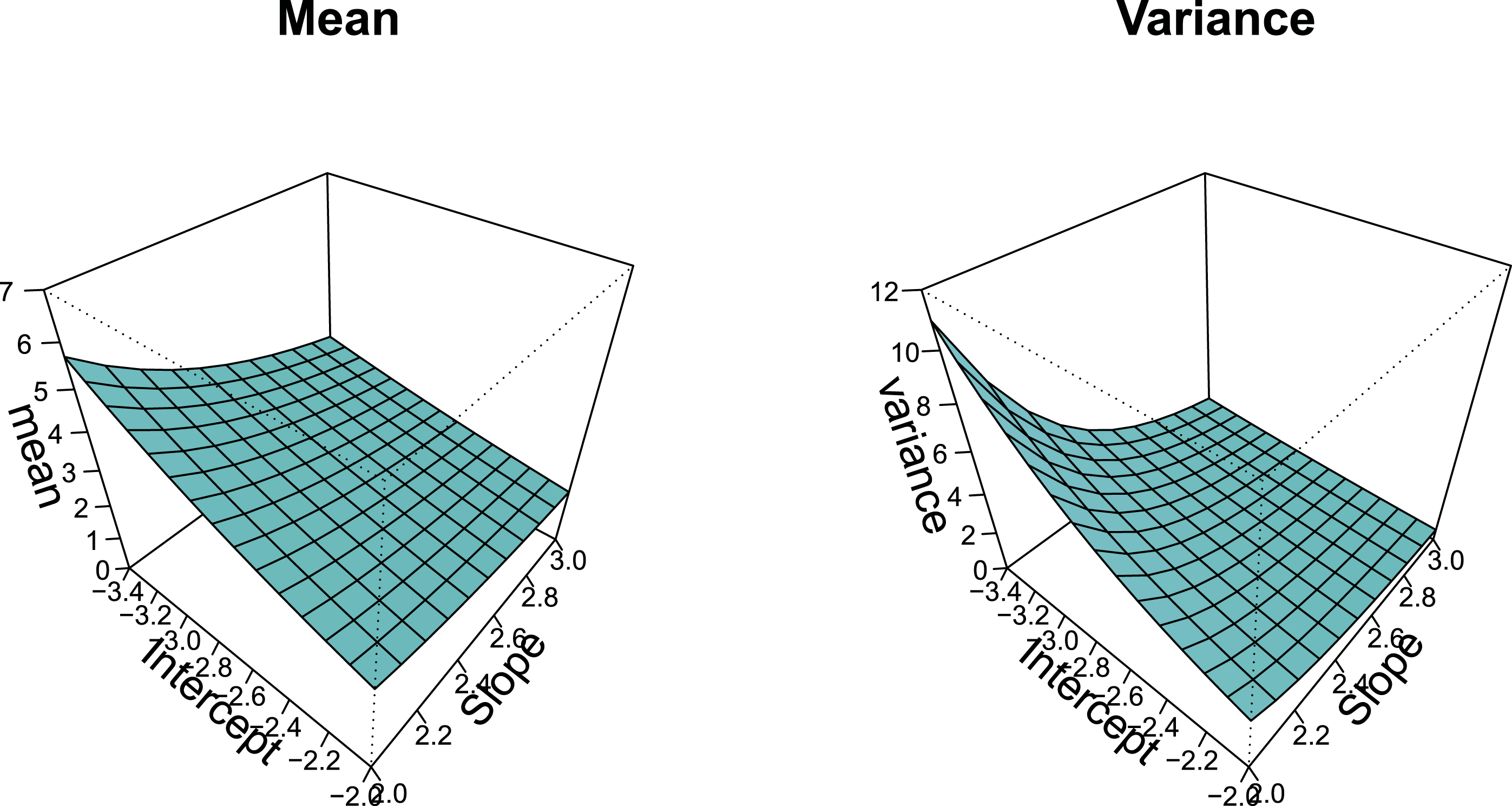

Estimation

If the general thresholds model holds the distribution function for observation Y_pi has the form

F_{p i} (y) = P (Y_{p i} \leq y) = 1 - F (θ_{p} - δ_{i} (y)) .

For observations Y_pi ∈ {0, 1, … } the probability mass function is given by

\begin{array}{l} f_{p i} (0) & = 1 - P (Y_{p i} > 0) = 1 - F (θ_{p} - δ_{i} (0)), \\ f_{p i} (r) & = P (Y_{p i} > r - 1) - P (Y_{p i} > r) = F (θ_{p} - δ_{i} (r - 1)) - F (θ_{p} - δ_{i} (r)), r = 1,2, \dots . \end{array}

Marginal likelihood estimation is obtained by assuming that person parameters are normally distributed, $θ_{p} \sim N (0, σ_{θ}^{2})$ . Maximization of the marginal log-likelihood can be obtained by integration techniques. We use numerical integration by Gauss-Hermite integration methods. Early versions for univariate random effects date back to Hinde (1982) and Anderson and Aitkin (1985) and are in common use to estimate item response models nowadays.

The marginal likelihood has the form

L (δ) = \prod_{p = 1}^{P} \int \prod_{i = 1}^{I} f_{p i} (y_{p i}) f_{0, σ_{θ}} (θ_{p}) d θ_{p},

where

f_{0, σ_{θ}} (θ_{p})

denotes the density of the person parameter

(N (0, σ_{θ}^{2}))

. This yields the log-likelihood

l (δ) = \log (L (δ)) = \sum_{p = 1}^{P} \log (\int \prod_{i = 1}^{I} f_{p i} (y_{p i}) f_{0, σ_{θ}} (θ_{p}) d θ_{p}) .

The corresponding score function s( δ ) = ∂l/∂ δ has components

\begin{array}{l} \frac{\partial l}{\partial δ_{i .}} & = \sum_{p = 1}^{P} \int \frac{\partial f_{p i} (y_{p i})}{\partial δ_{i .}} \prod_{l \neq i} f_{p i} (y_{p l}) f_{0, σ_{θ}} (θ_{p}) d θ_{p} / c_{p}, \\ \frac{\partial l}{\partial σ_{θ}} & = \sum_{p = 1}^{P} \int \prod_{i = 1}^{I} f_{p i} (y_{p i}) \frac{\partial f_{0, σ_{θ}} (θ_{p})}{\partial σ_{θ}} d θ_{p} / c_{p}, \end{array}

where

c_{p} = \int \prod_{i = 1}^{I} f_{p i} (y_{p i}) f_{0, σ_{θ}} (θ_{p}) d θ_{p}

. The derivatives of the density depend on the difficulty functions. For fixed difficulty function δ_i(y) = δ_i0 + δ_ig(y) one obtains

\begin{array}{l} \frac{\partial f_{p i} (y)}{\partial δ_{i 0}} = & - f (θ_{p} - δ_{i} (y - 1)) + f (θ_{p} - δ_{i} (y)), \\ \frac{\partial f_{p i} (y)}{\partial δ_{i}} = & - f (θ_{p} - δ_{i} (y - 1)) g (y - 1) + f (θ_{p} - δ_{i} (y)) g (y), \end{array}

where f(.) is the density corresponding to F(.), and δ_i(−1) = −∞.

Illustrative Simulation

We consider 10 items with logarithmic difficulty functions. The intercepts were δ_i0 = −6 + (i − 1)0.2 yielding the sequence −6, −5.8, −5.6, … , and slopes δ_i = 2 + (i − 1)0.1 yielding the sequence 2, 2.1, 2.2, …. The items are ordered, item 1 is the easiest item and item 10 the hardest, which is also seen from Figure 4, which shows the probabilities of a response larger than y for θ_p = 0 (only 9 items shown) and the corresponding response probabilities.

Figure 4.

Probabilities of a response larger than y for 10 items with true intercepts δ_i0 ∈ {−6, −5.8, −5.6, … } and slopes δ_i ∈ {2, 2.1, 2.2, … }.

Figure 5 shows the resulting parameter estimates and the true values (as dots) for P = 100 (200 repetitions), in the supplemental appendix results for P = 200 are given. It is seen that parameters are recovered very well. More important than accurate estimates of parameters is that the underlying distributions are estimated accurately. Since both parameters contribute to the difficulty even some underestimation of the slope can be compensated for by an overestimation of the intercept and vice versa. Therefore, the left picture in the third row shows the accuracy of estimates regarding the density of responses. It shows for all items the distance between the true (discrete) density and the estimated density for θ_p = 0

{Dist}_{i} = \sum_{r = 0}^{\infty} | P (Y_{p i} = r) - \hat{P} (Y_{p i} = r) |,

averaged across repetitions. It is seen that the distances between the true mass function and the estimated ones are very small, which is also seen from the two items for which the estimated person threshold functions of the first six simulated data sets are shown (second row). The right picture in the third row shows the correlation between the true person parameters and the corresponding estimates. It suggests that abilities are estimated rather well. The last row shows the standard errors of parameters (points) and the estimated standard errors over simulations as boxplots. The estimates are in the expected range although there is a weak tendency to underestimate the standard error.

Figure 5.

Simulation results for 10 items and P = 100 respondents; first row: intercepts and slopes, dots indicate true values; second row: person threshold functions for θ_p = 0 for items 1 and 8 and six estimated functions from the first six simulation runs; third row, first column: difference true and estimated densities for all items; third row, second column: correlation between true and estimated person parameters; forth row: standard errors, true and estimated, for item parameters.

Data-Driven Item Difficulty Functions

Fixed item difficulty functions are easy to handle but an appropriate function has to be chosen. If the form of the function is questionable it seems warranted to let the difficulty function be determined in a data-driven way from a wide range of possible functions. For illustration of the flexibility of the threshold model let us consider person p with cumulative probability mass function given by cpi(y_pi) = P(Y_pi > y_pi|θ_p, δ_i) = F(θ_p − δ_i(y)). Since parameters are only identifiable up to an additive constant, one can choose θ_p = 0 for this individual. Then for any function cpi(.) the item difficulty function can be computed by δ_i(y) = F⁻¹(cpi(y)). Thus, for any cumulative probability mass function one can find an item difficulty that fits this individual. Of course, if the item difficulty is determined for one individual, the model restricts the distribution of responses for all other individuals; however, it demonstrates that the choice of the item difficulty function can adapt quite flexibly to a wide range of possible distributions.

In the following, we consider a method to generate flexible difficulty functions. It can use fixed difficulty functions as a starting point or do without.

Modeling by Basis Functions

To obtain a wide range of item difficulties they can be approximated by a finite set of basis functions. We will consider two ways of using basis functions. One way is to let difficulty functions be determined solely by basis functions by assuming

δ_{i} (y) = \sum_{l = 0}^{M} δ_{i l} Φ_{i l} (y),

(3)

where Φ_il(.), l = 0, …, M are chosen basis functions. An attractive choice is B-splines as propagated and motivated extensively by Eilers and Marx (1996, 2021). They are very flexible and can closely approximate a variety of functions. Alternatively one can also use radial basis function, see, for example, Vidakovic (1999), Wood (2006a, 2006b), Ruppert et al. (2009), Wand (2000). The approach lets the data itself determine the form of the difficulty function and therefore the distribution of responses, it is not restricted to a fixed function as the logarithmic function.

The downside is that models are not nested. A model that uses basis functions is more flexible than a model with a logarithmic difficulty function, but it is not straightforward to compare the two models since the model that uses a fixed function is not a submodel of the basis functions model. A way to obtain nested models is to combine a fixed function with the basis function approach. Let the first two basis functions in (3) be given by

Φ_{i 0} (y) = 1, Φ_{i 1} (y) = \log (1 + y),

and the functions Φ_ij, j = 2, …, M be basis functions, for example, B-splines. Then the model that uses logarithmic difficulty functions is a submodel of the model with basis functions. The mixing of two types of basis functions yields nested models which can be compared by likelihood ratio tests.

For basis functions the log-likelihood functions are the same as in the case with fixed difficulty function. Only the derivatives have the more general form

\frac{\partial f_{p i} (y_{p i})}{\partial δ_{i j}} = - f (θ_{p} - δ_{i} (y_{p i} - 1)) Φ_{i j} (y_{p i} - 1) + f (θ_{p} - δ_{i} (y_{p i})) Φ_{i j} (y_{p i}),

where Φ_ij(−1) is defined by Φ_ij(−1) = 0.

The strategy we use here is to choose a moderate number of basis functions, say 8 to 10. It makes the difficulty functions sufficiently flexible without increasing the numbers of parameters too strongly. An alternative strategy is to use a larger number of basis functions, say 30 to 40, but then estimation becomes unstable, reliable estimates can be obtained only if one uses penalized maximum likelihood estimates, which restrict the variation of differences of parameters for adjacent basis functions, see Eilers and Marx (1996, 2021). Although the latter strategy is more flexible, it has the disadvantage that additional tuning parameters have to be selected. Moreover, likelihood ratio tests are not available since fitting is not based on maximum likelihood but on penalized maximum likelihood. For the choice of the number of basis functions in an application see also supplemental appendix.

Flexibility of Models

In the following, we briefly investigate the flexibility of the thresholds model. Several models can be used in count data item response theory, the simple Rasch count model, the negative binomial model, Conway–Maxwell models, or the thresholds model. Since typically it is not known which model generates the data it is useful if a model can adapt to quite different data generating mechanisms.

In a simulation study, we considered several data generating models and how differing models adapt to the generated data. As an example we give the results for 50 respondents and four items. The data generating models were

• (Poisson) the Poisson model with item parameters −2.4, −2.0, −1.6, −1.2 and σ_θ = 1,

• (CMGlobal) the Conway-Maxwell model with global dispersion with the same item parameters as the Poisson model, but the additional dispersion parameters ν₁ = ⋯ = ν₄ = 0.8,

• (CMDisp) the Conway-Maxwell model with varying dispersion with the same item parameters as the Poisson model, but the additional dispersion parameters (ν₁, ν₂, ν₂, ν₄) = (0.8, 0.9, 1.1, 1.2),

• (NegBin) the negative binomial model with the same expectation as the Poisson model but with strongly overdispersed items such that the variance is five times the mean of responses,

• (Thresholds) the thresholds model with logarithmic difficulty functions and item parameters (−6.02.0), (−5.62.2), (−5.22.4), (−4.82.6) for (δ_i0, δ_i), and σ_θ = 1.

Figure 6 shows the log-likelihoods and the AICs obtained when these models generate the data and are also used to fit the data (100 repetitions). In addition, the thresholds model with splines was fitted (ThreshSpl). It is seen that the splines model always yields the best fit in terms of maximum log-likelihood. It shows that the model is able to fit data that were generated by any of the models that were used. The thresholds model with fixed difficulty functions fits well if it is the data generating model but is not flexible enough if the Poisson or the Conway–Maxwell model generate the data. However, it fits comparatively well if the generating model is the negative binomial model with overdispersion. It is interesting how models fit if one takes the number of fitted parameters into account by considering the AIC. Then, the splines model shows good performance for most models, in particular the fit in terms of AIC is comparable to the fits of Conway–Maxwell models if the latter are the data generating models. In the case of the negative binomial model the performance is stronger in terms of AIC. If the threshold model generates the data the threshold model with fixed difficulty functions performs best as was to be expected. Conway–Maxwell models perform worse and do not adapt very well to the probability structure of thresholds models, which is somewhat hidden by the inclusion of the Poisson fit, which in this case shows very poor performance.

Figure 6.

Simulation results for differing data generating models (P=50); first row: Poisson model, second row: Conway-Maxwell (CM) with global dispersion, third row: CM with varying dispersion, fourth row: negative binomial model; fifth row: thresholds model; left column: log-likelihood, right column: AIC.

Application

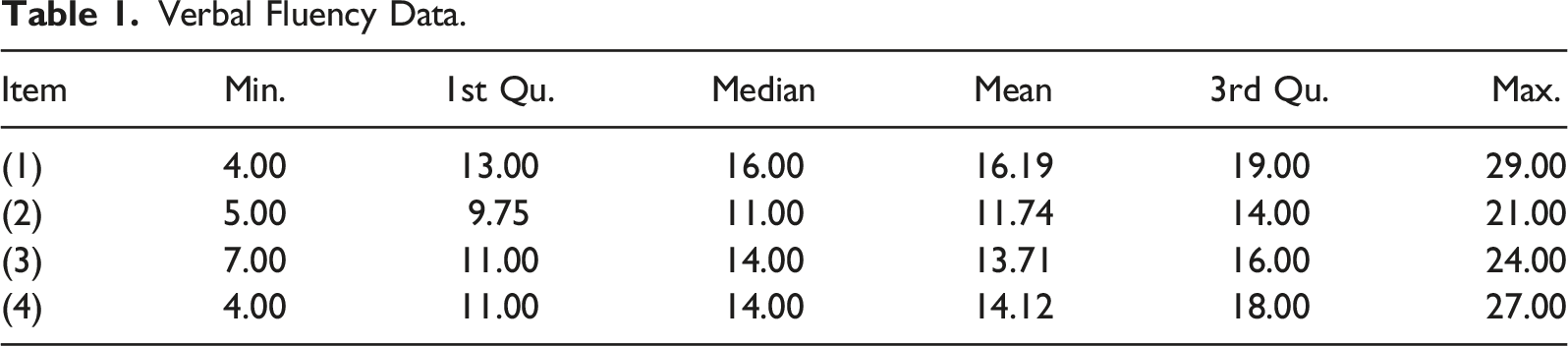
Forthmann et al. (2020) used a data set with four commonly used verbal fluency tasks, which are available at https://osf.io/38zsm/. The data set includes two semantic fluency tasks, namely, animal naming (item 1) and naming things that can be found in a supermarket (item 4) and two letter fluency tasks, words beginning with letter f (item 2) or letter s (item 3). The participants had 1 minute to complete each of the verbal fluency tasks. In our analysis, we use the 192 individuals that responded to all items.

Table 1 shows some descriptive measures for the marginal distribution of item responses. The largest means are found for item 1 and item 4, which suggests that the items are easier than items 2 and 3. A more careful analysis is obtained by using the count threshold model with differing degrees of freedom. We consider first models with logarithmic difficulty functions. Model 1 assumes that difficulties have common slopes, model 2 is more general and allows for varying slopes. Figure 7 shows the estimated difficulty functions, person threshold functions for value θ = 0 and densities. The left column shows the fits of model 1 with common slopes, the right column shows the results for varying slopes (model 2). The rather restrictive model with common slopes suggests that items 3 and 4 have the same difficulty and yield identical conditional distributions. The more flexible model shows differing conditional distributions especially for these two items. Although the peak is the same for both items, item 4 shows a much larger dispersion than item 3. The dispersion seems to vary strongly across items. It turns out that the more general model shows a significantly better fit and the hypotheses of common slopes should be rejected. The corresponding log-likelihood test is 54.66 on 3 df (log-likelihoods for the models are given in Table 2).

Table 1.

Verbal Fluency Data.

Item	Min.	1st Qu.	Median	Mean	3rd Qu.	Max.
(1)	4.00	13.00	16.00	16.19	19.00	29.00
(2)	5.00	9.75	11.00	11.74	14.00	21.00
(3)	7.00	11.00	14.00	13.71	16.00	24.00
(4)	4.00	11.00	14.00	14.12	18.00	27.00

Figure 7.

Difficulty functions, person threshold functions, P(Y > y), for value θ = 0 and densities for verbal fluency data; left: common slope, right: varying slopes.

Table 2.

Log-Likelihoods, AIC, Number of Parameters, and Mixture Standard Deviations.

		Log-likelihood	Param	AIC	${\hat{σ}}_{θ}$
(1)	Logarithmic diff function, common slopes	−2065.39	6	4142.79	1.041
(2)	Logarithmic diff function, varying slopes	−2038.06	9	4094.11	1.041
(3)	Eight splines	−1994.75	33	4055.50	0.972
(4)	Logarithmic diff function + eight splines	−1990.40	41	4062.80	0.973
(P)	Poisson model	−2072.4	5	4154.8	0.194
(CMG)	Conway–Maxwell model, global dispersion	−2032.3	6	4076.6	0.217
(CMV)	Conway–Maxwell model, varying dispersion	−2011.1	9	4040.1	0.211

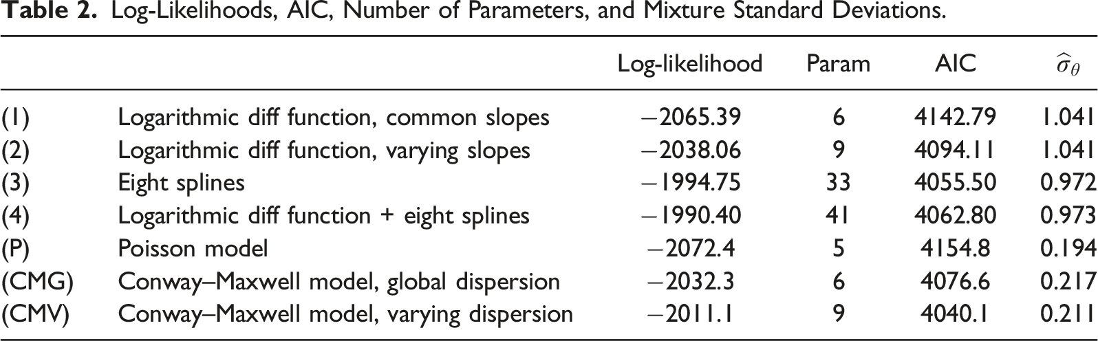
Figure 8 shows the posterior estimates of person abilities plotted against the total score $Y_{p \cdot} = Σ_{i} Y_{p i}$ . As was to be expected, there is a strong link between the sum score and the ability of persons, although the correlation is high the link is rather monotone than linear.

Figure 8.

Posterior estimates of person parameters against sum score of persons.

We also considered the more general model with data-driven choice of difficulty functions. Model 3 uses basis functions only to approximate the difficulty functions while model 4 uses a combination of the logarithmic function and basis functions. In both models the number of cubic B-splines was 8, which provides enough flexibility but does not inflate the number of parameters. Cubic splines are a natural and widely used choice since they yield rather smooth curves, splines of higher order typically yield no discernible change in fitted curves. Thus, each item has 8 parameters in model 3 (only B-splines) and 10 parameters in model 4 (8 B-splines parameters, intercept and slope on logarithmic function). The difference between the two models is negligible as is seen from Figure 9. Also the likelihood ratio test that compares the two models shows that there is no significant difference (8.70 on 8 df). Model 4 has the advantage that it can be directly compared to model 2 since model 2 is a submodel of model 4. The likelihood ratio test yields 95.12 on 32 df, which means the difference is highly significant, and the model that allows for more flexible difficulty functions is more appropriate.

Figure 9.

Difficulty functions, person threshold functions, P(Y > y), for value θ = 0 and densities for verbal fluency data; left: logarithmic plus B-splines, right: B-splines.

We also fitted the Poisson model and extensions by using the R package glmmTMB, for a detailed description of the models and how to fit them see Forthmann et al. (2020). Table 2 shows the results for three models, the Poisson Rasch model (M), the Conway–Maxwell model with global dispersion (CMG), and the Conway–Maxwell model with varying dispersion (CMV). It is seen that in terms of AIC the Poisson model and the Conway–Maxwell model with global dispersion fit the data less well than the thresholds models (3) and (4), the best fit was found for the Conway–Maxwell model with varying dispersion. The largest log-likelihood value was found for model (4) but since it has more parameters than model (3) and the Conway–Maxwell model the AIC is larger. It is worth mentioning that posterior estimates are highly correlated for the models. For example, the person parameters of the threshold model with varying slopes (shown in Figure 8) have correlation 0.9906 with the person parameters of the Poisson model, 0.9924 with the global dispersion Conway–Maxwell model, and 0.9901 with the varying dispersion Conway–Maxwell model. For the latter model, the computational effort is rather high as compared to threshold models.

Concluding Remarks

Item response count models as alternatives to fixed distribution models have been introduced. The models allow for very flexible modeling of responses that can account for a wide range of response distributions that may vary across items. It has been demonstrated that the model also fits well if data are generated by the Conway–Maxwell distribution. The item characteristics of the model are summarized in difficulty functions, which are easily accessible in the form of plots. In the simplest case, difficulty functions are ordered, indicating that items are ordered in a simple way. In the considered application more flexible modeling with crossing item difficulties turned out to be more appropriate.

It has also been demonstrated that the model yields good parameter recovery. In the simulation and application sections we used the package glmmTMB to fit the Conway–Maxwell model, see Forthmann et al. (2020). For the fitting of the threshold model an R program has been written that uses the function gauss.hermite from the package spatstat, and the package splines when fitting difficulty functions that are expanded in B-splines. Software that can be used to fit models and compute the results shown in previous sections will be made available on GitHub.

Supplemental Material

Supplemental Material - Flexible Item Response Models for Count Data: The Count Thresholds Model

Supplemental Material for Flexible Item Response Models for Count Data: The Count Thresholds Model by Gerhard Tutz in Applied Psychological Measurement

Footnotes

Acknowledgments

I want to thank Boris Forthman for providing the data set and the code to fit Conway-Maxwell type models.

Declaration of Conflicting Interests

The author(s) declared no potential conflicts of interest with respect to the research, authorship, and/or publication of this article.

Funding

The author(s) received no financial support for the research, authorship, and/or publication of this article.

ORCID iD

Gerhard Tutz

Supplemental Material

Supplemental Material for this article is available online.

References

Anderson

D. A.

Aitkin

(1985). Variance component models with binary response: Interviewer variability. Journal of the Royal Statistical Society Series B, 47(2), 203–210. https://doi.org/10.1111/j.2517-6161.1985.tb01346.x

Doebler

Holling

(2016). A processing speed test based on rule-based item generation: An analysis with the rasch Poisson counts model. Learning and Individual Differences, 52, 121–128. https://doi.org/10.1016/j.lindif.2015.01.013

Eilers

P. H.

Marx

B. D.

(2021). Practical smoothing: The joys of P-splines. Cambridge University Press.

Eilers

P. H. C.

Marx

B. D.

(1996). Flexible smoothing with B-splines and penalties. Statistical Science, 11(2), 89–121. https://doi.org/10.1214/ss/1038425655

Forthmann

Doebler

(2021). Reliability of researcher capacity estimates and count data dispersion: A comparison of Poisson, negative binomial, and Conway-Maxwell-Poisson models. Scientometrics, 126(4), 3337–3354. https://doi.org/10.1007/s11192-021-03864-8

Forthmann

Gühne

Doebler

(2020). Revisiting dispersion in count data item response theory models: The Conway–Maxwell–Poisson counts model. British Journal of Mathematical and Statistical Psychology, 73(1), 32–50. https://doi.org/10.1111/bmsp.12184

Forthmann

Holling

Çelik

Storme

Lubart

(2017). Typing speed as a confounding variable and the measurement of quality in divergent thinking. Creativity Research Journal, 29(3), 257–269. https://doi.org/10.1080/10400419.2017.1360059

Hinde

(1982). Compound Poisson regression models. In Gilchrist

(Ed.), GLIM 1982 International conference on generalized linear models (pp. 109–121). Springer-Verlag.

Huang

(2017). Mean-parametrized Conway–Maxwell–Poisson regression models for dispersed counts. Statistical Modelling, 17(6), 359–380. https://doi.org/10.1177/1471082x17697749

10.

Hung

L.-F.

(2012). A negative binomial regression model for accuracy tests. Applied Psychological Measurement, 36(2), 88–103. https://doi.org/10.1177/0146621611429548

11.

Jansen

M. G.

(1995). The Rasch Poisson counts model for incomplete data: An application of the EM algorithm. Applied Psychological Measurement, 19(3), 291–302. https://doi.org/10.1177/014662169501900307

12.

Jansen

M. G.

van Duijn

M. A.

(1992). Extensions of Rasch’s multiplicative Poisson model. Psychometrika, 57(3), 405–414. https://doi.org/10.1007/bf02295428

13.

Jansen

P. G.

Roskam

E. E.

(1986). Latent trait models and dichotomization of graded responses. Psychometrika, 51(1), 69–91. https://doi.org/10.1007/bf02294001

14.

Lord

F. M.

Novick

M. R.

(2008). Statistical theories of mental test scores. Information Age Publishing Inc.

15.

McCullagh

Nelder

J. A.

(1989). Generalized linear models (2nd ed.). Chapman & Hall.

16.

Rasch

(1960). Probabilistic models for some intelligence and attainment tests. Danish Institute for Educational Research.

17.

Rasch

(1961). On general laws and the meaning of measurement in psychology. In Proceedings of the fourth Berkeley symposium on mathematical statistics and probability (4, pp. 321–333). Statistical Laboratory of the University of California.

18.

Roskam

E. E.

Jansen

P. G.

(1989). Conditions for Rasch-dichotomizability of the unidimensional polytomous rasch model. Psychometrika, 54(2), 317–332. https://doi.org/10.1007/bf02294523

19.

Ruppert

Wand

M. P.

Carroll

R. J.

(2009). Semiparametric regression during 2003 – 2007. Electronic Journal of Statistics, 3, 1193–1256. https://doi.org/10.1214/09-ejs525

20.

Samejima

(1973). Homogeneous case of the continuous response model. Psychometrika, 38(2), 203–219. https://doi.org/10.1007/bf02291114

21.

Samejima

(2016). Graded response model. In van der Linden

(Ed), Handbook of item response theory (pp. 95–108).

22.

Shmueli

Minka

T. P.

Kadane

J. B.

Borle

Boatwright

(2005). A useful distribution for fitting discrete data: Revival of the conway–maxwell–Poisson distribution. Journal of the Royal Statistical Society: Series C (Applied Statistics), 54(1), 127–142. https://doi.org/10.1111/j.1467-9876.2005.00474.x

23.

Silvia

P. J.

Beaty

R. E.

Nusbaum

E. C.

(2013). Verbal fluency and creativity: General and specific contributions of broad retrieval ability (gr) factors to divergent thinking. Intelligence, 41(5), 328–340. https://doi.org/10.1016/j.intell.2013.05.004

24.

Süß

H.-M.

Oberauer

Wittmann

W. W.

Wilhelm

Schulze

(2002). Working-memory capacity explains reasoning ability and a little bit more. Intelligence, 30(3), 261–288. https://doi.org/10.1016/s0160-2896(01)00100-3

25.

Tutz

(2021). Flexible predictive distributions from varying-thresholds modelling. Technical report. https://arxiv.org/abs/2103.13324

26.

Tutz

(2022). Item response thresholds models: A general class of models for varying types of items. Psychometrika. https://doi.org/10.1007/s11336-022-09865-7

27.

Vidakovic (1999). Statistical modelling by wavelets. Wiley Series in Probability and StatisticsWiley.

28.

Wand

M. P.

(2000). A comparison of regression spline smoothing procedures. Computational Statistics, 15(4), 443–462. https://doi.org/10.1007/s001800000047

29.

Wood

S. N.

(2006a). On confidence intervals for generalized additive models based on penalized regression splines. Australian & New Zealand Journal of Statistics, 48(4), 445–464. https://doi.org/10.1111/j.1467-842x.2006.00450.x

30.

Wood

S. N.

(2006b). Thin plate regression splines. Journal of the Royal Statistical Society, Series B, 65(1), 95–114. https://doi.org/10.1111/1467-9868.00374

Supplementary Material

Please find the following supplemental material available below.

For Open Access articles published under a Creative Commons License, all supplemental material carries the same license as the article it is associated with.

For non-Open Access articles published, all supplemental material carries a non-exclusive license, and permission requests for re-use of supplemental material or any part of supplemental material shall be sent directly to the copyright owner as specified in the copyright notice associated with the article.

0.00 MB

0.27 MB