



Abstract
Our study examines whether aggressive revenue management by a supplier is greater when the supplier and their major customer engage the same office-level auditor and when significant purchases are made by the major customer from the supplier. We posit that the auditor is more accommodating to clients who are jointly audited by the same office-level auditor because of the implicit threat of losing not just the supplier client but also the major customer client. The threat arises from the potential loss of synergies of a jointly planned audit engagement when significant purchases are made by the major customer. We find that income-increasing discretionary revenue is positively associated with the major customer’s percentage of purchases from the supplier when the same office-level auditor is engaged by the supplier and their major customer. We fail to find a statistically significant association when they engage a different office-level auditor or a different audit firm. Our findings provide evidence that office-level auditors tolerate greater aggressive revenue management when they have clients who are partners in the same supply chain and when greater audit synergies are at stake. In addition, our results are partly explained by supplier clients who have interlocking directors with major customers and significant influence.
Keywords
Introduction
This article investigates whether a client (the supplier) aggressively manages revenue when they engage the same office-level auditor as their major customer (hereafter, a supply chain auditor), 1 and when the major customer purchases a large percentage from the supplier (hereafter, economic dependence). A major customer is an important party to a supply chain because it comprises a substantial percentage (at least 10%) of the supplier’s revenue (Financial Accounting Standards Board [FASB], 2017a, ASC 280-10-50-42). We predict that a supply chain auditor is more accommodating to the supplier client’s aggressive revenue management attempts because of the implicit threat of losing both the supplier and major customer client (hereafter, the supply chain clients). The threat stems from audit synergies of the audits of the supply chain clients and the clients’ need to protect shared proprietary information. We also predict that interlocking directors, and significant influence between the supply chain clients, play a major role in our setting. Our study extends a growing stream of research about supply chain management in the accounting and auditing literature (e.g., Bowen, DuCharme, & Shores, 1995; Chen, Chang, Chen, & Kim, 2014; Hui, Klasa, & Yeung, 2012; Raman & Shahrur, 2008).
Our study is interesting because revenue management is one of the most pervasive forms of earnings manipulation (Dechow & Schrand, 2004). Prior studies have examined whether earnings management exists within a supply chain (Bowen et al., 1995; Hui et al., 2012; Raman & Shahrur, 2008); however, these same studies have not examined whether revenue management exists within a supply chain, and whether it varies by the engagement of a supply chain auditor. While Chen et al. (2014) find that audit fees are lower for supplier clients who engage a supply chain auditor, it is not clear whether lower audit fees adversely affect audit quality. We examine a particular setting where audit synergies create incentives for the auditor to tolerate attempts by the supplier client to inflate reported revenue through early recognition (hereafter, aggressive revenue management).
Arguably, a supplier and an economically dependent major customer, who engage a supply chain auditor, are viewed by the auditor as a larger client. The supply chain auditor could acquiesce to reduce the implicit threat of losing not just one client (the supplier client) but two (the supply chain clients). As well, when the supplier and major customer share common directors (hereafter, interlocking directors) or they have significant influence between themselves, there are greater audit synergies and shared proprietary information but weaker corporate governance. If the implicit threat of losing both clients is sufficient, aggressive revenue management by the supplier client should be higher in this setting.
A case in point is The Coca-Cola Company (Coke) who engaged a supply chain auditor for the 1999 fiscal year end. In 2000, a shareholder lawsuit, led by the Carpenters Health & Welfare Fund of Philadelphia & Vicinity, complained that Coke failed to disclose material facts including “channel stuffing” to some of its bottlers in 1999; the case was settled with Coke admitting no wrongdoing (“Coca-Cola agrees to $137.5 mln,” 2008). As well, allegations of channel stuffing were made, among others, in another case involving sales to a major customer, Coca-Cola Enterprises, Inc. (CCE) in the 1990s to 2004 (International Brotherhood of Teamsters v. Coca-Cola Co., 2007). Thus, it appears that there is potential for aggressive revenue management in this setting.
We use aggressive revenue management to measure audit quality for two reasons: First, revenue is not only one of the most important performance measures for assessing future prospects (FASB, 2017b), but it is also one of the most pervasive forms of earnings management (Dechow & Schrand, 2004). Current revenue accounting standards are “complex, detailed and disparate” (FASB, 2017b), and allow greater discretion, particularly when transactions are more complex and unusual (American Institute of Certified Public Accountants [AICPA], 1999). Prior studies suggest several incentives to inflate revenue (Edmonds, Leece, & Maher, 2013; Ertimur, Livnat, & Martikainen, 2003; Marquardt & Wiedman, 2004; Plummer & Mest, 2001; Rees & Sivaramakrishnan, 2007), but very few (Krishnan & Yu, 2012) have measured audit quality with aggressive revenue management. 2 Second, our inferences are more internally valid because discretionary revenue models (Stubben, 2010) are more precise and less biased than conventional discretionary accrual models. Namely, discretionary revenue models focus only on one component of earnings (revenue), and they better detect firms that are targeted by U.S. Securities Exchange Commission (SEC) enforcement actions. We measure aggressive revenue management as positive-signed (i.e., income-increasing) values from Stubben’s (2010) model.
To examine whether aggressive revenue management varies in our setting, we examine whether positive-signed discretionary revenue of the supplier is associated with engaging a supply chain auditor when the major customer is more economically dependent. Economic dependence captures the relative importance of the major customer in the supply chain audit by the relative importance of its purchases from the supplier (Hui et al., 2012; Porter, 1980), which we measure as the percentage of the major customer’s total cost of goods sold (PFS%). To control for potential endogeneity, arising from aggressive revenue management firms self-selecting, we employ a Heckman (1979) model. In our robustness tests, we control for the choice of a supply chain auditor.
From our sample (2003-2012), we find that positive-signed discretionary revenue is positively associated with PFS% when a supply chain auditor is engaged. In fact, we fail to find a statistically significant association when a nonsupply chain auditor is engaged—one that is the same audit firm engaged by the major customer, but from a different audit office, or an entirely different audit firm. In addition, our results are partly explained by supply chain clients who have interlocking directors and significant influence. Our results are economically significant—Mean marginal positive-signed discretionary revenue for supplier clients is 0.50% of sales revenue, and even greater when there are interlocking directors (1.09%) and significant influence present (2.21%).
Our results are robust to several tests. We measure aggressive revenue management with the likelihood of meeting or beating analyst revenue forecasts (with sufficient discretionary revenue), revenue-related restatements, and three other discretionary revenue models. We find support for our argument that supply chain auditors are threatened by losing not just one client but two, by the fact that an economically dependent major customer is more likely to change auditors in the current period when the supplier changed in the prior period and when the supplier has positive-signed discretionary revenue. As well, we find evidence of economic bonding between the supply chain auditor and the supplier client, by the fact that a supply chain auditor is less likely to switch than a nonsupply chain auditor, when aggressive revenue is greater in the prior period. Finally, we find that our main result is less likely when the supply chain auditor is a joint national-office-level industry specialist, which corroborates prior studies that find clients of industry specialist auditors are associated with higher audit quality (e.g., Reichelt & Wang, 2010).
Our article contributes as follows. First, we extend Chen et al. (2014) who show that supply chain auditors charge lower audit fees. We show that when a supplier and an economically dependent major customer engage a supply chain auditor, aggressive revenue management by the supplier is less constrained. Second, our article extends prior studies examining interlocking directors and their association with earnings management and auditor choice (Chiu, Teoh, & Tian, 2013; Davison, Stening, & Wai, 1984). We show a setting where a supplier’s aggressive revenue management is positively and jointly associated with a supply chain auditor, interlocking directors, and an economically dependent major customer. Third, we extend prior studies that examine the variation in office-level audit quality (e.g., Reynolds & Francis, 2000). We show a setting where a supplier client and an economically dependent major customer are apparently viewed as one larger client by the supply chain auditor’s office, and supplier revenue quality is lower.
The rest of the article is organized as follows: The “Literature Review and Empirical Predictions” section reviews the related literature and develops empirical predictions. The “Data and Sample” section describes the data and sample. The “Analysis of Positive-Signed Discretionary Revenue” section presents estimation models and the main results. The “Robustness Tests” section presents supporting robustness tests. The “Conclusion” section concludes.
Literature Review and Empirical Predictions
Background to Major Customers and Aggressive Revenue Management
Major customers are an important party to a supply chain. By definition, major customers comprise at least 10% of their supplier’s total revenue (FASB, 2017a, ASC 280-10-50-42). The accounting standard requires that firms disclose the fact that they have major customers and the dollar amount of sales to each. U.S. Securities and Exchange Commission (2017), under Regulation S-K (17 CFR 229.101[c][1][vii]), further requires that firms identify the major customer’s name. Understandably, these requirements recognize that having only a few major customers imposes significant business risk (McEwen, 1990).
Within the supply chain, the presence of major customers provides incentives for suppliers to manage earnings. Prior literature finds that suppliers choose accounting methods and accruals to improve customer perceptions (Bowen et al., 1995; Raman & Shahrur, 2008). Bowen et al. (1995) find that supplier firms are more likely to choose income-increasing accounting methods when they have ongoing implicit claims from customers. Raman and Shahrur (2008) find that firms larger than their customers (e.g., Coke vs. CCE) have a higher magnitude of discretionary accruals when there is a greater level of relationship-specific investments (investments specific to a customer).
While these studies provide evidence that suppliers manage earnings, we investigate a more pervasive form—revenue management. Revenue management is the most frequent source of SEC Accounting and Auditing Enforcement Releases (AAERs; Dechow & Schrand, 2004). 3 In this study, we refer to aggressive revenue management when managers inflate revenue accrual estimates, predicated by economic incentives such as revenue targets. Distributional tests suggest that earnings are managed upward by managing revenues upward to improve analyst ratings (Plummer & Mest, 2001). Stock market premiums from analyst earnings benchmark beating are accentuated by revenue benchmark beating (Rees & Sivaramakrishnan, 2007). Managers are penalized with smaller bonuses when they miss analyst revenue benchmarks, incremental to the penalty for missing analyst earnings benchmarks (Edmonds et al., 2013). Investors value analyst revenue surprises more than expense surprises, particularly among growth firms (Ertimur et al., 2003). Revenue benchmark beating increases with investor valuation of revenue surprises, particularly among relatively young firms (Zhao, 2017).
Arguably, aggressive revenue management is achieved by estimating revenue accruals in the most optimistic manner. To provide context, we provide the following examples of revenue accrual estimates from our sample of clients who engaged a supply chain auditor (source: Form 10-K filings). Ultratech, Inc. (2007), is a developer and manufacturer of photolithography and laser thermal equipment for use by manufacturers such as their major customer, Intel. Their revenue includes multiple element arrangements that require estimates of the fair value of undelivered individual software, hardware, and service agreement elements (fiscal year 2006 10-K filing). Seagate Technology (2004) designs and manufactures rigid drives for use by manufacturers and distributors, including their major customer, Hewlett–Packard. Their revenue includes estimates of sales incentive allowances and sales returns (fiscal year 2004 10-K filing).
Supply Chain Auditor Benefits and Costs to the Supplier and Major Customer
We posit that engaging a supply chain auditor incentivizes the supplier client to aggressively manage revenues; thus, we begin by examining the supply chain clients’ incentives to engage a supply chain auditor. We define a supply chain auditor as one who audits both the supplier client and the major customer of the supplier from the same audit office. Figure 1 illustrates three examples of which the first is a supply chain auditor. The second and third examples are not supply chain auditors because the major customer engages either a different audit office of the same audit firm or an entirely different audit firm.
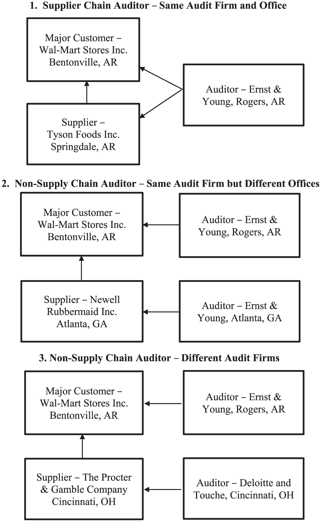
Supplier, major customer, and auditor examples.
The choice of a supply chain auditor is partly determined by minimizing costs which stem from the physical proximity of the audit office to the supply chain clients, audit synergies from jointly planned and executed audits, and the integrity of shared proprietary information between supply chain clients. First, clients more often engage an auditor from the same metropolitan area as their headquarters (Francis, Reichelt, & Wang, 2005) to minimize audit costs, including auditor’s costs of travel, communication, coordination, and acquisition of soft information (Jensen, Kim, & Yi, 2015). When supply chain clients are in the same metropolitan area (see Figure 1), engaging a supply chain auditor minimizes these costs. Next, audit synergies result in cost savings from knowledge spillovers, and when the supply chain auditor can feasibly and jointly plan and execute the audits of the supply chain clients (Chen et al., 2014). Audit synergies are feasible when intercompany transactions between the supply chain clients are sufficiently large in volume and magnitude. Arguably, audit synergies increase with the major customer’s proportion of purchases from the supplier. Finally, the integrity of proprietary information, shared between the supply chain clients (e.g., relationship-specific assets), is better maintained by engaging a supply chain auditor. Similarly, competing client firms typically engage different audit firms (e.g., Aobdia, 2015).
A case in point is Coke and CCE, who engaged the same audit firm (Ernst & Young) from the Atlanta office, where both clients are headquartered. Coke supplies CCE with concentrate and syrup which CCE uses to produce bottled and canned soft drinks for sale to retailers and other distributors. In 1999, CCE is a major customer of Coke accounting for 17% of Coke’s sales revenue (Coke’s 2000 10-K filing). CCE’s purchases from Coke accounted for 45% of its cost of goods sold (CCE’s, 2000 10-K filing). Coke is a sole supplier of unique brands to CCE. Engaging the same office-level auditor minimizes audit costs (including audit fees) for both parties while better maintaining the integrity of Coke’s proprietary information (e.g., marketing plans and soft drink recipes).
However, this setting has the potential to increase economic bonding between the supply chain auditor and the supply chain clients. In turn, there is potentially greater tolerance for aggressive revenue management attempts by the supplier client and potentially higher related costs. 4
Revenue Management Benefits and Costs to the Supply Chain Auditor
Whether a supply chain auditor will indeed acquiesce to the supplier client’s revenue management attempts will depend on whether the supply chain auditor’s benefits exceed their costs. As shown in Figure 1, a supply chain auditor differs by the location of their office, which makes the office an important level of analysis for several reasons. The office level involves key decisions such as the appropriate audit report (Reichelt & Wang, 2010) and partner compensation (e.g., Trompeter, 1994). The office retains deep personal knowledge of the client by key audit staff which cannot easily be distributed to other offices within the firm (Francis et al., 2005), including knowledge of the client’s revenue management practices. Thus, lower quality audits tend to cluster in certain offices (Francis & Michas, 2013), suggesting that auditors indeed acquiesce at the office level, such as by expending less effort to detect revenue management and by waiving audit adjustments.
An important consideration in our study is that audit synergies make the supply chain audit engagement more efficient (Chen et al., 2014). Audit synergies stem from the supply chain auditor having knowledge of both supply chain clients, which can be used to design more efficient audit procedures and with less duplication of effort. 5 Thus, both clients incur lower audit costs. Examples of efficiencies include knowledge of the supply chain industry and associated risks, knowledge of the accounting systems that have mirror effects (e.g., the revenue/receivables/receipts system of the supplier and the purchases/payables/payments system of the major customer), confirmation of in-transit inventory for the purpose of cutoff tests, accounting for leases and sale of operating assets between the two parties, and accounting for equity investments. 6
Considering that the supply chain audit is more efficient, two incentives pressure the supply chain auditor to be more tolerant of the supplier’s aggressive revenue management attempts. First, there is the threat of losing the supplier client and related audit synergies. If the supply chain auditor does not acquiesce to the supplier client, the client can depart, and the auditor will not only lose the profits from the supplier client but also the audit synergies from the jointly planned audit.
Second, if the loss of the supplier’s audit synergies is sufficiently high, there is the threat that the major customer client will switch auditors. Specifically, the loss of the supplier client to the auditor leads to the loss of audit synergies, making the audit more costly for the major customer. If switching costs are sufficiently low, the major customer will engage another supply chain auditor, particularly when the major customer’s purchases from the supplier are a larger percentage of their total (i.e., greater audit synergies and shared proprietary information).
Auditors, however, have incentives to constrain the supplier client’s aggressive revenue management attempts. Two major incentives are higher litigation costs arising from auditor’s “deep pockets,” and investor’s recovery of damages for auditor misconduct (e.g., Casterella, Jensen, & Knechel, 2010) and higher regulatory costs (e.g., Boone, Khurana, & Raman, 2015). However, a counterargument is that the auditor may not view the supply chain audit as a significant risk because courts and regulators will not view the two supply chain clients as one large client but rather as two separate legal entities. In fact, the major customer has minimal legal exposure because they may be unaware of the supplier’s aggressive revenue management. In short, whether the auditor’s benefits exceed their costs is an empirical question.
Assuming that the supply chain auditor’s benefits exceed their costs, we predict that when an economically dependent major customer and their supplier engage a supply chain auditor, the greater percentage of purchases by the major customer from the supplier benefits the two supply chain clients with lower costs (audit synergies and integrity of shared proprietary information). However, audit synergies impose an economic bond between the supply chain auditor and the supply chain clients; thus, there is less auditor constraint of the supplier client’s aggressive revenue management attempts. This scenario is more likely when revenue is a performance benchmark of the supplier.
To evaluate this prediction, we proxy aggressive revenue management with positive-signed discretionary revenue (Stubben, 2010), which reflects successful attempts by management to aggressively manage revenue. Like abnormal accrual measures, it is a financial reporting quality measure that detects “within GAAP” (generally accepted accounting principles) earnings manipulation. While it is less likely to give rise to a material misstatement, it arguably captures the likelihood of more extreme misstatements (DeFond & Zhang, 2014). Our main empirical prediction is as follows:
Interlocking Directors and Revenue Management
We refer to an interlocking director as one who serves on the board of the two supply chain clients. Interlocking directors are a valuable resource to supply chain clients by possessing common information and expertise (Mizruchi, 1996), including proprietary information. Interlocking directors have even been found to be associated with the appointment of the same audit firm (Davison et al., 1984), suggesting that they are a resource to the audit.
While interlocking directors are a valuable resource, they are arguably a weaker form of corporate governance. The financial economics and accounting literature shows that interlocking directors are associated with backdating of stock options (Bizjak, Lemmon, & Whitby, 2009) and earnings management contagion (Chiu et al., 2013). Consequently, we expect that weaker corporate governance demands lower audit quality, and specify our second prediction as follows:
Equity Investments and Revenue Management
Following the previous discussion, supply chain parties form networks not only through interlocking directors but also through significant influence from equity investments. Equity investments can take the form of investments by the supplier in the major customer and by the major customer in the supplier. Under FASB’s codification (ASC 323-10-15), significant influence is achieved when the investor can significantly influence operating and financing policies of the investee, and when the investor owns between 20% and 50% of the voting shares of the investee. The accounting standard provides guidance by listing several conditions, which includes the presence of material intra-entity transactions. 7
The implication is that transactions between the supply chain clients are larger, and the major customer is more economically dependent on the supplier. 8 The larger economic dependence leads to greater audit synergies and economic bonding. As well, the equity investments involve a greater likelihood of relation-specific investments that possess shared proprietary information between the two parties.
Significant influence, however, arguably reduces the effectiveness of corporate governance, financial reporting quality, and the demand for audit quality because intra-entity transactions are also related party transactions (ASC 850-10-20). The FASB (1982) has expressed concern that related party transactions affect the reliability of financial statements, which increases the risk of financial statement manipulation, and internal auditors rate them as the second most effective red flag to identifying opportunities to commit fraud (Moyes, Lin, & Landry, 2005).
In short, significant influence increases audit synergies and the likelihood of shared proprietary information, thus increasing the threat to the supply chain auditor of losing both supply chain clients. As well, greater related party transactions incur a weaker form of corporate governance; thus, aggressive revenue management is more likely to be tolerated.
Data and Sample
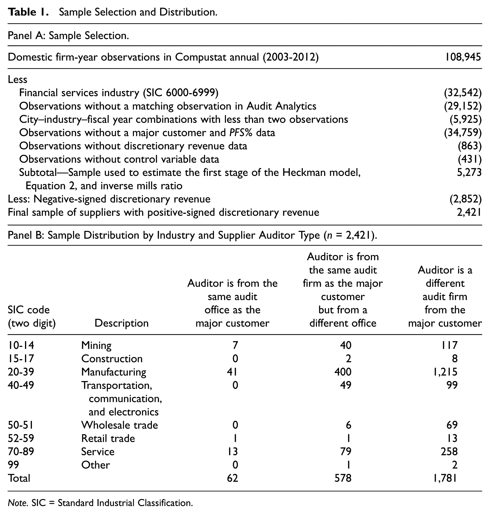
To examine our three predictions, we construct a sample of suppliers with major customers and with the necessary variables for our multivariate analysis (Table 1, Panel A). We start with all domestic companies from Compustat (2003-2012; 108,945 firm-year observations). 9 Next, we remove 32,542 observations from the financial services industry (Standard Industrial Classification [SIC] code 6000-6999) due to their dissimilar nature. To construct variables from Audit Analytics data, we remove 29,152 unmatched observations. To require a minimum of two observations per city–industry–fiscal year combination (Francis et al., 2005), we remove 5,925 observations. To ensure that each supplier has a major customer, and to compute PFS%, we remove 34,759 observations. To compute discretionary revenue and control variables, we remove 863 and 431 incomplete observations, respectively. So far, the sample has 5,273 firm-year observations, with positive-signed and negative-signed discretionary revenue, which we use to estimate the first stage of the Heckman model (Equation 2) for computing the inverse mills ratio (IMR). After restricting to positive-signed discretionary revenue, the final sample is 2,421 supplier firm-year observations. 10
Sample Selection and Distribution.
Note. SIC = Standard Industrial Classification.
To identify the supplier’s major customers, we use the Compustat Customer Segment Database as follows: Under FASB’s codification (ASC 280-10-50-42) and SEC Regulation S-K (17 CFR 229.101[c][1][vii]), if a customer accounts for at least 10% of a firm’s total sales revenue, the firm is required to report the name of the major customer and the total sales to the major customer in its Form 10-K filing. As the FASB and SEC requirements do not specify how to name the major customer, there is a lack of uniformity in naming the same major customer. Thus, we identify the major customers based on the procedure specified in Chen et al. (2014).
Panel B of Table 1 reports the number of supplier firm-year observations by industry and by auditor type (same audit office as the major customer, same audit firm as the major customer, and different audit firms from the major customer). Panel B reports that 62 firm-year observations (2.6%) have the same audit office as the major customer.
Analysis of Positive-Signed Discretionary Revenue
We are interested in investigating whether supplier positive-signed discretionary revenue is associated with the percentage of the major customer’s purchases when a supply chain auditor is engaged. We start our analysis by estimating positive-signed and negative-signed discretionary revenue, following Stubben (2010), as the difference between the actual change in uncollected revenues and the predicted change in uncollected revenues, estimated as the residual from

where it is the subscript for firm i in year t, ΔAR is the change in account receivables (rect) scaled by average total assets (at), ΔR is the change in revenue (salet– salet–1) scaled by average total assets, SIZE is the natural logarithm of total assets which proxies for a firm’s financial strength, AGE is the natural logarithm of the firm’s age in years which proxies for its stage in its life cycle, GRR is the industry median-adjusted growth rate in revenue (GRR_P if positive, GRR_N if negative), and GRM is the industry median-adjusted gross margin. Both GRR and GRM capture a firm’s operating performance relative to industry competitors. 11 AGE_SQ and GRM_SQ are the squared terms of the variables AGE and GRM, respectively. We estimate Equation 1 from all Compustat domestic companies (n = 108,945; Table 1) by industry (two-digit SIC) and year, with at least 10 observations per industry–year combination to obtain a robust estimate. To restrict revenue management to aggressive revenue management, we use positive-signed residuals (REV_DA > 0) from Equation 1. 12
A few points are worth noting. First, the model estimates unexpected accounts receivable growth; thus, the model likely does not estimate unusually high year-end cash sales. Rather, the model likely estimates accrual-based revenue management; thus, total revenue management is downward biased. Second, the model controls for the incentives of higher growth firms (Ertimur et al., 2003) by controlling for growth relative to competitors within the same industry.
The inferences from our sample of positive-signed discretionary revenue firms are potentially biased without controlling for self-selection bias. Firms self-select who are potentially younger, higher revenue growth firms with stronger incentives to meet or beat revenue benchmarks, compared with more mature firms who engage in more conservative revenue management. Product life cycle theory (Levitt, 1965) predicts that firms in the growth stage earn higher profit margins than their counterparts in the other stages. Firms that inflate revenue to manage earnings upward have higher profit margins (Plummer & Mest, 2001). However, among firms that have positive discretionary revenue, revenue targets and materiality constraints (rather than profit margin) likely determine the needed discretion to manage revenue. Thus, profit margin is an appropriate instrument, because it is likely associated with the sign of discretionary revenue but not with the magnitude.
We control for self-selection bias by the use of the Heckman (1979) two-stage model by including profit margin (PM) as a regressor in the first stage, which satisfies the exclusion restriction and is economically justifiable (Wooldridge, 2000). In the first stage, we estimate whether firms have positive-signed (vs. negative-signed) discretionary revenue, using PM and other firm characteristics (e.g., Callen, Robb, & Segal, 2008; Ertimur et al., 2003; Plummer & Mest, 2001; Reichelt & Wang, 2010) as regressors, in the following probit regression:

where RMS is equal to 1 if the residual from Equation 1 is positive, and 0 otherwise; REV_GWit–1 is lagged revenue growth rate; PM is operating income scaled by revenue; SIZE is the natural logarithm of total assets; MTB is the market-to-book ratio; EXP_HOMO is expense homogeneity; LOSS is equal to 1 if net income is negative, and 0 otherwise; OCF is operating cash flow scaled by lagged total assets; LEV is the ratio of total liabilities to total assets; ALTMAN is the Altman (1983) z score; and RET_DEV is the standard deviation of monthly stock return. Industry and year dummies are added to control for unobservable fixed effects. Appendix A reports the results of estimating Equation 2, n = 5,273, which shows that PM is positive and statistically associated with the likelihood of positive-signed discretionary revenue, and LOSS, OCF, and LEV are negatively associated.
In the second stage, we restrict the sample to firms with positive-signed discretionary revenue (n = 2,421), and we regress REV_DA > 0 on our variables of interest, control variables, and the inverse mills ratio (IMR; estimated from Equation 2). We test our first prediction by evaluating the association between the magnitude of positive-signed discretionary revenue and the percentage of purchases by the major customer when a supply chain auditor is engaged. We test the second and third predictions by the differential effects of interlocking directors and significant influence. We specify the following regression models:

and

Firm and year subscripts (it) are omitted for brevity.
We measure economic dependence of the major customer (on the supplier) by computing the major customer’s purchases from the supplier as a percentage of the major customer’s cost of goods sold (PFS%), following Hui et al. (2012). A major customer’s dependence is derived from the importance of the products they purchase from their supplier (Porter, 1980). PFS% measures the importance of the product to the major customer because a larger percentage of purchases from the supplier implies greater economic dependence. For instance, purchases by CCE from Coke comprise 45% of its cost of goods sold in 1999, which indicate greater economic dependence on Coke, compared with the purchases by Wal-Mart Stores, Inc., from Tyson Foods, Inc., in 2012 that only comprise 1%.
Returning to our discussion in Equation 3.1, Prediction 1 states that there is a positive association between positive-signed discretionary revenue and PFS% when a supply chain auditor is engaged. We construct the variable of interest, PFS%_AUDIT_O, which is defined as PFS% when the supplier engages the same office-level audit firm as their major customer, and 0 otherwise. 14 We expect a positive coefficient on PFS%_AUDIT_O. Relatedly, PFS%_AUDIT_NO is PFS% when the supplier engages the same audit firm as the major customer but from a different audit office, and 0 otherwise. PFS%_AUDIT_NF is PFS% when the supplier engages a different audit firm from the major customer, and 0 otherwise. To further support Prediction 1, we expect that the coefficient on PFS%_AUDIT_O is greater than that on PFS%_AUDIT_NO and PFS%_AUDIT_NF.
To test Prediction 2, whether the effect of Prediction 1 is more pronounced by the existence of interlocking directors with the major customer, we interact LOCK with PFS%_AUDIT_O, and test for whether the coefficient on PFS%_AUDIT_O × LOCK is positive. LOCK is an indicator variable equal to 1 when the supplier has at least one director who serves on the board of the major customer, and 0 otherwise. Director data are obtained from the Morningstar Historical Governance database (available through Audit Analytics) which identifies directors of publicly traded companies.
To test Prediction 3, whether the effect of Prediction 1 is more pronounced by the existence of significance influence over (or from) a major customer, we interact EQUITY with PFS%_AUDIT_O. EQUITY is an indicator variable equal to 1 when the supplier owns between 20% and 50% of the major customer or vice versa, and 0 otherwise. We test for whether the coefficient on PFS%_AUDIT_O × EQUITY is positive. We construct the variable EQUITY by hand-collecting ownership data from Form 10-K filings found on the SEC electronic data gathering, analysis, and retrieval system (EDGAR) website.
Equations 3.1 and 3.2 include variables of the supplier from prior studies that examine revenue overstatements (e.g., Callen et al., 2008). To control for auditor industry specialization, we follow Francis et al. (2005) and include the following indicator variables 15 : SPEC_F is equal to 1 when the auditor is the national industry specialist but not the city industry specialist. SPEC_O is equal to 1 when the auditor is the city industry specialist but not the national industry specialist. SPEC_FO is equal to 1 when the auditor is the industry specialist at both the national and city levels. We include the indicator variable, BIGN, to control for auditor size because prior studies (DeFond & Zhang, 2014) find that clients of Big N firms have lower levels of discretionary accruals. We include the indicator variable, ISSUE, to control for debt and equity issues, following Marquardt and Wiedman (2004) who find that firms that issue equity manage earnings upward by accelerating revenue recognition. We include the ratio of inventory to total assets, INV_ASSETS, to control for its association with auditor lawsuits (Stice, 1991). We include LOSS to control for incentives of loss firms to manage revenue down to meet future benchmarks. We include OCF because the cash burn rate (operating cash flow) of Internet firms is positively associated with grossed-up revenue (Bowen, Davis, & Rajgopal, 2002). We include LEV because firms approaching a debt covenant violation have incentives to make income-increasing discretionary accruals (DeFond & Jiambalvo, 1994). We include ALTMAN and RET_DEV to control for incentives from financial distress and business risk to inflate revenue (Callen et al., 2008). We include MTB to control for incentives for growth firms to inflate revenue (Ertimur et al., 2003). We include SIZE to control for supplier size effects. We include the inverse mills ratio, IMR, to control for self-selection bias. Industry and year dummies control for unobservable industry and year fixed effects.
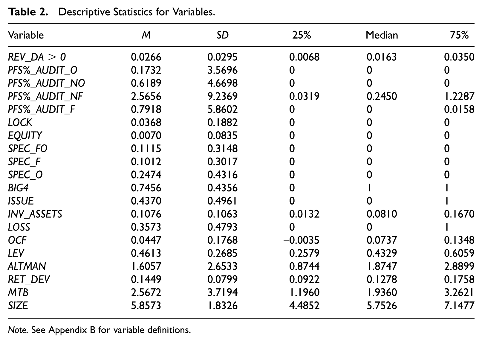
Table 2 reports the descriptive statistics of the aforementioned variables. 16 All continuous variables are winsorized at the 1st and 99th percentiles. The descriptive statistics of the control variables are comparable with those of prior studies, except for SPEC_F and SPEC_FO. Reichelt and Wang (2010) report lower mean values because their study requires at least a 10% greater market share for the industry specialist than the next competitor, whereas our variable definitions of SPEC_F and SPEC_FO only require that the industry specialist have the highest market share.
Descriptive Statistics for Variables.
Note. See Appendix B for variable definitions.
Untabulated Pearson’s correlation analysis shows that there is a positive and statistically significant correlation between REV_DA > 0 and PFS%_AUDIT_O, while there is no statistically significant correlation between REV_DA > 0 and PFS%_AUDIT_NO, and PFS%_AUDIT_NF, which provides preliminary support for Prediction 1.
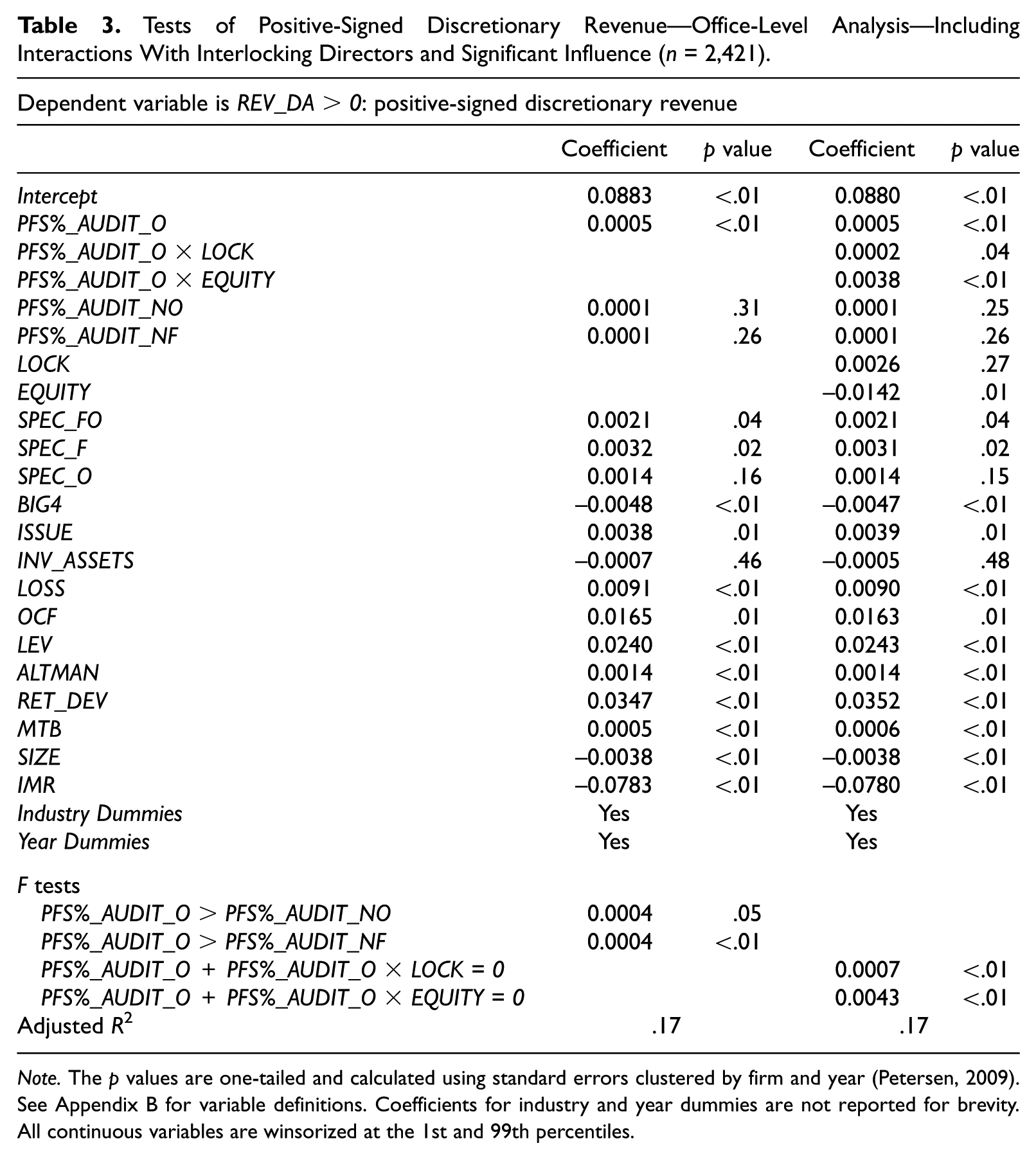
Table 3 reports the results of estimating Equations 3.1 and 3.2 with ordinary least squares (OLS) regression. For Equation 3.1, all of the coefficients on the control variables are significant at p < .10, except for the coefficients on SPEC_O and INV_ASSETS. The coefficient signs are consistent with the prior studies mentioned. The coefficient on IMR is negative and statistically significant, suggesting that self-selection bias is likely to be present in our sample (Wooldridge, 2000). If we include the instrument (PM) in estimating Equation 3.1, untabulated results show that the coefficient is positive and is not statistically different from zero (0.005, p = .79), suggesting that the exclusion restriction of the Heckman model is satisfied.
In support of Prediction 1, the coefficient on PFS%_AUDIT_O is positive and statistically significant. 17 A comparison of the coefficient on PFS%_AUDIT_O with PFS%_AUDIT_NO and with PFS%_AUDIT_NF indicates that the coefficient on PFS%_AUDIT_O is greater, thus providing further support for Prediction 1. Note that the coefficients on PFS%_AUDIT_NO and PFS%_AUDIT_NF are positive but statistically insignificant, suggesting that positive-signed discretionary revenue is not associated with PFS% when supply chain clients employ the same audit firm but different offices, or when they engage entirely different audit firms.
Tests of Positive-Signed Discretionary Revenue—Office-Level Analysis—Including Interactions With Interlocking Directors and Significant Influence (n = 2,421).
Note. The p values are one-tailed and calculated using standard errors clustered by firm and year (Petersen, 2009). See Appendix B for variable definitions. Coefficients for industry and year dummies are not reported for brevity. All continuous variables are winsorized at the 1st and 99th percentiles.
To measure the economic significance of our results, we compute mean marginal (to non-supply chain audit clients) positive-signed discretionary revenue as a proportion of total sales revenue (see Appendix C). For supplier clients with a supply chain auditor, mean marginal positive-signed discretionary revenue is 0.50% of total sales revenue. Using a benchmark materiality threshold of 0.50% of revenue, mean marginal discretionary revenue is material for supplier clients of supply chain auditors.
Next, for Equation 3.2, Table 3 reports that the coefficient on PFS%_AUDIT_O × LOCK is positive and significant, thus supporting Prediction 2. In addition, the coefficient on PFS%_AUDIT_O × EQUITY is positive, thus supporting Prediction 3. 18 The results are economically significant—Mean marginal positive-signed discretionary revenue for supplier clients with interlocking directors is 1.09% of sales revenue and 2.21% for clients with significant influence. These results suggest that the main results, which support Prediction 1, are moderated by interlocking directors and significant influence, and are economically significant.
Robustness Tests
Tests of Meeting or Beating Analysts’ Revenue Forecasts
As an alternative measure of revenue management, we investigate whether firms are more likely to meet or beat analysts’ revenue forecasts when they do not have sufficient premanaged revenues. As discussed, management has incentives to meet or beat analyst revenue forecasts (e.g., Edmonds et al., 2013). Following Davis, Soo, and Trompeter (2009), we employ a measure that identifies firms who meet or beat analysts’revenue forecasts with sufficient discretionary revenue. Specifically, we identify firms that meet or beat analysts’revenue forecasts with sufficient total revenue (discretionary revenue and nondiscretionary revenue) but insufficient nondiscretionary revenue. These identified firms presumably create sufficient discretionary revenue to meet or beat the revenue forecast target when nondiscretionary revenue is insufficient.
We calculate nondiscretionary revenue (NDREV) equal to actual revenue minus discretionary revenue (REV_DA > 0 times average assets). We then compute the adjusted revenue forecast error (ADJRFE) equal to NDREV minus the median analysts’ revenue forecast. 19 Next, to restrict our sample to firms with insufficient nondiscretionary revenue, we delete observations where ADJRFE > 0. MEET is equal to 1 if actual revenue (discretionary and nondiscretionary) meets or exceeds the median analysts’ revenue forecast, and 0 otherwise. Our sample size is reduced from 2,421 to 1,598 firm-year observations, primarily because we exclude observations with ADJRFE > 0 and without an analyst revenue forecast.
We test our three predictions by estimating the following probit models:
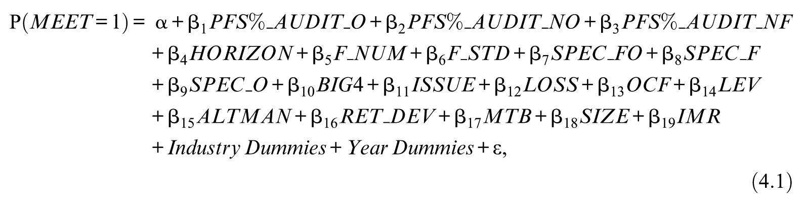
and

We include in Equations 4.1 and 4.2 control variables from Equations 3.1 and 3.2, and variables shown to affect forecast accuracy (Davis et al., 2009; Reichelt & Wang, 2010): HORIZON, F_NUM, and F_STD.
Table 4 reports the results of estimating Equations 4.1 and 4.2. The coefficient on PFS%_AUDIT_O is positive and significant, and the coefficient on PFS%_AUDIT_O is greater than that on PFS%_AUDIT_NO and PFS%_AUDIT_NF. The coefficients on PFS%_AUDIT_O × LOCK and PFS%_AUDIT_O × EQUITY are positive and significant. These results support Predictions 1, 2, and 3, and are consistent with our results from using positive-signed discretionary revenue.
Tests of Meeting or Beating Analysts’ Revenue Forecasts—Office-Level Analysis—Including Interactions With Interlocking Directors and Significant Influence (n = 1,598).
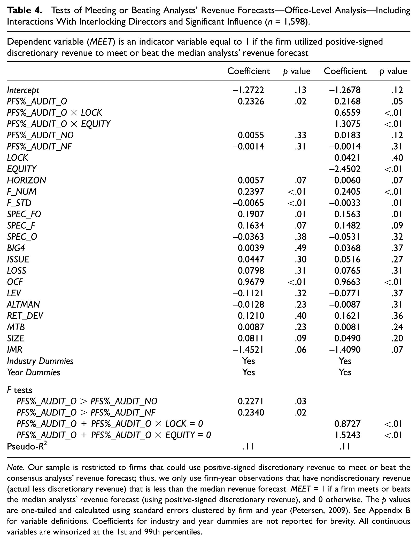
Note. Our sample is restricted to firms that could use positive-signed discretionary revenue to meet or beat the consensus analysts’ revenue forecast; thus, we only use firm-year observations that have nondiscretionary revenue (actual less discretionary revenue) that is less than the median revenue forecast. MEET = 1 if a firm meets or beats the median analysts’ revenue forecast (using positive-signed discretionary revenue), and 0 otherwise. The p values are one-tailed and calculated using standard errors clustered by firm and year (Petersen, 2009). See Appendix B for variable definitions. Coefficients for industry and year dummies are not reported for brevity. All continuous variables are winsorized at the 1st and 99th percentiles.
Other Discretionary Revenue Measures
To further evaluate the robustness of our empirical results, we employ three alternative discretionary revenue models 20 : First, we employ a measure following Caylor (2010) in which discretionary revenue is measured as the residual from estimating

where ΔARit is the change in accounts receivable scaled by lagged total assets (Ait–1), ΔREVit is the change in revenue, and ΔOCFit+1 is the change in next-year’s operating cash flow. We measure REV_DA > 0 as the positive-signed residual from Equation 5, and we estimate Equations 2, 3.1, and 3.2. Untabulated results indicate that our results hold for all three predictions.
In a second alternative model, we specify a modified version of Dechow and Dichev (2002) and measure discretionary revenue as the residual from estimating

where ΔAR is the change in accounts receivable, CFO is operating cash flow, and ΔREV is the change in revenue—where all variables are scaled by average total assets. We measure REV_DA > 0 as the positive residual from Equation 6. Untabulated results indicate that our results hold for Predictions 1 and 3, while Prediction 2 is not significant (p = .09).
In a third alternative model, we add to Equation 1 variables that are related to the supplier–customer relationship: PFS%, lagged major customer research and development (R&D) expenses (Raman & Shahrur, 2008), and major customer bargaining power—the ratio of market value of major customer firms to the market value of the supplier firm (Hui et al., 2012). We estimate REV_DA > 0 from the modified version of Equation 1. Untabulated results indicate that our results hold for Predictions 1 and 3, while Prediction 2 is not significant (p = .08).
Self-Selection Bias of Supply Chain Auditor Choice
The choice of a supply chain auditor is potentially self-selected, and the factors that determine auditor choice can influence the association between REV_DA > 0 and PFS%_AUDIT_O; thus, we control for self-selection bias of the supply chain auditor by employing a Heckman (1979) two-stage model in a manner similar to our main analysis. Specifically, we estimate the first stage from a probit model where the dependent variable is a supply chain auditor indicator variable. The control variables are lagged terms following prior studies (e.g., Ellis, Fee, & Thomas, 2012; Raman & Shahrur, 2008): auditor choice (major customer size less supplier size), a durable goods industry indicator (DGI), percentage of sales from major customers (PFM%), auditor office size (OSIZE), proprietary costs (mean industry R&D expense to sales ratio, mean industry advertising expense to total sales ratio, and Hirschman–Herfindahl index [HHI]), and client characteristics (client percentage of audit fees to audit firm, SIZE, return on sales, REV_GW, and LEV). We add an instrument, which satisfies the restriction exclusion, consisting of an indicator variable for whether the supply chain clients are in the same industry in the prior year. We estimate the inverse mills ratio from the first-stage probit model and include it in estimating Equations 3.1 and 3.2. Untabulated results indicate that our results hold for all three predictions.
Firm-Level Analysis
Potentially, the supply chain auditor is an audit firm-level phenomenon, rather than an audit office-level phenomenon, because major customer clients are more often audited in different offices by the same audit firm (Table 1, Panel B), and the loss of a major customer client affects the entire audit firm. To test this conjecture, we examine whether audit firm-level analysis is sufficient. We drop PFS%_AUDIT_O and PFS%_AUDIT_NO from Equation 3.1, and substitute PFS%_AUDIT_F which is PFS% when the supplier client employs the same audit firm as the major customer (ignoring offices), and 0 otherwise. Table 5 reports that the coefficients on PFS%_AUDIT_F and PFS%_AUDIT_NF are positive but not statistically significant, and they are not statistically different from each other. These findings suggest that supply chain auditors drive our main results.
Tests of Positive-Signed Discretionary Revenue—Firm-Level Analysis (n = 2,421).
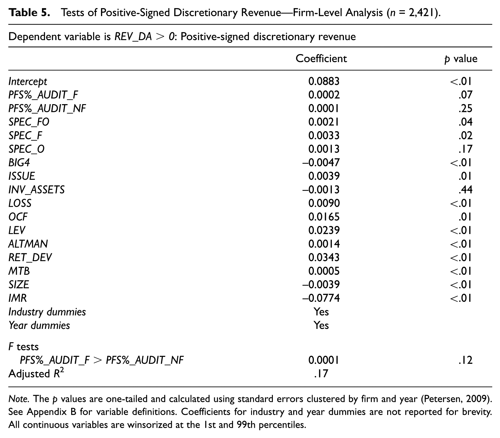
Note. The p values are one-tailed and calculated using standard errors clustered by firm and year (Petersen, 2009). See Appendix B for variable definitions. Coefficients for industry and year dummies are not reported for brevity. All continuous variables are winsorized at the 1st and 99th percentiles.
Supplier Auditor Switches Followed by Major Customer Auditor Switches
In the empirical predictions, we argue that the supply chain auditor is threatened by the loss of not just one client (the supplier) but two (the supplier and major customer). If this conjecture holds, then we should observe that the major customer is more likely to switch auditors in the current period, after the supplier switched auditors in the prior period, when the major customer is more economically dependent and aggressive revenue management is present. To test this conjecture, we restrict our sample to both positive- and negative-signed discretionary revenues (n = 4,565). We construct a logistic model where we regress an indicator variable for a current-period major customer auditor switch on two variables of interest: a prior-period supplier auditor-switch indicator variable (SUP_SWITCHt–1) interacted with PFS%_AUDIT_Ot and RMSt, and the interaction of SUP_SWITCHt–1× PFS%_AUDIT_Ot. The sum of the coefficients on these two interaction terms forms our test statistic, which we expect is positive. Control variables include sales to asset ratio, asset growth, accruals magnitude, SIZE, ROA, LOSS, LEV, MTB, and IMR. Untabulated results indicate that the sum of the coefficients on the two interaction terms is positive and significant (p = .02). This result supports our conjecture that supply chain auditors are threatened by the loss of not just the supplier client but also an economically dependent major customer when aggressive revenue management is present.
Aggressive Revenue Management and Supply Chain Auditor Switches
In the empirical predictions, we argue that engaging a supply chain auditor creates an economic bond between the supplier client and the auditor. To test the conjecture, we examine whether there is a lower likelihood of a supply chain auditor switch when prior-year aggressive revenue management is greater. We construct a probit model and restrict it to all auditor switches with positive-signed discretionary revenue (n = 62), where the dependent variable is an indicator variable for a current-year supply chain auditor switch. The variable of interest is lagged positive-signed discretionary revenue (REV_DA > 0t–1). We include lagged control variable terms for PFM%, OSIZE, DGI, ALTMAN, SIZE, LEV, HHI, REV_GW, and an indicator variable for whether the auditor and the supplier are in the same metropolitan statistical area (MSA). We find that the coefficient on REV_DA > 0t–1 is negative (p < .01), suggesting that clients are less likely to switch a supply chain auditor (than a nonsupply chain auditor) when aggressive revenue management is greater in the prior year. This result supports the conjecture that there is economic bonding between the supplier client and the supply chain auditor.
Other Robustness Tests
We employ several other robustness tests. First, we examine whether our results are robust to measuring aggressive revenue management as the likelihood of a revenue restatement that coincides with positive-signed discretionary revenue. A revenue restatement indicates that revenue was misstated in the first place, and the auditor erroneously issued an unqualified audit opinion (DeFond & Zhang, 2014). In untabulated results, we find that the coefficient on PFS%_AUDIT_O (p = .06) is positive, suggesting that a supplier client, who engages a supply chain auditor and has a more economically dependent major customer, is associated with a greater likelihood of a revenue restatement that coincides with positive-signed discretionary revenue. 21 Second, we decompose the variable of interest (PFS%_AUDIT_O) from Equation 3.1 into respective continuous and indicator variables. Specifically, we replace it with the interaction of PFS% and an indicator variable for supply chain auditors (AUDIT_O). We find similar results—The coefficient on PFS% × AUDIT_O is positive (0.0157, p = .04). Finally, we examine whether industry specialist auditors mediate our main results for Prediction 1. We add an interaction term (SPEC_FO × PFS%_AUDIT_O) to Equation 3.1, and we find that the coefficient sign is negative (p = .02). This result suggests that supply chain auditors, who are also joint national-office-level industry specialists, are less likely to tolerate aggressive revenue management when a more economically dependent major customer is present.
Conclusion
Our study examines whether supplier clients, who engage the same office-level auditor as their major customer, are associated with greater aggressive revenue management when the major customer is more economically dependent on the supplier. We also examine whether this association is moderated by interlocking directors and significant influence over or by major customers. Our article is motivated by the fact that there is little academic evidence about whether auditors are more tolerant of aggressive revenue management within the supply chain.
We measure aggressive revenue management as positive-signed discretionary revenue, while controlling for potential self-selection (Heckman, 1979) of supplier clients who aggressively manage revenue. We find that positive-signed discretionary revenue is positively associated with the percentage of purchases made by the major customer when a supply chain auditor is engaged. We fail to find a statistically significant association when the client supplier engages a different office-level auditor from that of the major customer or an entirely different audit firm. In addition, we find that our results are moderated by interlocking directors and by significant influence of the supplier client over or by the major customer. Our results are robust to several tests. Overall, our results imply that supply chain auditors are more tolerant of the supplier client’s aggressive revenue management when greater audit synergies are at risk. The presence of interlocking directors and significant influence contributes to the result.
One implication of our study is that retention of supply chain knowledge at the office level is more sensitive than industry knowledge. The loss of a supply chain client has a greater loss of knowledge than a client of an industry specialist, because there are fewer supply chain clients. 22 Thus, supply chain auditors seem to have stronger incentives to retain their supply chain clients.
A point worth noting is that only a small percentage of our supplier firm sample engages a supply chain auditor (2.6%). However, among the small percentage, the supply chain auditor constrains less aggressive revenue management. We acknowledge that discretionary revenues are only statistical estimates, and we cannot conclude they depart from GAAP. Nevertheless, regulators may find our results interesting for auditor inspection purposes and for monitoring registrants’ financial reporting (e.g., the Accounting Quality Model).
Footnotes
Appendix A
First-Stage Probit Regression of Revenue Management Sign on Profit Margin and Other Supplier Firm Characteristics (n = 5,273).

| Dependent variable (RMS) is an indicator variable equal to 1 if discretionary revenue is positive | ||
|---|---|---|
| Coefficient | p value | |
| Intercept | 0.3425 | .06 |
| REV_GWit –1 | –0.0207 | .67 |
|
|
|
|
| SIZEit | –0.0019 | .88 |
| MTBit | –0.0022 | .64 |
| EXP_HOMOit | –0.0357 | .81 |
|
|
|
|
|
|
|
|
|
|
|
|
| ALTMANit | –0.0026 | .79 |
| RET_DEVit | –0.0861 | .74 |
| Industry Dummies | Yes | |
| Year Dummies | Yes | |
| Pseudo-R2 | .02 | |
Note. The above probit regression estimates the first stage of the Heckman model by estimating the likelihood of positive-signed discretionary revenue (RMSit) from profit margin (PMit), and other supplier firm characteristics for firm i in year t. RMS is an indicator variable equal to 1 if discretionary revenue (the residual from Equation 1) is positive, and 0 otherwise. The independent variables are prior year’s revenue growth rate (REV_GWit–1), profit margin (PMit), client size (SIZEit), growth opportunities (MTBit), expense homogeneity (EXP_HOMOit), loss indicator (LOSSit), operating cash flow (OCFit), leverage (LEVit), Altman’s (1983) z score (ALTMANit), 12-month stock return volatility (RET_DEVit), industry fixed effects, and year fixed effects. See Appendix B for variable definitions. The exclusion restriction (Wooldridge, 2000) is satisfied because the coefficient on PM is positive and statistically significant, and if PM were included in the second stage (Equation 3.1), the coefficient (0.005) would not be statistically different from zero (p = .79).
Appendix B
Variable Definitions.
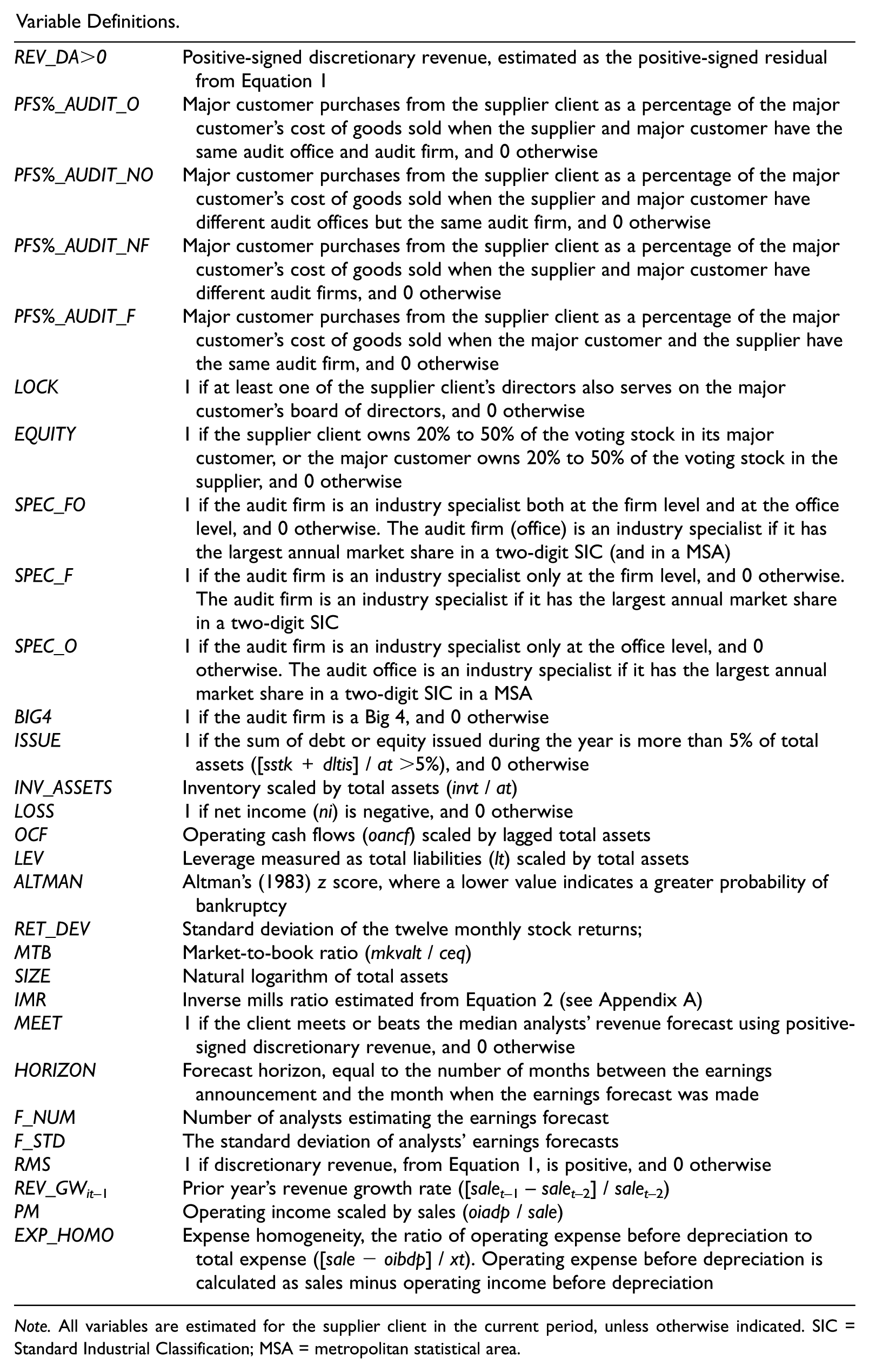
| REV_DA>0 | Positive-signed discretionary revenue, estimated as the positive-signed residual from Equation 1 |
| PFS%_AUDIT_O | Major customer purchases from the supplier client as a percentage of the major customer’s cost of goods sold when the supplier and major customer have the same audit office and audit firm, and 0 otherwise |
| PFS%_AUDIT_NO | Major customer purchases from the supplier client as a percentage of the major customer’s cost of goods sold when the supplier and major customer have different audit offices but the same audit firm, and 0 otherwise |
| PFS%_AUDIT_NF | Major customer purchases from the supplier client as a percentage of the major customer’s cost of goods sold when the supplier and major customer have different audit firms, and 0 otherwise |
| PFS%_AUDIT_F | Major customer purchases from the supplier client as a percentage of the major customer’s cost of goods sold when the major customer and the supplier have the same audit firm, and 0 otherwise |
| LOCK | 1 if at least one of the supplier client’s directors also serves on the major customer’s board of directors, and 0 otherwise |
| EQUITY | 1 if the supplier client owns 20% to 50% of the voting stock in its major customer, or the major customer owns 20% to 50% of the voting stock in the supplier, and 0 otherwise |
| SPEC_FO | 1 if the audit firm is an industry specialist both at the firm level and at the office level, and 0 otherwise. The audit firm (office) is an industry specialist if it has the largest annual market share in a two-digit SIC (and in a MSA) |
| SPEC_F | 1 if the audit firm is an industry specialist only at the firm level, and 0 otherwise. The audit firm is an industry specialist if it has the largest annual market share in a two-digit SIC |
| SPEC_O | 1 if the audit firm is an industry specialist only at the office level, and 0 otherwise. The audit office is an industry specialist if it has the largest annual market share in a two-digit SIC in a MSA |
| BIG4 | 1 if the audit firm is a Big 4, and 0 otherwise |
| ISSUE | 1 if the sum of debt or equity issued during the year is more than 5% of total assets ([sstk+dltis] / at >5%), and 0 otherwise |
| INV_ASSETS | Inventory scaled by total assets (invt / at) |
| LOSS | 1 if net income (ni) is negative, and 0 otherwise |
| OCF | Operating cash flows (oancf) scaled by lagged total assets |
| LEV | Leverage measured as total liabilities (lt) scaled by total assets |
| ALTMAN | Altman’s (1983) z score, where a lower value indicates a greater probability of bankruptcy |
| RET_DEV | Standard deviation of the twelve monthly stock returns; |
| MTB | Market-to-book ratio (mkvalt / ceq) |
| SIZE | Natural logarithm of total assets |
| IMR | Inverse mills ratio estimated from Equation 2 (see Appendix A) |
| MEET | 1 if the client meets or beats the median analysts’ revenue forecast using positive-signed discretionary revenue, and 0 otherwise |
| HORIZON | Forecast horizon, equal to the number of months between the earnings announcement and the month when the earnings forecast was made |
| F_NUM | Number of analysts estimating the earnings forecast |
| F_STD | The standard deviation of analysts’ earnings forecasts |
| RMS | 1 if discretionary revenue, from Equation 1, is positive, and 0 otherwise |
| REV_GWit –1 | Prior year’s revenue growth rate ([salet–1–salet–2] / salet–2) |
| PM | Operating income scaled by sales (oiadp / sale) |
| EXP_HOMO | Expense homogeneity, the ratio of operating expense before depreciation to total expense ([sale−oibdp] / xt). Operating expense before depreciation is calculated as sales minus operating income before depreciation |
Note. All variables are estimated for the supplier client in the current period, unless otherwise indicated. SIC = Standard Industrial Classification; MSA = metropolitan statistical area.
Appendix C
Acknowledgements
We gratefully acknowledge the comments and suggestions of Carolyn Callahan, Agnes Cheng, Jong-Hag Choi, Larry Crumbley, Patricia Dechow, Harry Evans, Norman Massel, Zabihollah Rezaee, Jared Soileau, Janet Souza, Paul Tanyi, and Joseph Hongbo Zhang; the workshop participants at Drexel University, National Taipei University, and the University of Memphis; and participants at the 2013 European Accounting Association Annual Congress. Kenneth Reichelt acknowledges financial support from the Louisiana State University E. J. Ourso College of Business.
Declaration of Conflicting Interests
The author(s) declared no potential conflicts of interest with respect to the research, authorship, and/or publication of this article.
Funding
The author(s) received no financial support for the research, authorship, and/or publication of this article.