
Abstract
Management research increasingly recognizes omitted variables as a primary source of endogeneity that can induce bias in empirical estimation. Methodological scholarship on the topic overwhelmingly advocates for empirical researchers to employ two-stage instrumental variable modeling, a recommendation we approach with trepidation given the challenges associated with this analytic procedure. Over the course of two studies, we leverage a statistical technique called the impact threshold of a confounding variable (ITCV) to better conceptualize what types of omitted variables might actually bias causal inference and whether they have appeared to do so in published management research. In Study 1, we apply the ITCV to published studies and find that a majority of the causal inference is unlikely biased from omitted variables. In Study 2, we respecify an influential simulation on endogeneity and determine that only the most pervasive omitted variables appear to substantively impact causal inference. Our simulation also reveals that only the strongest instruments (perhaps unrealistically strong) attenuate bias in meaningful ways. Taken together, we offer guidelines for how scholars can conceptualize omitted variables in their research, provide a practical approach that balances the tradeoffs associated with instrumental variable models, and comprehensively describe how to implement the ITCV technique.
Keywords
“Omitted variables bias is said to be the most commonly encountered problem in social behavioral sciences.”
The detrimental influence of omitted variables in empirical analyses has been recognized in management research for decades (Bascle, 2008; Hill, Johnson, Greco, O’Boyle, & Walter, 2021; Shaver, 1998). Omitted variables refer to factors that influence the dependent variable of interest but are not included in the analytic model. These variables are problematic for empirical estimation when they also influence a focal independent covariate, thus confounding the relationship between the focal independent and dependent variables and causing omitted variable bias (Frank, 2000; Semadeni, Withers, & Certo, 2014; Wooldridge, 2010). Although confounding omitted variables can create bias in empirical research regardless of discipline, they are particularly deleterious for management research since the literature is “fundamentally predicated on the idea that management’s decisions are endogenous . . . if not, managerial decision-making is not strategic; it is superfluous” (Hamilton & Nickerson, 2003: 51).
The role of omitted variable bias in management research is embedded within broader work on endogeneity, which paints a gloomy picture for empirical researchers (Hill et al., 2021). Semadeni et al. (2014: 1071) suggest that endogeneity can have “pernicious effects” even when the error term has a weak correlation with predictors. Scholars indicate an error term that is correlated with the independent and dependent variables can create estimation biases almost irrespective of the magnitude of the correlation (Certo, Busenbark, Woo, & Semadeni, 2016; Hamilton & Nickerson, 2003; Semadeni et al., 2014). Compounding this problem is the fact that one of the most popular techniques to attenuate bias from endogeneity—instrumental variable modeling—can undermine inference (Larcker & Rusticus, 2010; Semadeni et al., 2014).
While the message of this literature on endogeneity is clear and beneficial, extant methodological research does not isolate the influence of omitted variables as a specific source of endogeneity or offer guidance on how to identify when an omitted variable may create estimation issues. This is troublesome because scholars are often primed to consider that there is nearly always a relevant omitted variable that likely biases statistical models (Hamilton & Nickerson, 2003). Yet models that do not specifically address omitted variables may at times be more appropriate than those that work to attenuate bias, especially given the tradeoffs associated with instrumental variable regression and the efficiency of OLS models (Kennedy, 2008; Semadeni et al., 2014; Wooldridge, 2010). Accordingly, the purpose of this study is to examine the following questions: (1) To what extent is omitted variable bias an issue in management research? (2) Can scholars quantify the effect of omitted variables? and (3) When should scholars seek to address omitted variables in their empirical estimation?
To address these questions, we conduct two studies that leverage an emerging statistical technique referred to as the impact threshold of a confounding variable (ITCV). The ITCV is focused on potential bias in causal inferences, or the ability to “draw conclusions about causal relationships between dependent and independent variables from statistical models using data from observational studies” (Pan & Frank, 2003: 315). This procedure delineates how correlated a confounding (used interchangeably with omitted) variable would have to be with the independent and dependent variables for the statistical inference to change (Frank, 2000; Frank, Maroulis, Duong, & Kelcey, 2013). The ITCV therefore shifts the concern from whether an empirical relationship is biased due to an omitted variable to “how much bias must be present to invalidate an inference” (Frank et al., 2013: 448). Scholars suggest that relatively high values of the ITCV indicate there is unlikely a biased causal inference in a study, whereas lower ITCV scores imply that an omitted variable bias is a potentially pressing concern (Harrison, Boivie, Sharp, & Gentry, 2018; Hill, Recendes, & Ridge, 2019; Hubbard, Christensen, & Graffin, 2017).
In Study 1, we conduct a content analysis of all empirical articles published in the Academy of Management Journal (AMJ), Journal of Applied Psychology (JAP), Journal of Management (JOM), and Strategic Management Journal (SMJ) in 2017 to calculate the ITCV values associated with each focal relationship in the studies. 1 After estimating the ITCV values, we look across the articles to approximate how likely it is for causal inferences to have been invalidated by an omitted variable. The outcomes associated with our examination are informative. Out of 382 causal relationships tested in empirical articles in these journals that do not explicitly account for potential omitted variables, approximately 15% to 25% of them were potentially biased from an omitted factor using notably stringent and rigid interpretations of the ITCV (Larcker & Rusticus, 2010; Pan & Frank, 2003). Almost no relationships featured biased causal inference if we consider a more realistic interpretation of the technique.
In Study 2, we use the values from our content analysis to perform a simulation that extends methodological scholarship on endogeneity (e.g., Certo et al., 2016; Larcker & Rusticus, 2010; Semadeni et al., 2014). In particular, we respecify one of the influential simulations on the topic (i.e., Semadeni et al., 2014), such that we focus on the potential biases induced by omitted variables rather than all sources of endogeneity simultaneously. We examine the distribution of beta coefficients across 1,000 simulation iterations per condition. Stated differently, we estimate the coefficient for each simulation condition 1,000 times, and then we depict the distribution of that coefficient across the 1,000 iterations. This represents one advantage of simulations since parameter estimates are intended to help scholars determine a sampling distribution of a relationship (Cohen, Cohen, West, & Aiken, 2003; Goldfarb & King, 2016; Schwab & Starbuck, 2017). Our simulations reveal that models begin to exhibit bias (i.e., OLS produced statistically significantly different estimates than specified) only when omitted variables feature higher confounding correlations than exist in most studies in our content analysis. Even when the omitted variable(s) features such high correlations, the causal inference from the outcomes remains almost unchanged. Our simulations also show that biased regression models estimate coefficients more similar to correctly specified models than do the two-stage instrumental variable techniques often employed to attenuate bias in most conditions.
This study offers at least two important implications for empirical management research. First, we extend the relatively nascent knowledge about the ITCV. To date, only a few studies published in management incorporate the ITCV in their empirical analyses, and to our knowledge, no studies have done so prior to 2017 (e.g., Busenbark, Lange, & Certo, 2017; Harrison et al., 2018; Hill et al., 2019; Hubbard et al., 2017). Although a search for management research that includes the ITCV populates several working papers and manuscripts invited for resubmission, there is certainly no consensus about how to use it, when it is appropriate, and when it is misleading. Before delving into our two interrelated studies, we thus offer comprehensive guidelines for how to appropriately incorporate and interpret the ITCV.
Second, we help scholars begin to think through what omitted variables may need to look like in order to represent problematic confounds for any specific relationship of interest. We certainly recognize the potentially disastrous effects omitted variables can have on accurate parameter estimation and causal inference (Hamilton & Nickerson, 2003; Semadeni et al., 2014). At the same time, we also acknowledge that most empirical modeling in management research (and the broader social sciences for that matter) deals with causal inference rather than seeking to uncover exact parameter estimates or coefficients (Cohen et al., 2003; Frank, 2000; Wooldridge, 2010). We therefore step back from the idea that virtually all omitted variables induce substantive issues in analytical estimation (Certo et al., 2016; Semadeni et al., 2014), and we instead adopt an approach that recognizes not all omitted variables are problematic. One implication from this study, then, is to aid researchers in thinking more comprehensively about what omitted variables may exist and whether they create estimation issues.
Omitted Variable Bias in Management Research
Omitted Variable Bias as a Source of Endogeneity
“When there is correlation between a regressor [independent variable] and the error term, that regressor is said to be endogenous; when no such correlation exists the regressor is said to be exogenous” (Kennedy, 2008: 139, emphasis in the original). Endogeneity biases results, producing incorrect coefficient estimates and predicting statistical significance more or less often than what actually exists (Bascle, 2008; Hill et al., 2021). Although the purpose of this study is not to exhaustively demonstrate how and why endogeneity can bias results, we reiterate the four potential sources of endogeneity that Kennedy (2008) describes: (1) measurement error, (2) autoregression, (3) simultaneous causality, and (4) omitted variables.
We focus this study on omitted variables. Although we realize all sources of endogeneity are potentially problematic, omitted variables bias represents one of the most pervasive issues for management researchers (Hamilton & Nickerson, 2003; Hill et al., 2021). To this point, we examined all published studies in AMJ, JOM, and SMJ from the years 2000-2018 and found that omitted variables were discussed in the context of potential empirical bias more so than any other source of endogeneity. In fact, empirical research published in these journals highlighted omitted variables in the context of bias from endogeneity approximately three times as often as any other source, including autocorrelation, which is often discussed in the context of panel data and repeated observations over time. 2
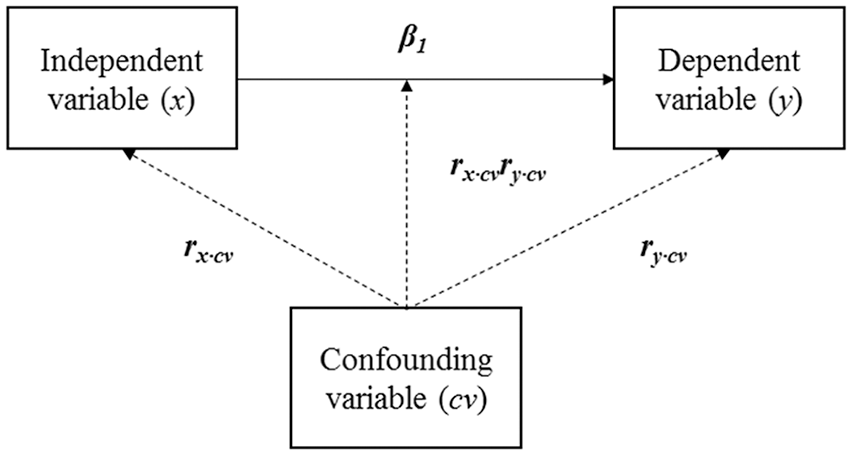
Omitted variables can influence the relationship between independent and dependent variables by assigning undue variance to the independent variable such that its coefficient is larger than in the absence of omitted variables (Hamilton & Nickerson, 2003; Kennedy, 2008). We depict these relationships between focal variables and an omitted variable in Figure 1, where β1 represents the estimated relationship between the independent variable (x) and the dependent variable (y) from a regression model (such as OLS). In the absence of a confounding variable, β1 is an accurate reflection of the correlation between x and y. In the presence of a confounding variable, however, β1 partially represents the correlation between x and y and partially reflects the relationship between the omitted variable and y. The extent to which β1 captures some of the correlation with the confounding variable is referred to as bias in the coefficient. In some cases, the correlation between the confounding variable and x and/or y is low enough that β1 reflects only trivial bias and does not change causal inference. In more extreme cases when the confounding variable explains all (or most) of the correlation between x and y, β1 is spurious and causal inference is biased (Kennedy, 2008; Wooldridge, 2010).
Relationships Between Independent, Dependent, and Confounding Variables
Techniques to Minimize the Bias from Omitted Variables
Given the potential for omitted variable bias in management research (Bascle, 2008; Hamilton & Nickerson, 2003), scholars have explored analytic techniques to reduce corresponding contamination in empirical models (Semadeni et al., 2014). The most prevalent technique involves instrumental variables and a sequence of equations (Kennedy, 2008). Instrumental variables are parameters that are correlated with the independent variable but not any confounding variables (Kennedy, 2008; Larcker & Rusticus, 2010). Scholars can use instrumental variables in two-step procedures that adjust parameters and the error term in a way that attenuates bias stemming from the omitted variable (Wooldridge, 2010).
Despite the intuitive nature of instrumental variable techniques, there are at least two important issues associated with such procedures. First, these techniques are inefficient compared to conventional modeling like OLS regression (Greene, 2018; Kennedy, 2008; Wooldridge, 2010). Inefficiency refers to the idea that the model is less likely to detect a nonzero relationship than may actually exist owing to inflated standard errors. Kennedy (2008: 149) suggests this occurs because the empirical estimator loses a great deal of “information” about the independent variable by predicting it as a function of instruments. While good instruments provide an unbiased estimate, they limit the variance (and thus covariance) of the independent variable. Scholars are therefore cautioned to consider the prevalence of bias before subjecting their models to this potential error (Baum, 2006; Kennedy, 2008), a practice that is seemingly rarely employed in published scholarship and thus represents the impetus for our research.
Second, irrelevant or endogenous instruments can introduce more bias in the model than what would have otherwise existed in the absence of instrumental variable techniques (Semadeni et al., 2014; Stock, Wright, & Yogo, 2002). Irrelevant instruments refer to those that do not have strong predictive power for the independent variable of interest (Stock et al., 2002), so they produce biased results since they do not accurately estimate the independent variable and thus induce measurement error (Kennedy, 2008). Endogenous instruments refer to those that are also correlated with the confounding variable (or the structural error term more broadly) and thus produce a biased estimate of the independent variable (Kennedy, 2008; Semadeni et al., 2014). Semadeni et al. (2014) demonstrate through simulations that even slightly endogenous instruments create bias where none otherwise exists.
Although scholars are repeatedly cautioned about the unintended and unfavorable consequences of two-step instrumental variable procedures (Certo et al., 2016; Kennedy, 2008; Semadeni et al., 2014), omitted variable bias remains a pervasive issue on the minds of authors, reviewers, and editors (Bettis, Gambardella, Helfat, & Mitchell, 2014; Hill et al., 2021). Over seven times as many articles published in AMJ, JOM, and SMJ mention and adjust for endogeneity (or omitted variables) in 2016 or 2017 than did in 2000 to 2003, and the portion of articles that consider omitted variables has more than doubled since 2011. It is clear that omitted variable bias is top-of-mind and that scholars are required to consider it sometime during or before the publication process. One central imperative of the present study, then, is to further explore whether omitted variables are a pervasive issue for management research and what characteristics of omitted variables create estimation issues.
ITCV
Overview of the ITCV
The ITCV is an index developed to quantify the impact of an omitted variable on parameter estimation and help scholars consider whether confounding factors might exist in their data. More specifically, the ITCV calculates the minimum correlations necessary to alter a causal inference of a regression coefficient due to an explanatory variable that is not included in the model (Frank, 2000; Frank et al., 2013). As Frank (2000: 150) describes, the purpose of the ITCV is “to calculate a single valued threshold at which the impact of the confound would be great enough to alter an inference with regard to a regression coefficient.” Scholars can use the ITCV equation as a sensitivity analysis to determine the correlation values at which the estimate for the independent variable becomes sufficiently high enough to be considered “not zero” based on a specified p value (see Frank, 2000: 153, Equation 3).
Figure 1 helps demonstrate the practical application and interpretation of the ITCV. In Figure 1, β1 represents the parameter estimate for the independent variable. Management scholars tend to interpret the usefulness of β1 based on whether or not it is likely nonzero (i.e., the causal inference), which often involves examining the p value and/or confidence interval of the coefficient (Schwab & Starbuck, 2017). If the confounding variable (cv) is correlated highly enough with the independent variable (rx,cv) and the dependent variable (ry,cv), β1 may reflect a nonzero relationship between x and y owing to the correlations between cv and the independent and dependent variables (rx,cvry,cv) instead of any actual correlation between x and y. This scenario represents biased causal inference.
The purpose of the ITCV is to provide a value for the correlation between the omitted variable and both focal variables (rx,cvry,cv) at which a nonzero β1 is actually caused by the confounding variable instead of the relationship between x and y. For instance, an ITCV value of 0.20 means an omitted variable would need to have an average partial correlation with the independent and dependent variables at a minimum of 0.20 to invalidate the causal inference. Higher ITCV scores indicate an omitted variable would have to possess a higher correlation, which suggests it is less likely to bias inferences.
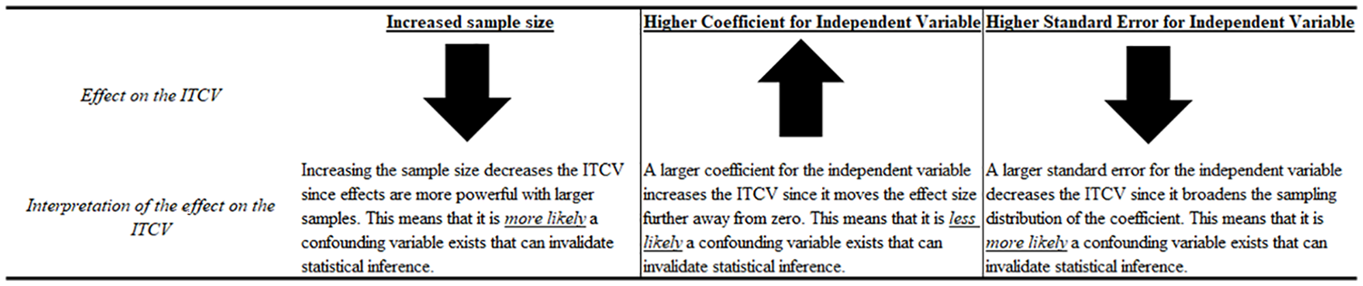
We provide Figure 2 to depict the three elements that influence the size of the ITCV at any given p value—the sample size, the coefficient for the independent variable, and the standard error of the independent variable (Frank, 2000). All else equal, changing any of these three elements will alter the ITCV values. For instance, increasing the sample size to test a specific relationship will decrease the ITCV value because larger sample sizes confer more accuracy with relationships and make correlations more salient. When the sample size is larger, an omitted variable with a lower correlation is simply more influential. Conversely, a larger absolute coefficient for the independent variable increases the ITCV since the estimated relationship is more differentiated from zero. Similarly, increasing the standard error of a parameter estimate speaks to the accuracy of the sampling distribution of coefficients (smaller standard errors translate to more accuracy) and decreases the ITCV. 3
Influence of Different Inputs on the ITCV
Scholars have also endeavored to build on the ITCV in order to develop a similar technique with identical inputs that works to address situations when the ITCV is less appropriate (we discuss the limitations of the ITCV in the coming sections). Although management scholars have referred to such an interpretation as the ITCV because the inputs for the calculations are identical to those for the correlation-based value, Frank et al. (forthcoming) refer to this approach as the robustness of inference to replacement (RIR). The RIR provides insight into the percentage of a parameter estimate that would need to be biased in order to invalidate causal inference (Xu & Frank, forthcoming). Although a comprehensive review of the RIR is beyond the scope of our research, Appendix 1 details essential elements of the technique.
Since the ITCV (and the RIR for that matter) is concerned with omitted variables that may shift estimated relationships further from zero, the directionality of the correlations is an integral element of the technique. If the relationship between x and y is positive, the product of the correlations between those two focal variables and the omitted variable must be positive to induce bias (i.e., both must be positive or negative, but not opposite). The inverse is true if the substantive relationship is negative (i.e., the omitted variable must be negatively correlated with one of the variables and positively correlated with the other) (Frank, 2000; Frank et al., 2013). We summarize the role of directionality in Appendix 2.
Interpreting the ITCV
Larcker and Rusticus (2010) were among the first scholars to incorporate and interpret the ITCV in business research. In their models, they found that the ITCV value was 0.167, meaning an omitted variable would have to possess an average correlation of at least 0.167 with both bid-ask spread (the independent variable) and disclosure quality (the dependent variable) for the estimated nonzero relationship between the two to actually not be different from zero. 4 As Larcker and Rusticus (2010: 202) argue in their study, scholars “need to develop a benchmark for the size of likely correlations involving the unobserved confounding variable. While, by definition, we do not have the unobservable confounding variable, we do have other control variables.” These scholars then describe how control variables represent an appropriate benchmark against which to determine whether the ITCV value may reasonably reflect relationships with a confounder.
The management scholars who have incorporated the ITCV have followed the interpretation Larcker and Rusticus (2010) propose by using the control variables (i.e., covariates) in their studies as proxies for the potential correlations of an omitted variable (Busenbark et al., 2017; Gamache, McNamara, Graffin, Kiley, Haleblian, & Devers, 2019; Harrison et al., 2018; Hubbard et al., 2017; Oliver, Krause, Busenbark, & Kalm, 2018). These researchers suggest that if no (or very few) measured covariates possess correlations higher than the ITCV value, it is unlikely an omitted variable would feature such a correlation. For instance, Hubbard et al. (2017: 2262) contend, “. . . it would take a correlated omitted variable with an impact nearly as large as the strongest variable in this model to overturn the results. Assuming that we have a reasonable set of control variables, this suggests that the results are not likely driven by a correlated omitted variable.” Similarly, Oliver et al. (2018: 122) uncover an ITCV of 0.25 and argue, “given the maximum correlation between our control variables and our dependent variable and/or independent variables is 0.09, it is hard to imagine an omitted variable with a correlation greater than the necessary 0.25.”
Although a majority of the research that has leveraged the ITCV focuses on control variables with a correlation between the independent and dependent variables at a value that must exceed the ITCV threshold as a reasonable approach (Gamache & McNamara, 2019; Oliver et al., 2018), it is important to highlight that the ITCV represents the path coefficient of a relationship that reflects the multiplication of two correlations. Put a different way, the most accurate means to interpret the ITCV involves multiplying the correlation between the control/independent variable by the correlation between the control/dependent variable and determining if the square root of that correlation is greater than the ITCV value. Figure 1 helps illustrate this point; if we substitute a control variable for the confounding variable (cv), any control with rx,cvry,cv (the square root of the multiplication of the two correlations) greater than the ITCV represents a potentially problematic proxy.
Perhaps following the lead of Larcker and Rusticus (2010), the overwhelming majority of research that seeks to interpret the ITCV tends to examine the zero-order correlations between control variables as such proxies. The ITCV, however, represents the requisite partial correlations with a confounding variable to invalidate an inference (Frank, 2000; Frank et al., 2008). Stated differently, the ITCV calculates the threshold correlations with a confounding variable after partialling out (i.e., removing) all the shared covariance with all the other covariates in the model. Accordingly, partial correlations are typically notably lower than zero-order correlations (see Cohen et al., 2003: Section 3.3 for formulas and discussions of partial correlations). This means interpreting the ITCV against the zero-order correlations typically featured in a “descriptive statistics” table is incredibly conservative since all of the correlations with control variables featured in the table are surely larger than their partial versions.
Nevertheless, it remains difficult to adjust the zero-order correlations from such a table to partial correlations because scholars typically do not report the requisite information to make the post hoc transformations. For this reason, our results in Study 1 feature the conservative zero-order correlations from published studies. We therefore argue it is incumbent on researchers seeking to interpret the ITCV to at least note the highest partial correlations in their study against which to compare the ITCV value. Although we recognize space is at a premium in the publication process and may not allow for a partial correlation matrix, scholars can minimally indicate the variables with the strongest partial correlations in the context of their ITCV analyses.
Limitations of the ITCV
Notwithstanding the merits of the ITCV, there remain several empirical and conceptual limitations. Perhaps most notably, it is important to highlight that the ITCV is useful to examine the causal inference and statistical significance of relationships between independent and dependent variables, but it does not address inaccuracies of the parameter estimate itself (Frank, 2000; Frank et al., 2013; Larcker & Rusticus, 2010). Indeed, the ITCV represents a threshold correlation at which a statistical inference regarding a hypothesized relationship estimated from a model (at any given specified p value) is invalidated if the correlation with that omitted variable is higher than the threshold. The actual value and practical interpretation of the coefficient, however, may change quite drastically if an omitted variable exists with a correlation lower than the threshold value even if the statistical inference remains the same. The ITCV thus helps provide sensitivity analyses for determining whether a coefficient is reasonably nonzero, but it does not afford scholars much guidance in terms of practically interpreting their models. 5
Further, and despite the prevalent use of such control variable-based interpretations of the ITCV, they are not infallible. It is indeed possible that an omitted variable exists that exhibits a correlation with the independent and dependent variables at values greater than control covariates included in any given study. There is also a fair degree of subjectivity in how scholars choose to incorporate control variables as comparisons for a potential omitted variable. As we highlight in this section, most scholars consider whether there are at least one or two controls with correlation properties that exceed the ITCV.
The appropriateness of the ITCV also depends on the nature of the empirical estimation procedure and corresponding data. As Frank (2000) describes, the ITCV is unable to provide much insight for estimates from logit or probit models. The ITCV is, however, appropriate for other models that use maximum likelihood estimation, such as panel data models (e.g., fixed effects or random effects), tobit models, weighted regression, Poisson models, and many other similar techniques. The ITCV is also currently unable to address interaction terms because the marginal effects of the relationships are contingent on the values of the lower order constituents. 6 Some preliminary research suggests omitted variable bias may be remarkably less pronounced in interaction terms than conventional variables (Bun & Harrison, 2019), though, so it is possible that the ITCV is superfluous in these scenarios.
Illustrating the ITCV in Management Research
The ITCV is a quite accessible tool that management scholars have begun to adopt over the course of the past several years (e.g., Busenbark et al., 2017; Harrison et al., 2018; Hill et al., 2019; Hubbard et al., 2017). For instance, strategy scholars have incorporated the ITCV in their studies to examine how an omitted variable may (or may not) overturn the relationship between foreshadowing acquisitions and analyst assessments (Busenbark et al., 2017), CSR investments and CEO dismissal (Hubbard et al., 2017), media coverage and director exit (Harrison et al., 2018), board chair orientations following the appointment of a female CEO (Oliver et al., 2018), and CEO characteristics and competitive attacks (Hill et al., 2019), among others.
Although more micro-oriented research has yet to adopt the ITCV to our knowledge, it could prove quite helpful in this domain as well. This is perhaps particularly the case for organizational behavior studies that involve samples derived from time-limited settings, such as experience sampling methods (ESM) studies (Gabriel et al., 2019), although the value of the ITCV is certainly not confined to such settings. In micro-oriented management scholarship, researchers are often constrained in terms of the number of variables they can collect, so it is quite costly to secure more data after the initial process (Atinc, Simmering, & Kroll, 2012; Gabriel et al., 2019). Indeed, a great deal of this research (e.g., job satisfaction, leader-member exchanges, voice, stress, etc.) examines data collected via survey or nonrandomized experiment (Judge, Locke, Durham, & Kluger, 1998; Matta, Scott, Koopman, & Conlon, 2015; Van Dyne & LePine, 1998). Accordingly, employing tenable two-stage models is challenging because locating viable instruments often requires a variety of variables at the researcher’s disposal. Organizational behavior scholars concerned about omitted variable bias could thus consult the ITCV and interpret it with the controls included in their studies, thereby perhaps ameliorating the necessity for infeasible instrumental variable models.
ITCV decision tree
In Figure 3, we provide a decision tree that helps explicate when the ITCV is appropriate, when to consider alternative techniques, and under what conditions scholars might suggest the causal inference of their relationship is unlikely biased from omitted variables. The purpose of Figure 3 is not to necessarily provide an exhaustive overview of the ITCV but rather to help scholars think through whether and when the ITCV may prove insightful.

Decision Tree of When to Employ the ITCV
As we show in the decision tree in Figure 3, the first step in applying the ITCV involves considering whether confounding variables may exist in a given relationship. Most relationships management scholars study are endogenous and thus could feature a problematic omitted variable (Hamilton & Nickerson, 2003; Semadeni et al., 2014), but this is not always the case (e.g., political ideologies, birth order, personality traits). If there is a potential for omitted variable bias due to confounding variables, however, in Figure 3 we suggest scholars should then consider the nature of their data. Specifically, if the dependent variable is binary or the parameters are interaction terms, we submit that the ITCV is currently inappropriate. The RIR may prove useful in such circumstances, and it may provide more insight about the treatment effects underlying binary independent variables (Xu & Frank, forthcoming; Xu, Frank, Maroulis, & Rosenberg, 2019).
Finally, in Figure 3, we provide some guidance as to how management researchers might consider the values derived from the ITCV in situations when the technique is appropriate. Specifically, we encourage scholars to interpret the output against existing control variables in their study, taking particular care to ensure to compare the ITCV values against partial correlations of control variables with the independent and dependent variables. If it appears as though there are no control variables with correlations that exceed the ITCV value, scholars may suggest it is unnecessary to employ instrumental variable models. It is imperative to reiterate here that the ITCV does not absolve researchers from addressing omitted variable bias, but rather it provides some insight as to the extent of potential bias (Frank, 2000). It is, however, quite appropriate to question whether the tradeoffs associated with instrumental variables are beneficial in such a circumstance.
ITCV illustration study
We now turn our attention to illustrating precisely how to calculate the ITCV. Specifically, we examine the empirical estimation and descriptive statistics from Gamache and McNamara (2019) to demonstrate how to compute and interpret the ITCV. We provide a step-by-step guide of how to use existing data and empirical analyses to compute the ITCV in the Stata command that Xu et al. (2019) created, although scholars can perform these same calculations using R code or the applications that are detailed on the website we link.
Gamache and McNamara (2019) theorize a negative relationship between unfavorable media reactions to a given acquisition announcement and the amount that executives spend on future acquisitions. In Column 5 of Table 2 in their study, Gamache and McNamara (2019: 934) describe the coefficient of negative media coverage on subsequent acquisition spending as supporting their primary hypothesis (β = −0.238; SE = 0.100). As they describe, “for an omitted variable to invalidate our findings, it would need to be correlated at r > 0.17 with both negative media reaction and with subsequent acquisition spending” (Gamache & McNamara, 2019: 936).
In Figure 4, we display the Stata code scholars can use to calculate the ITCV, and we also depict the corresponding output. Given that the Stata code allows users to calculate the ITCV directly from their estimators, we requested the data corresponding to Model 5 in Table 2 from Gamache and McNamara (2019). As we show in Figure 4, calculating the ITCV in Stata simply involves typing -konfound varname- to calculate the ITCV value for any given variable of interest. In this case, the independent variable is called “negativemediacoverage.” It is also important to specify the statistical significance level at which scholars are interested in establishing a given causal inference by specifying the option -sig-. In this particular study, the authors use a threshold of α < 0.10, so we specified the option -sig(0.10)-. As depicted in Figure 4, the ITCV is calculated as 0.171, which is consistent with Gamache and McNamara (2019).

Demonstrating the ITCV Calculation
Gamache and McNamara (2019: 935) indicate that of their control variables, “only one (R&D spending) had a higher correlation than the impact threshold with [both focal variables].” Table 1 in their study (Gamache & McNamara, 2019: 932) demonstrates, however, that even this variable is not problematic because it is positively correlated with both negative media coverage and subsequent acquisition spending (rather than the requisite opposing signs). As we described in the previous sections, however, it is also imperative to take note of two elements that published management research that employs the ITCV has not yet recognized.
ITCV Values from a Content Analysis of Management Journals

Note. “% Biased: One Covariate” and “% Biased: Two Covariates” reflect the proportion of total relationships that are potentially biased if at least one or two control variables, respectively, features the properties of correlations higher than the ITCV value. AMJ = Academy of Management Journal; JAP = Journal of Applied Psychology; JOM = Journal of Management; SMJ = Strategic Management Journal.
First, the ITCV represents the square root of the multiplication of correlations between an omitted variable and the independent or dependent variables. With this in mind, it is possible that the “Relative Size of Target” represents a control variable that also could exceed the ITCV value since the correlations between the control and focal variables are in opposite directions and the square root of the product exceeds 0.17. That said, and second, all of the correlations depicted in Table 1 are zero-order, meaning the partial correlations between the variables are likely dramatically smaller than those reported. We thus used the data provided by the authors to examine the partial correlations between all of the covariates. The partial correlation between “Relative Size of Target” and negative media coverage is 0.03, and the correlation between this control and subsequent acquisition spending is -0.05. The absolute value of the square root of the product of these correlations is 0.04, which is notably lower than the ITCV value of 0.171. This means there are no control variables in the study that exhibit correlations stronger than an omitted variable would require to invalidate the causal inference.
Study 1: Content Analysis of Management Journals
Content Analysis Procedure
One aim of Study 1 is to examine the extent to which causal inferences in top management publications are likely to have been biased by an omitted variable. We focus on AMJ, JAP, JOM, and SMJ as prominent management journals that we suggest are representative of a broader array of outlets. First, we collected all of the empirical articles published in these journals in 2017 to account for the rise in scholarly attention to omitted variables, although we took care to ensure this year was reflective of other years in a supplementary confirmatory content analysis of SMJ in the years 2003, 2015, and 2016. We focused exclusively on relationships tested with empirical estimators that do not directly seek to attenuate bias from omitted variables (e.g., OLS, fixed/random effects, GEE), and we excluded those derived from estimators with a binary dependent variable or only interaction terms. We retained the “base models”—those with no or the fewest interaction terms—in each study to ensure the estimates represent the average marginal effect of the independent variable.
Second, we captured several statistics about the estimators to calculate and interpret the ITCV. Specifically, we transcribed the unstandardized coefficients of independent variables, standard errors, and sample sizes—all of which are used to calculate the ITCV (Frank, 2000; Frank et al., 2013). We also recorded the number of control variables that exhibited higher correlations than the ITCV value for both our “Minimum Correlation” (controls correlated with both the independent and dependent variables) and “Path Correlation” (the square root of the path of the correlations) interpretations. 7 We should reiterate, though, that we employed the conservative approach of examining zero-order correlations reported in the matrices in these published studies because we are unable to accurately convert everything to partial correlations. Third, we computed the ITCV value for each statistically significant focal relationship in our content analyses using the software Frank (2000) created.
Our final sample is comprised of 382 relationships between focal variables, which are derived from 92 unique articles. 8 Two different coders—each of whom is an author of this study—separately analyzed each article. Another author of this study also performed the content analysis on subsamples of the articles to compare the outcomes from both of the coders. Any discrepancies in the ratings were discussed among the authors such that we reached a consensus in all circumstances, which was easily achieved because our content analysis procedure involved little-to-no individual discretion.
Content Analysis Results
Table 1 depicts the results of our content analysis. Panel A of Table 1 provides an overview of the number of studies that are potentially biased from an omitted variable based on our interpretation of the ITCV and covariates in the model. In this panel, we display four different interpretations of the ITCV using measured covariates. In particular, we depict the percentage of the relationships in our content analysis that had at least one or two controls zero-order correlated higher with the dependent and independent variables than the ITCV (Minimum correlation), or controls for which the square root of the product of those correlations is higher than the ITCV (Path correlation).
We focus primarily on the prevalence of two covariates higher than the ITCV value. We suggest this is an appropriate benchmark because it balances both an ardent approach to the ITCV with some degree of flexibility, assuming the measured covariates are theoretically and empirically strong indicators of both focal variables. Even more, this remains an incredibly conservative interpretation since these correlations still reflect the zero-order relationships with control variables rather than partial correlations, which are almost assuredly notably smaller. Our results in the columns “% Biased: Two Covariates” suggest 15.71% or 26.18% of the relationships we examined are potentially biased using the minimum correlation or the path correlation of the controls, respectively.
To put these ITCV values in perspective, we also depict the percentiles corresponding to the number of covariates correlated with the independent and dependent variables at greater levels than the ITCV value for all the relationships in our content analysis (Panel B of Table 1). Again, we reiterate these percentiles reflect the number of control variables with zero-order correlations higher than the ITCV value, which is decidedly conservative compared to the partial correlations. The percentiles depicted in Panel B demonstrate that the median study does not have any covariates correlated higher than the ITCV value. In fact, for the minimum correlation (path coefficient) approach, the 75th percentile of ITCV values reflects only 1 (2) such covariate in any given study and the 90th percentile reflects approximately 2 (3) such covariates. Put plainly, a vast majority of the covariates in any given model are not correlated with the independent and dependent variable at values greater than the ITCV. Although we do not report this in Table 1, fewer than 5% of the relationships we study have a problematic omitted variable if we assume omitted variables exhibit the same correlational properties as the average control variable (rather than the one or two strongest).
Panel C in Table 1 illustrates the ITCV values we calculated across the 382 relationships in our content analysis and depicts the thresholds at different percentiles. The median ITCV value is 0.245. This means, on average, any given relationship is potentially biased if there is an omitted variable partially correlated with the independent and dependent variables at 0.245 or greater. Alternatively, the 10th percentile value for an omitted variable is 0.046, which means approximately 10% of the studies in our sample were potentially biased owing to an omitted factor that requires a correlation with both focal variables at only 0.046, after controlling for shared covariance with all of the controls. At the same time, the 90th percentile value for the ITCV is 0.597, meaning approximately 90% of the relationships in our sample were biased if an omitted variable existed that is correlated with both focal variables at 0.597 or greater, after partialling out shared covariance with all of the controls.
Content Analysis Discussion
To help put all of these ITCV values in perspective, it might prove instructive to examine the typical correlations between focal constructs as reported in meta-analyses, which present the aggregate effect sizes across several studies. For instance, scholars can determine whether an ITCV value of 0.245—the median in our content analysis—seems feasible by consulting the typical effect sizes reported in meta-analyses on the topic or on conceptually related constructs. In strategic management research, meta-analyses overwhelmingly report zero-order correlations between focal constructs that are lower than even the 10th percentile ITCV value of 0.046 (Carnes, Xu, Sirmon, & Karadag, 2019; Dalton, Daily, Certo, & Roengpitya, 2003; Jeong & Harrison, 2017). 9 Stated bluntly, in strategy research, the zero-order correlations between variables that have theoretically motivated relationships often fall below the 10th percentile ITCV value. With this in mind, it is hard to imagine many omitted factors that would exhibit partial correlational properties that exceed these values.
In micro-oriented research, however, scholars often find zero-order correlations more consistent with the median ITCV value we report (Chamberlin, Newton, & Lepine, 2017; Dulebohn, Bommer, Liden, Brouer, & Ferris, 2012; Kish-Gephart, Harrison, & Treviño, 2010; Podsakoff, Whiting, Podsakoff, & Blume, 2009). Accordingly, based on our content analysis, it appears as though omitted variable bias is potentially more pronounced in micro-oriented research. Again, though, these relationships reported in meta-analyses reflect zero-order correlations that are almost certainly inflated compared to their partial correlation counterparts. It is also important to indicate that our content analysis reveals a higher median ITCV value for micro research (0.310) than the overall median (0.245) or macro scholarship (0.171).
Taken together, our content analysis suggests that the causal inferences of most empirical relationships are unlikely biased from an omitted variable, even using perhaps unrealistically stringent interpretations of the ITCV. Assuming an omitted variable has approximately as much predictive validity on the independent and dependent variables as the two most impactful controls and that this omitted variable is not correlated with anything else in the model except the independent and dependent variables, our content analysis suggests that about 26% of published relationships might feature biased causal inference. If omitted variables are not as impactful as the strongest two control variables, however, the portion of potentially biased relationships would be notably lower than 26%. In the next section, we employ simulations to determine the extent to which potential omitted variable bias might necessitate instrumental variable techniques as well as whether this represents a productive “solution” to potential bias.
Study 2: Simulations of Omitted Variables
In Study 1, we based our interpretation of potential omitted variable bias on the prevailing technique in the literature—correlations with measured covariates. We recognize, however, that such an interpretation requires scholars to assume that control variables are both appropriate and representative of some of the strongest confounding relationships. Accordingly, in this section, we specify simulations to gain a more precise view of when omitted variables appear to influence causal inference. Our aim in these simulations is twofold. First, we seek to better understand the impact on causal inference from omitted variables using effect sizes of these confounding factors informed by our content analysis. Second, we expand extant simulations on endogeneity (e.g., Semadeni et al., 2014) to gain a more realistic assessment of omitted variable bias rather than all potential sources of endogeneity modeled simultaneously.
Simulation Procedure
We specify our simulations using a procedure informed by protocols implemented in the growing stream of management research that uses simulations to investigate methodological questions (Certo, Busenbark, Kalm, & LePine, 2020; Certo et al., 2016; Kalnins, 2018; Semadeni et al., 2014; Zelner, 2009). Given our focus on omitted variable bias, we respecify the Semadeni et al. (2014) simulation on endogeneity, except we use values of omitted variables instead of values that represent all sources of endogeneity.
Data generation
The first step in the simulation process involves generating variables with realistic properties and effect sizes (Certo et al., 2020; Certo et al., 2016; Semadeni et al., 2014). We thus created variables with 1,000 observations (i.e., a sample size of 1,000, although we varied this extensively in supplementary analyses and the results remained materially similar) from a correlation matrix with prespecified correlations, means, and standard deviations. In particular, we generated an independent variable of interest (x1), three control variables (x2-x4), a variable to omit from some of our empirical estimators (xomitted), an error term (e), and two instruments (iv1 and iv2). 10 Consistent with the broader simulation literature (Certo et al., 2020; Certo et al., 2016), we set the means and standard deviations of all the independent variables and instruments to values of 1, and we established the mean of the error term at 0 and standard deviation at 2.44 (Semadeni et al., 2014). 11
We set the correlations between each of the independent variables to 0.20 since this value represents strong relationships between covariates that do not induce bias in the model (Certo et al., 2020; Semadeni et al., 2014). We set three different correlations between the instruments and the x1 in order to reflect weak (r = 0.05), moderate (r = 0.15), and strong (r = 0.40) effect sizes (Cohen, 1992). The strong instrument condition represents the value Semadeni et al. (2014) incorporate in their simulation, and it affords an incredibly (and arguably unrealistically) efficient two-stage model. The weak and moderate instruments are perhaps more aligned with the values management researchers tend to encounter and are incrementally less efficient as the correlations decrease. The instruments are not correlated with the covariates in the model except what is explained by x1, and they are uncorrelated with the error term. In this way, the instruments are entirely exogenous. None of the covariates included in the model are correlated with the generated error term, although xomitted is subsumed into the predicted error term in non-fully specified models that do not include the xomitted parameter.
The primary distinction between our study and Semadeni et al.’s work is that we do not include xomitted in some of the models instead of correlating x1 and the entire residual. We thus test the impact of an actual omitted variable rather than the impact of all sources of endogeneity. We also vary the correlation between x1 and xomitted to reflect degrees of omitted variable bias that we can induce in our models that do not include xomitted. In other words, we fluctuate the correlation between x1 and xomitted, and because we do not include xomitted in all models, higher correlations between these two parameters represent greater levels of omitted variable bias. Specifically, we increase the correlations between x1 and xomitted at values of 0.00, 0.05, 0.10, 0.15, 0.25, and 0.40, each of which reflects correlations roughly consistent with some of the ITCV values we uncovered in our content analysis in Study 1. It is important to note that xomitted remains correlated with y at the highest level regardless of whether it is correlated with x1, thereby making our simulation results conservative and perhaps even overstating potential bias.
After generating all of the covariates, instruments, and error term from a random draw, we create the dependent variable (y) as a function of each of these variables, including the variable generated to reflect the error term. We set all the betas to 0.125, which represents a medium effect size that is realistic in management research and corresponds to a realistic level of explained variance for each of the parameters in the model (Certo et al., 2020; Cohen, 1992). We selected these coefficient values to ensure the independent variable of interest (x1) is statistically significant approximately 66% of the time, which is explicated in the research on power and is incorporated in methodological simulations (Certo et al., 2020; Certo et al., 2016; Cohen, 1992). Since y is not a function of our two instruments, the relationship between y and each instrument is explained only by the covariance between y and x1. While this is nearly impossible to achieve in practice, ensuring the instruments are perfectly exogenous is one benefit of simulations (Kennedy, 2008). In our final simulations, we repeat the entire process described here 1,000 times per condition, meaning the results we describe next represent the outcomes from 1,000 simulated data sets for each value selected.
Simulation outcomes
After generating the data using the simulation procedure, we then turned our attention to the results from a series of empirical estimators. We employed three different analytical models—the first model is “Fully Specified” and includes the xomitted parameter such that there is no omitted variable; the second model is “Not Fully Specified” and is potentially biased because it does not include the xomitted term such that there is omitted variable bias to some degree when the correlation between x1 and xomitted is not zero (since there is already a strong correlation between xomitted and y); the final model is a two-stage least squares (“2SLS”) instrumental variable technique designed to attenuate bias from omitted variables (Certo et al., 2016; Semadeni et al., 2014).
We examine the accuracy and potential bias of these analytic models with different specifications by graphing the distribution of estimated coefficients across the 1,000 simulation iterations per condition. The purpose of analytical modeling and corresponding statistical inference is to provide a single parameter estimate that most accurately represents the true relationship between two variables over repeated samples (Cohen et al., 2003; Goldfarb & King, 2016; Wooldridge, 2010). In other words, the most appropriate question scholars can ask when interpreting their parameter estimate is whether it accurately reflects the relationship between two variables if the model was repeated several times on different samples (Goldfarb & King, 2016). Although it is difficult to assess this likelihood in practice outside of statistical inference based on several assumptions (Cohen et al., 2003), one advantage of simulations is that we can create a sample and relationships with different observations but identical properties.
Accordingly, we report our results using graphics that depict the estimated x1 coefficient for each of the 1,000 simulation iterations for all of the conditions. We report the true relationship between x1 and y (i.e., the estimate produced in a fully specified model) with a solid vertical line. Figures with narrower distributions afford scholars more confidence about their estimates. In a perfectly ideal estimate, the median coefficient aligns with the true relationship and features a normal distribution of coefficients.
Simulation Results
Table 2a depicts the graphical results corresponding to our simulation procedure. The column “corr[x1, xomitted]” in Table 2a displays the correlation between x1 and xomitted, such that nonzero values represent at least some degree of potential omitted variable bias. The columns “OLS (Fully Specified),” “OLS (Not Fully Specified),” and “2SLS With Strong Instruments” refer to each of the estimators described in the previous section. We report summary statistics about the distribution of coefficients across our simulations in Table 2b, which also contains outcomes corresponding to the weak and moderate conditions of instrument relevance. This portion of the table lists the median, percentiles, and standard deviation of the 1,000 estimated coefficients for each simulation condition.
As we illustrate in Panel A of Table 2a and b, the OLS models with and without the omitted variable produce remarkably similar results in terms of the distribution of the coefficients. Both OLS models feature a median at approximately the true relationship. Moreover, the portion of coefficients with values at or below zero is almost exactly what we would expect, given the fact that we specified a nonzero relationship in a majority of the cases. This is anticipated since there is no potential omitted variable bias in the “Not Fully Specified” model because the correlation between x1 and xomitted is 0. By contrast, the 2SLS model does not feature a similar distribution of coefficients to either of the OLS models. While the median coefficient is aligned with the true relationship (i.e., the relationship is not biased), the distribution is far wider and includes values of zero or below much more frequently than we specified in the simulation. This means that even though the median coefficient from the 2SLS estimator is accurate, the model is also more likely to estimate inaccurate coefficients that are higher and lower than the true relationship. Indeed, the 10th and 90th percentiles of coefficients from the 2SLS model are 0.009 and 0.239, respectively; they are 0.057 and 0.110 for the OLS models, respectively. Further, the more realistic instrument strengths, depicted by weak and moderate correlations, estimate coefficients that take negative values over 25% of the time and features a wildly dispersed distribution.
Simulation Results With Varying Levels of Omitted Variables
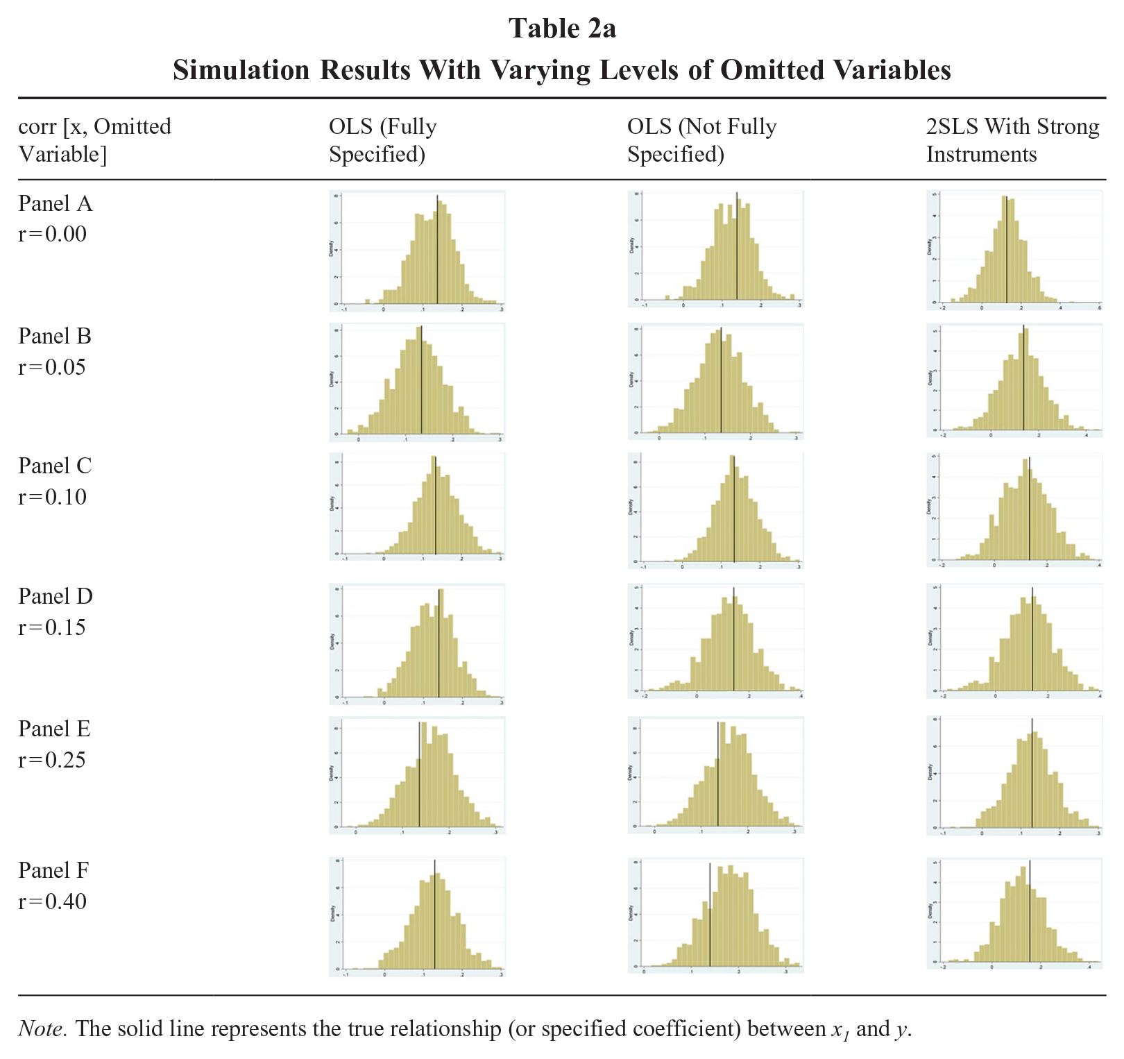
Note. The solid line represents the true relationship (or specified coefficient) between x1 and y.
Simulation Results With Varying Levels of Omitted Variables

Note. The column “SD” reflects the standard deviation of the estimated coefficients across all 1,000 simulations per condition. The percentiles reflect any denoted percentile for the estimated coefficients across those same 1,000 iterations.
Panels B and C in Table 2a and b reflect low levels of correlations with an omitted variable. In each of these panels, we observe that the median coefficients align relatively well with the specified true relationship in virtually all of the models. In fact, the median coefficient from both the fully specified OLS model and the 2SLS estimator are virtually identical. The median coefficient estimated by the not fully specified OLS model is higher than the true relationship, although this deviation is extremely slight (as depicted in Panels B and C and as evidenced by the fact that the differences between coefficients are not statistically significant). At the same time, the distributions of both OLS models are remarkably consistent with one another (the standard deviations are identical), whereas the 2SLS remains wider (the standard deviation is almost twice as large as the OLS models). This is particularly the case as it relates to how often the coefficient is estimated at notably low and high values. We highlight in Panels B and C that the 2SLS estimates coefficients around 0.011 and below approximately 10% of the time and above 0.244 approximately 10% of the time as well. This wide distribution is even more pronounced when the instruments are weakly or moderately related to the independent variable, with the former even estimating a more biased coefficient than the model that is not fully specified. By contrast, both OLS models rarely estimate coefficients this low or high.
Panel D in Table 2 depicts results for our models with a moderate correlation between the focal and omitted variables. In this condition, the non-fully specified OLS model begins to shift slightly to the right, meaning the median coefficient deviates upward marginally from the true relationship. As we depict for this OLS that is not fully specified, the median coefficient is somewhat bimodal, but it is dragged slightly upwards by an uptick in estimates that barely exceed true relationship more than the relatively fewer directly below the true relationship. Again, though, this coefficient is not statistically different from the estimate of the true coefficient. The 2SLS estimates depict an accurate median coefficient, but the distribution is far wider and produces notably low and high estimates more often than the OLS counterparts. This is especially the case when the instruments are weak or moderate, as depicted in Table 2b.
Finally, Panels E and F in Table 2 display results corresponding to relatively high levels of omitted variables. These two conditions feature potential omitted variable bias, which is reflected by the graphics that demonstrate the median coefficient for the not fully specified OLS noticeably exceeds the true relationship. Indeed, the estimate from the not fully specified model is statistically significantly different than the fully specified OLS and the 2SLS model in both of these conditions. Notwithstanding these deviations, however, the distribution of coefficients from the not fully specified OLS model continue to more closely resemble its fully specified counterpart to a much larger degree than does the 2SLS estimator. To this point, the standard deviation of the estimated coefficients from the 2SLS model remains almost twice as large as both OLS models and therefore features a much wider distribution. Interestingly, the 90th percentile of the coefficient for the biased OLS model is approximately the same as the 90th percentile in the 2SLS model (90th percentile = 0.24). Even more, the coefficient from the 2SLS model with less relevant instruments is even more upwardly biased than is the coefficient from the non-fully specified model. This is intriguing because the instruments remain entirely exogenous, therefore demonstrating the detrimental impact of weak instruments.
Discussion of Study 2
Taken together, the results from Study 2 help elucidate the practical relevance of the content analysis we performed in Study 1. As we highlighted in Study 1, our interpretations of the ITCV suggest that most published relationships from management journals do not feature substantive omitted variable bias in terms of causal inference. We reinforced this notion in Study 2. Indeed, the results from our simulations illustrate that omitted variables require relatively high correlations with focal predictors to induce meaningful bias. And even when there is bias in the parameter estimate, the model is still incredibly more efficient than 2SLS with strong instruments, with distributions that closely resemble the perfectly specified model.
Our simulation also illuminates how a potentially biased estimator performs compared to 2SLS with instrumental variables that more closely align with what scholars are often able to locate in practice (i.e., the moderate and weak condition instruments). In fact, one could argue that these instrumental variables are still more appropriate than the types of instruments available in conventional management data since they are perfectly exogenous. This is rarely (if ever) achieved in practice, and scholars suggest that the bias from endogenous instruments is remarkably more pronounced than the bias from weak instruments (Semadeni et al., 2014). Our simulations suggest that the potentially biased model is never significantly biased compared to 2SLS models with moderate or weak instruments but that these two-stage models are dramatically less efficient and induce pervasive Type I and Type II errors relative to the not fully specified OLS technique.
Supplementary Simulation Procedures and Results
In our primary simulation described in the preceding section, we focused primarily on cross-sectional data and estimates derived from OLS and conventional 2SLS models. The reason we incorporated these conditions and corresponding estimators is to minimize the potential biases owing to other elements of the data (Kennedy, 2008). As econometricians routinely describe, limited (i.e., noncontinuous) dependent variables and/or nested (e.g., panel) data can create estimation biases owing to the nature of the types of models necessary to accurately estimate parameters for these types of data (Greene, 2018; Kennedy, 2008; Wooldridge, 2016).
At the same time, we recognize management scholars increasingly require data that do not adhere to the strict assumptions of OLS modeling, especially as it relates to panel data and limited dependent variables (Bowen, 2012; Shook, Ketchen, Cycyota, & Crockett, 2003). In supplementary analyses, then, we restructured our simulation procedure to accommodate these different types of data in order to determine whether omitted variable bias appears differentially pronounced depending on the requisite analytic technique. In each case, we worked to maintain the general properties of our data (e.g., sample size, effect size, variance explained, etc.) while altering only the elements necessary to induce different types of data. Although we do not report the entirety of the results from these supplementary procedures owing to space limitations, we describe each type of supplementary analysis we employed and we summarize the extent to which the results converge with or depart from the primary estimation we describe above.
In one supplementary analysis, we created panel data in order to examine fixed and random effects estimators. We accomplished this by generating observations for 200 “firms” over the course of 5 “years,” such that we maintain a sample size of 1,000. As research on panel data describes, we simulated each observation to feature a panel-level error term and a conventional error term, the latter of which is more similar to the error term in our primary simulation (Certo, Withers, & Semadeni, 2017; Hsiao, 2014). Interestingly, our results from this simulation procedure for both fixed and random effects are almost identical to what we report, except even stronger omitted variables are required to bias the causal inference of the non-fully specified model. This is likely because the within-firm unexplained variance features less potential to confound with the independent and dependent variable owing to the fact that many characteristics of the firm are fixed over time. Nevertheless, our simulation suggests omitted variable bias is even less pronounced with panel data than cross-sectional data. 12
In another set of supplementary analyses, we altered the distribution of the dependent variable and the corresponding estimator required to accommodate any particular distribution appropriate for the ITCV. We respecified our models to feature dependent variables that were truncated at zero (i.e., tobit estimation), count variables that were not overdispersed (i.e., Poisson estimation), count variables that were overdispersed (i.e., negative binomial estimation), and nonnormally distributed (i.e., quantile regression). In all cases, the results were virtually identical to what we report in our primary analyses. This is likely because the nature of correlations between variables—in this case, the correlation between an observed variable and an unobserved confounder—is not particularly sensitive to the distribution of the variable unless the distribution is imposed by transforming the variable (e.g., a ratio) (Certo et al., 2020).
Discussion and Implications
The goal of our research was to examine the extent to which omitted variables appear to bias statistical inference in empirical management research. While management scholarship on omitted variable bias and empirical work that references it have increased over the last couple decades, a growing consensus suggests techniques used to attenuate bias from omitted variables are difficult to implement and can often create more estimation problems than they resolve (Certo et al., 2016; Semadeni et al., 2014). We thus argue it is imperative to better understand the influence of omitted variables in management research. To this end, we first examined empirical relationships published in AMJ, JAP, JOM, and SMJ and analyzed them using the ITCV. We aimed to determine the likelihood that the causal inference of any given relationship was biased from an omitted variable. We consulted the ITCV and applied a variety of stringent interpretations to its value. With these values in mind, we then respecified the simulation Semadeni et al. (2014) employed to better capture the salience of omitted variable bias.
Implications and Contributions
Biased causal inference from omitted variables
One revelation from our study is that not all omitted variables appear to bias statistical or causal inference in meaningful ways. Our analysis of empirical articles published in a variety of top management journals illustrates that the majority of the statistical relationships derived from models not designed to address omitted variables are not apt to feature biased causal inference. To this point, fewer than 5% of published relationships featured biased causal inference if we conceptualize an omitted variable as having the same correlation properties as the average control in a study. Even more, our reasonably conservative interpretation of the ITCV suggests approximately 26% of relationships published in these journals were potentially biased by an omitted variable.
We recognize that we draw conclusions about the prevalence of omitted variable bias in management from published studies, which may result in inaccurate assessments since we do not know the true relationships between variables. This is why some of the scholarship in the area employs simulations that allow scholars to establish relationships between observed and omitted variables (Certo et al., 2016; Semadeni et al., 2014). The results from our simulations suggest that omitted variable bias is not remarkably pronounced except when the omitted variable is highly correlated with structural parameters. As we illustrate in Table 2a and b and describe above, an omitted variable requires a high correlation with independent and dependent variables to produce a distribution of coefficients that deviates noticeably from a fully specified OLS model.
Conceptualizing omitted variables
An important implication from our research involves the nature of omitted variables and what they entail. Stated plainly, our study illustrates that not all omitted variables are created equally and that certainly not all omitted variables invalidate causal inference. Although we agree with the prevailing notion in the literature that most relationships management scholars study feature omitted variables (Hamilton & Nickerson, 2003), our findings suggest that not all of these omitted variables are problematic. In fact, our content analysis reveals that omitted variables would need correlations with structural variables at levels higher than most focal constructs in management research to bias causal inference. Even more, the ITCV value reflects partial correlations, whereas management scholars almost always report zero-order correlations that are higher than their partial counterparts.
Our study therefore highlights three important dimensions scholars should consider concerning omitted variables. First, it is imperative to consider what potential omitted variables might exist that exhibit strong enough relationships to induce empirical bias. As we contend in this study, the ITCV provides a tangible benchmark that scholars can use to determine a threshold magnitude. But it is incumbent on researchers themselves to think theoretically about what variables could even possess the requisite correlations. Second, researchers can consult control variables and think extensively about whether they are analogous to potential confounding factors, weaker than a conceptualized omitted variable, or stronger than a variable that may be omitted from the model. We provided several potential interpretations scholars can use for incorporating controls as proxies for omitted variables. Finally, it is paramount to think more extensively about the directionality of the correlations with omitted variables and how that may influence results. This is an important implication because only one study to our knowledge has described how the correlation with omitted variables can suppress or enhance estimated relationships (Certo et al., 2016).
Empirical estimators and model selection for macro and micro research
Another important implication from our research involves the veracity of “biased” OLS models relative to their instrumental two-stage counterparts. As we highlighted throughout this study, scholarship on omitted variable bias often promotes two-stage instrumental variable techniques as the premier solution for attenuating bias from endogeneity (Bascle, 2008; Kennedy, 2008; Stock et al., 2002; Wooldridge, 2010). At the same time, this research continues to highlight that such models can be problematic because they are inefficient and can produce more bias than OLS unless they adhere to strict and often unattainable standards (Certo et al., 2016; Larcker & Rusticus, 2010; Semadeni et al., 2014). Econometricians have therefore cautioned against defaulting to two-stage instrumental techniques unless absolutely necessary (Kennedy, 2008).
Our results in Table 2a and b corroborate these potential problems with instrumental variable modeling. As we illustrate with the distributions of coefficients across our simulations and show with descriptive statistics, the 2SLS technique is indeed remarkably less efficient than the fully specified or not fully specified OLS counterparts. In other words, the 2SLS model is more likely to predict coefficients at more extreme ends of the high and low tail than either OLS model (including the model with potential omitted variable bias). We uncovered these distributions even in our simulation with strong instruments that are completely exogenous. In our 2SLS models with weak and moderate instruments that are still entirely exogenous, we find that the 2SLS model can estimate more biased coefficients than a not fully specified OLS model as strength of the omitted variable increases.
The results from our simulations raise questions as to whether two-stage instrumental variable techniques are more consistent than potentially biased OLS (or other types of models that we describe in our supplementary analyses) except in the most pressing circumstances and when the instruments are incredibly relevant and exogenous. In practice, and given the correlations with control variables we observed in our content analysis, it is unlikely scholars will uncover instruments with such desirable characteristics. Scholarship in the econometrics literature has noted these issues with conventional instruments, and it has therefore begun to introduce alternative approaches to integrating tenable instrumental variables. For instance, Baum and Lewbel (2019) describe an increasingly pervasive technique that transforms heteroskedastic errors into appropriate instruments, and Le Gallo and Páez (2013) develop an approach that simulates instrumental variables that contain desirable properties. Although it is well beyond the scope of our present research to explicate these procedures, they demonstrate the types of alternative estimation approaches econometricians are developing.
It is important to note that these procedures rely on the mathematical properties of instruments rather than theoretical justifications. For decades, econometricians have argued that instrumental variable modeling is a mathematical exercise but that theory can help inform the underlying data generation practices. In management research, though, scholars often misinterpret this to mean that instruments must have theoretical justifications for their inclusion. Theoretically justifying heteroskedastic or synthetic instruments is implausible, which is consistent with the idea that the underlying mathematics are agnostic to any theory.
Notwithstanding this discussion, for a variety of reasons, we are hesitant to suggest scholars move away entirely from conventional two-stage instrumental techniques. First, although the distribution of the coefficients in the 2SLS model is wider and the variance is higher than OLS, the median coefficient produced in our simulations from 2SLS was not biased except when the instruments were weakly correlated with the independent variable. Second, two-stage modeling is the gold standard for addressing omitted variable bias (Kennedy, 2008; Wooldridge, 2010). In the presence of desirable instruments, two-stage techniques at the very worst provide researchers more information to determine whether there is potential omitted variable bias. Finally, two-stage estimation continues to get more efficient and less computationally costly.
We recognize that more micro-oriented scholarship rarely (if ever) encounters these issues with two-stage modeling and instrumental variables because these types of estimation procedures have not yet been widely adopted in organizational behavior research. At the same time, the potential for omitted variable bias is still a critical concern for micro-related empirical research (Meade, Behrend, & Lance, 2009). As such, we caution against ignoring the benefits of the ITCV simply because its benefits for two-stage instrumental variable modeling seem irrelevant for this particular research domain. Instead, we contend that the ITCV proves incredibly beneficial for this literature because it may provide some insight as to the nature of potential bias from an omitted variable that would otherwise involve speculation and considerable guesswork. Even more, it may allow organizational behavior scholars to avoid instrumental variable modeling, which would likely prove challenging to incorporate given the relative absence of unused variables that could be applied as instruments (Atinc et al., 2012). In sum, even though micro-oriented scholarship often does not address omitted variable bias via estimation procedures, the ITCV offers a mathematical tool for this research to empirically examine the veracity of parameter estimates, causal inference, and corresponding effect sizes.
Using the ITCV in empirical research
One particularly intuitive approach scholars can use to incorporate the ITCV in their studies to consider issues related to omitted variables and two-stage modeling is to simply consult the ITCV value after employing an estimator that does not explicitly account for omitted variable bias. If the ITCV is sufficiently high, scholars can likely proceed without much concern for omitted variable bias. If the ITCV is not sufficiently high, we encourage scholars to then utilize two-stage modeling and appropriate instruments (see the decision tree in Figure 3). Naturally, scholars should still consider other sources of endogeneity (e.g., measurement error and reverse causality).
We must reiterate here that the ITCV only addresses causal inference and does not consider biased parameter estimates owing to an omitted variable. There is likely a range over which a given estimate may produce a nonzero coefficient, although the practical interpretation of that coefficient may change dramatically depending on the influence of an omitted variable. In fact, and as we describe in the appendix, the RIR can provide some insight as to what this range may entail. We therefore caution scholars against making definitive statements that suggest their models are entirely unbiased from omitted variables because of an adequately high ITCV value. Instead, we encourage scholars to follow extant work in the area and focus the ITCV only on causal inference and general empirical support for a hypothesis.
Conclusion
Omitted variables are inherent in management scholarship, but our research demonstrates that their presence is not always associated with biased causal inference. Indeed, not all omitted variables create substantive bias, and oftentimes the proposed estimation remedy is more detrimental than the bias from confounders themselves. Our goal in this study was to help scholars use the ITCV technique to think more exhaustively about the nature of omitted variables in empirical analyses, especially as it relates to two-stage instrumental variables techniques.
Footnotes
Appendix 1
Appendix 2
Acknowledgements
We gratefully acknowledge Trevis Certo, Matt Semadeni, and the participants in the Research Methods Division session of the Academy of Management 2019 conference for their helpful comments on earlier versions of this manuscript. We also thank Associate Editor Aaron Hill and two anonymous reviewers for their invaluable insights and contributions to our research. We further appreciate Wookyung Lee for all of his help collecting data for this study.