Bells in Space

Abstract

Social and interregional inequality patterns across US states from 1929–2012 are analyzed using exploratory space–time methods. The results suggest complex spatial dynamics for both inequality series that were not captured by the stylized model of Alonso. Interpersonal income inequalities of states displayed a U-shaped pattern ending the period at levels that exceeded the alarmingly high patterns that existed in the 1920s. Social inequality is characterized by greater mobility than that found for state per capita incomes. Spatial dependence is also distinct between the two series, with per capita incomes exhibiting strong global spatial autocorrelation, while state interpersonal income inequality does not. Local hot and cold spots are found for the per capita income series, while local spatial outliers are found for state interpersonal inequality. Mobility in both inequality series is found to be influenced by the local spatial context of a state.

Keywords

urban and regional economic development economic growth and development policy and applications poverty income distribution income inequality social and political issues growth development and convergence urban and regional spatial structure spatial structure time series and forecasting models economic analysis methods spatial statistics and spatial econometrics spatial analysis

Introduction

Through a synthesis of previous research on regional economic development, Alonso (1980) provided a stylized model of how to explore the relationships between the dynamics of five different aspects of economic development: (1) economic growth, (2) social inequality, (3) regional inequality, (4) geographical concentration of population, and (5) demographic transition. The bell analogy relates to the so-called inverted U pattern, posited by Kuznets (1955) for social or personal income, inequality, and Williamson (1965) for regional inequality, in that the shape of the bell portrays the expected evolution of each type of inequality as an economic system develops. Alonso also suggested the bell-shaped curve gave good approximation to the evolution of the three other phenomena.

While immensely important for regional scientists, these bells leave the geographic dimensions of these dynamics largely untouched. These trajectories do tell us something about the dynamics of some overall, whole map, statistic, but they are silent on the spatial footprint of those dynamics. Although Alonso also argued that two of these phenomena—regional inequality and geographical concentration—were spatial in nature his definition of spatial is a limited one in that for both attributes the concentration, or inequality, is actually a summary measure of the values of those attributes and is invariant to the spatial distribution of the underlying phenomena across the units (i.e., states, counties, and regions).

In this article, I revisit two of these five bells to consider the spatial dynamics of regional income inequality and interpersonal income inequality. Drawing on recently developed methods of exploratory space–time data analysis, I first examine each series individually followed by a comparative analysis. Specific attention is given to the rate of mobility, or spatial change, in the inequality measure over time. Discrete Markov chains (DMCs) and their spatial extensions are applied to series for the US states over the period 1929–2012.

The remainder of the article is organized as follows. I first discuss the motivation for focusing on a joint treatment of regional and interpersonal income inequality in the second section. This is followed by a description of the data series and particular spatial analytics of the research design in the third section. In the fourth section, the results of the analysis are examined and the article concludes with an overview of the key findings and directions for future research.

Interpersonal and Interregional Income Inequality

This article focuses on, and contrasts, patterns of two types of inequality, interpersonal and interregional, or what Alonso referred to as social and regional inequality, respectively. Both types of inequality have attracted enormous attention in large literatures.¹ However, these two literatures are largely independent. Alonso’s reasoning some thirty-five years ago suggested that the two inequality series should be tied together. One of the main goals of this article is to reconsider the two forms of inequality in tandem using the US experience as the empirical setting.

Interpersonal Inequality

In the United States, the 1970s marked the end of a long period of declining income inequality that began during the 1940s. Initially the reversal was gradual, but beginning in the 1980s the increase in inequality accelerated. The nature of this shift has been rather dramatic and, unsurprisingly, has attracted much attention from both academics and policy makers (Galbraith 2012; Noah 2012; Stiglitz 2012; Wilkinson and Pickett 2006). Piketty and Saez (2013) note that one consequence of this rise in interpersonal US income inequality has been that the share of income going to individuals in the top percentile of the income distribution has more than doubled from just under 10 percent in the 1970s to over 20 percent in 2010. At the same time, more than 15 percent of US national income has shifted from individuals in the bottom 90 percent to those in the top decile of the distribution. The shift itself has also been particularly concentrated within the top decile, as more than 60 percent of US aggregate income growth between 1976 and 2007 has been absorbed by the top 1 percent of the distribution (Piketty and Saez 2013, 458).

The use of metaphors to describe temporal patterns of aggregate interpersonal inequality continues in the modern literature as reflected in the arguments of Piketty and Saez (2006, 201) who note that:

The overall pattern of the top decile share of the century is U-shaped.

Of course, they go on to note that this is not an inverted U, and thus their finding is at odds with the stylized arguments of Kuznets (1955), and, I would add, Alonso.

A number of arguments have been put forth regarding the forces behind these personal income inequality dynamics in the United States. Increasing international trade in the form of import competition over the past several decades has been linked to inequality, yet the estimates of trade’s contribution to rising inequality has varied from highs of 50 percent (Wood 1994) to lower shares of 20 (Leamer 1994) to 10 percent (Krugman and Lawrence 1993), with some studies finding no significant linkage between trade and inequality (Sachs et al. 1994). However, results in Rigby and Breau (2008) challenge the findings that trade has little impact on rising inequality, as their examination of the relationship at a finer subnational spatial scale revealed a positive association between the growth of trade and wage inequality.

The impact of skill-biased technical change (SBTC) has been argued by some to be a significant factor being rising inequality. By increasing the demand for more highly educated labor, SBTC is said to put upward pressure on their wages and, conversely, downward pressure on the wages of less educated workers leading to a widening of wage inequality. The estimates of SBTC’s contribution to rising inequality are on the order of 25–40 percent (Breau 2007). In contrast, Card and DiNardo (2002) suggest that SBTC is not a significant source of wage inequality increases in the United States.²

In addition to trade and technological changes, a number of institutional sources of raising US income inequality have been put forth. Changes in the US tax system through the 1981 Economic Recovery and Taxation Act and the Tax Reform Act of 1986 have resulted in increased regressivity of personal income taxes (Levy and Murnane 1992, 1346). Similarly, corporate income taxes have declined from a high of 39.8 percent in the 1940s to 9.9 percent in 2012 (Stiglitz 2014, 9) the benefits of which have disproportionately accrued to high-income individuals.

Alongside changes in tax policies, Kristal (2013) argues that the decline in unionization, from a high of 24 percent in 1945 to under 8 percent by 2012, caused a decline in labor’s share of national income resulting in increased inequality. Gordon (2014) estimates that declining unionization accounted for about a third of the increase in inequality in the 1980s and 1990s. Card and DiNardo (2002) point to a fall in the real value of the minimum wage in the United States over the 1970–2000 period as explaining some 90 percent of the variation in the gap between the 90 percent and 10 percent wage percentiles.

These arguments concern the evolution of aggregate interpersonal inequality at the national level. There has been a smaller related research thread examining patterns at the subnational scale.³ A number of studies have focused on the variation in interpersonal income inequality across regional economies in the United States (Levernier, Rickman, and Partridge 1995; Partridge 1997; Partridge et al. 1998; Panizza 2002; Partridge 2005; Frank 2009). Changes in inequality at the subnational level have been associated with changes in demographic variables, such as immigration (Chakravorty 1996; Nielsen and Alderson 1997), household, and gender composition (Madden 2000; Essletzbichler 2015), as well as industrial economic restructuring (Odland and Ellis 2001), labor sorting (Moretti 2013; Andersson, Klaesson, and Larsson 2014), and exposure to international trade (Rodríguez-Pose 2012).

Many times, the question of interest is the impact of interpersonal inequality on the region’s rate of economic growth. To the extent that inequality may have a negative impact on economic growth, spatial variations in interpersonal inequality may result in an uneven regional growth. The evidence on this relationship is mixed across studies. Partridge (1997) finds a positive relationship between different measures of inequality and US state income growth. Using a different methodological framework, but similar data, Panizza (2002) finds no evidence of a positive relationship between changes in inequality and changes in growth. While these two studies employed data at ten-year intervals, Frank (2009) develops an annual series of state income inequality and finds a positive relationship between the top decile share of income in a state and the state’s economic growth. Additionally, the trends in inequality at the state level are found to mimic the overall trend in aggregate US inequality.

Interregional Inequality

The second of Alonso’s five bells examined here concerns regional inequality. While interpersonal inequality focuses on the inequalities between individuals, interregional inequality is concerned with the inequalities between the average incomes of regions within a national system. Relative to the number of studies of regional interpersonal income inequality reviewed above, the literature on interregional income equality is considerably larger, dating back to early work by Myrdal (1957); Easterlin (1960); Williamson (1965). This early work focused on the general empirical regularity that the level of inequality between regions in a national economy tended to display an inverted-U pattern, increasing during early stages of national development but then declining as the economy reached high levels of development.

Since this early work, the number of studies of regional interregional inequality has exploded and an overview of this work is beyond the current scope.⁴ Broadly speaking, studies of interregional inequality can be placed into two groups based on the methodological approach adopted, those focusing on decompositions of regional inequality and those adopting a more confirmatory approach that subsumes interregional inequality within the question of regional income convergence.

The decomposition studies typically define a mutually exclusive and exhaustive partitioning of the individual economies into regions and then use this regionalization to separate total inequality into two components: interregional inequality and intraregional inequality. The former reflects the inequality due to the differences in the average group mean incomes, while the latter measures inequality between economies assigned to the same region. Work on the United States has demonstrated that within-region inequality tends to be the larger of the two inequality components (Krugman 1991; Fan and Casetti 1994; Rey 2004). This echoes similar findings from studies of other national systems (Shorrocks and Wan 2005).

A slightly different perspective on interregional inequality can be seen in the work using finer spatial scales to measure inequality and relating that to growth at the more aggregate level (Amos Jr., 1983, 1988; Janikas and Rey 2005, 2008). For example, rather than measure interpersonal income inequality, interregional inequality between counties is used. Both sets of studies report a great deal of heterogeneity in the inequality–growth nexus across the states. Moreover, Janikas and Rey (2005) find that a very strong positive relationship between spatial clustering in state income levels and national economic growth in income takes on a different form at a lower spatial scale where a generally negative relationship holds between intrastate spatial clustering and state-level income growth.

The second group of studies on interregional inequality is the vast literature on the so-called regional economic convergence (Rey and Le Gallo 2009). Alternative types of convergence have been examined in the literature, with the most focus being on σ- and β convergence. σ convergence refers to a decline in the dispersion in the cross-sectional distribution of regional incomes over time. β convergence is tied to neoclassical growth models suggesting that the growth rate in a region’s income is a positive function of the distance from its steady state. Empirical analysis of β convergence typically specifies income growth rates as a function of initial incomes and variables that condition for the steady state of each region.

For the United States, a number of studies have found general long-run evidence for both σ (Rey and Dev 2006; Young, Higgins, and Levy 2008) and β convergence (Barro and Sala-i Martin 1991; Bernard and Jones 1996; Rey and Montouri 1999). However, some question if these long-run trends are now being reversed (Ganong and Shoag 2015). Moreover, both σ and β convergence have been subjected to much criticism in the regional science literature for their neglect of spatial dependence and spatial heterogeneity—characteristics of spatially referenced data that tend to be the norm rather than the exception. These forms of convergence also provide only summary views of the distribution of regional incomes and are generally silent on the internal dynamics of the distribution (Rey and Le Gallo 2009). These criticisms have led to a related literature in spatial distribution dynamics where a new set of exploratory methods have been suggested to study the full distribution of regional incomes and the role of spatial effects in their evolution (Rey 2014).

Interpersonal and Interregional Inequality—Separated at Birth?

While the literatures on social and regional inequality have matured since Alonso’s article, they have done so as largely separate endeavors with only limited cross fertilization. Indeed, as Metwally and Jensen (1973) note, measures of interregional inequality fail to take into account interpersonal income inequality either nationally or within regions. By the same token, focusing on the aggregate national personal income distribution masks the geographical dimensions of inequality dynamics.

There are good reasons for considering personal and regional income inequality jointly. The work on interpersonal income inequality has used measures of inequality defined on personal income distributions for each state and then focused on examining the determinants of these derived measures. By contrast, the interregional inequality literature has used an average income measure (typically per capita) for each region and explored the distribution of these averages over space and time.

Consequently, the two literatures are studying different moments of the same distribution. More specifically, let y_j _,r,t represent the income of individual j in region r in period t. The interpersonal inequality literature has focused on measures related to the dispersion in the distribution of f(y_i _,r,t) within a particular region:

σ {(y)}_{r, t}^{2} = \frac{1}{N_{r, t}} \sum_{j \in r} {(y_{j, r, t} - {\bar{y}}_{r, t})}^{2},

where ${\bar{y}}_{r, t} = \frac{1}{N_{r, t}} \sum_{j \in r} y_{j, r, t}$ and N_r , _t is the population of r in time t. Analysis of interpersonal inequality⁵ has focused on the distribution of $σ {(y)}_{r, t}^{2}$ over r = 1,2, …, R regions and t = 1,2, …,T time periods, while the regional inequality has examined the distribution of ${\bar{y}}_{r, t}$ over the same regions and time periods.

In addition to the linkage between the distribution that ties the two literatures together, the second reason to consider both interpersonal and regional inequality dynamics is that there could be gains achieved from exploiting the complementary nature of the methodologies employed in the two literatures. In the interpersonal inequality literature, the focus has largely been on confirmatory modeling of the determinants of inequality or the relationship between inequality and growth. Conversely, in the regional inequality work, the emphasis has been on the underlying spatial patterns of the level of incomes and the dynamics of those patterns. As the latter is more exploratory in nature, while the former is confirmatory it seems prudent to adopt the exploratory approach to the case of interpersonal inequality. Essentially, the interpersonal inequality literature has simply skipped over the exploratory phase, and in this article I revisit this issue.

A third justification for focusing on both regional interpersonal and interregional inequality is that together the two components represent a decomposition of total national interpersonal income inequality (Rietveld 1991). This follows from the definition of the terms in (1), which can be extended to measure the total inequality (variation) in the national system:

σ {(y)}_{t}^{2} = \frac{1}{N_{t}} \sum_{j} {(y_{j, t} - {\bar{y}}_{t})}^{2},

where ${\bar{y}}_{t}$ is the national mean of incomes in period t. The variance of national personal incomes can then be decomposed into interregional and aggregate intraregional components:

σ {(y)}_{t}^{2} = σ {(y)}_{INTER, t}^{2} + σ {(y)}_{INTRA, t}^{2} .

with

σ {(y)}_{INTER, t}^{2} = \frac{1}{N_{t}} \sum_{r} N_{r, t} {({\bar{y}}_{r, t} - {\bar{y}}_{t})}^{2}

and

σ {(y)}_{INTRA, t}^{2} = \frac{1}{N_{t}} \sum_{r} \sum_{j \in r} {(y_{j, r, t} - {\bar{y}}_{r, t})}^{2} .

The recent focus on inequality in the United States has been concerned with (2). On the one hand, this has, to date, ignored the underlying components in (4) and (5). Alonso’s two bells, on the other hand, do not consider the decomposition between interregional and intraregional inequality explicitly. Rather, his definition of interpersonal income inequality is (2), while by interregional inequality Alonso pointed to (4). Aggregate intraregional variance is ignored in his five-bell system but could be viewed as a derived decomposition:

σ {(y)}_{INTRA, t}^{2} = σ {(y)}_{t}^{2} - σ {(y)}_{INTER, t}^{2} .

In what follows, I explicitly consider both interregional and aggregate intraregional variance together.

Bells in Space

The bell analogy, while a powerful metaphor to help frame our thinking about inequality dynamics, also brings to the fore an important issue regarding distributions. More specifically, one is often naturally drawn to think of a bell as a stylized representation of a Gaussian distribution, and in the case of questions about income inequality distributions are a central concern. However, in the regional context, there are two problems with this tendency. The first is that the bell as distribution metaphor is different from what Alonso suggested as his view was that the bell traced out the path of a scalar summary measure of some distribution over time. For per capita income, that summary measure is the mean of the distribution for a set of regions, with the distribution being measured at each point in time. For personal income inequality the summary measure is something like a Gini coefficient and the bell traces its evolution over time, but again the statistic is derived from distributions of incomes measured at different points in time.

The second issue with the bell analogy is that the distributions under consideration are explicitly univariate distributions. Without this, the scalar summary measures of those distributions lose their conceptual underpinnings. This perspective comes at a cost however, as univariate distributions do not afford a consideration of spatial dependence or spatial heterogeneity. Spatial dependence becomes relevant whenever there is potential for the regions to interact, which would be reflected in migration, capital flows, trade, and other phenomena that tie regions together.

Spatial heterogeneity would be reflected in situations where different subsets of the regions in the system display different types of behaviors, such as in the case of convergence clubs (Chatterji and Dewhurst 1996) or poverty traps (Bowles, Durlauf, and Hoff 2008), which may be driven by variations in economic structure (i.e., industry mix and demographic composition), across regional economies. The presence of either spatial dependence or spatial heterogeneity requires a shift in thinking from a univariate to a multivariate perspective since the latter affords the formal representation of these spatial effects.

Here we see another asymmetry in the two inequality literatures. The regional convergence literature has embraced the spatial dimensions in empirical and, to a lesser extent, theoretical, work. By contrast, the work on intraregional interpersonal income inequality has treated the observations from each of the regions as independent from those in other regions. The determinants of interpersonal income inequality within a state have been viewed as originating within that state–spatial interactions have been largely ignored. Given that there is growing evidence that the adoption of spatial methods, be they spatial econometrics or exploratory spatial data analysis, has provided important insights into the regional convergence literature, it seems worthwhile to extend these methods to the spatial dynamics of interpersonal regional income inequality as well.

Methods

The joint consideration of interpersonal regional income inequality and interregional income inequality requires the development of times series of observations on both types of inequality for each region within a national system. The two series are then analyzed via the same set of space–time analytics.

Data

The data used to measure state-level interpersonal income inequality comes from a unique series constructed by Frank (2009). It is based on pretax-adjusted gross income reported by the US Internal Revenue Service which includes wages and salaries, capital income, and entrepreneurial income. The particular series examined in this article are the income shares of the top percentile (S01) and top decile (S10) of the population annually for the period 1916–2012.

In addition to the income shares, data on per capita income for the states are obtained from the US Department of Commerce, Bureau of Economic Analysis⁶ covering the period 1929–2012. State per capita incomes (SPI) are normalized relative to the national mean (USPI) for each year in the sample: $RSP I_{r, t} = \frac{{SPI}_{r, t}}{{USPI}_{t}}$ .⁷

Methods: Distributional Dynamics

The central focus in this article is an examination of the distributional dynamics of interpersonal and regional income inequality in the United States over the period. More specifically, the internal distributional dynamics which reflect the extent of mobility of the states within the respective distributions over time are a key concern. Both the summary measures of mobility and the role of spatial structure and interactions are considered.

Discrete Markov chains

The departure point for investigating inequality dynamics is the estimation of DMC. These are formed for regional series at two points in time: $y_{t} \in [0, \infty)$ and $y_{t + d} \in [0, \infty)$ with cummulative distribution function F(y_t , y_t _+d). The DMC maps F (y_t , y_t _+d) into a k × k transition matrix, where k is the number of discrete space states the chain can be in at any moment in time. The states of the chain are defined as: $0 \leq c_{1, t} \leq c_{2, t} \leq \dots \leq c_{k, t}$ . The transition probability matrix for the DMC takes the following form:

p_{i, j} = \frac{Pr (c_{i - 1, t} < y_{r, t} \leq c_{i, t} \cap c_{j - 1, t + d} < y_{r, t + d} \leq c_{j, t + d})}{Pr (c_{i - 1, t} < y_{r, t} \leq c_{i, t})},

where y_r _,t is the observed value of the series for region r in period t. Thus, (7) gives the conditional probability that a region r in class i in period t moves into class j in period t + d.⁸

One assumption generally made in the literature is that these probabilities hold for all R regions and time periods. This allows for the estimation of P using paired samples of $(y_{r, t}, y_{r, t + d}) \forall r = 1, 2, \dots, R$ drawn from F (y _t, y _t+d) using maximum likelihood:

{\hat{p}}_{i, j} = \frac{\sum_{r = 1}^{R} I (c_{i - 1, t} < y_{r, t} \leq c_{i, t} \cap c_{j - 1, t + d} < y_{r, t + d} \leq c_{j, t + d})}{\sum_{r = 1}^{R} I (c_{i - 1, t} < y_{r, t} \leq c_{i, t})},

and

{\hat{π}}_{i, t} = \frac{1}{n} \sum_{r = 1}^{R} I (c_{i - 1, t} < y_{r, t} \leq c_{i, t}),

where $I (.)$ is an indicator function with value 1 if the condition is true and 0 otherwise, and ${\hat{π}}_{i, t}$ is the marginal probability of a region being in discrete state i of the distribution in time t.⁹

The DMC framework can be used to examine a number of dimensions of regional inequality distribution dynamics. These include different measures of the mobility in the distribution reflecting specific types of movement within the distribution. Additionally, comparison of the dynamics across regional inequality series or at different points in time allows for an examination of alternative forms of heterogeneity in the dynamics.

The question of whether the series can be viewed as a single Markov chain or M separate chains is addressed through a test of homogeneity of the Markov transition probability matrices. Following Bickenbach and Bode (2003), I adopt two formal tests of homogeneity:

Q^{(M)} = \sum_{m = 1}^{M} \sum_{i = 1}^{n} \sum_{j \in A_{i}} n_{i | m} \frac{{({\hat{p}}_{i, j | m} - {\hat{p}}_{i, j})}^{2}}{{\hat{p}}_{i, j}},

H_{o} : p_{i, j | m} = p_{i, j} \forall m = 1, 2, \dots, M,

Q^{(M)} \sim χ^{2} (\sum_{i = 1}^{N} (a_{i} - 1) (b_{i} - 1)),

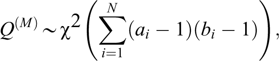
where a_i is the number of elements in A_i which is the set of nonzero transition probabilities in the ith row of the transition matrix estimated from the entire sample, and b_i is the number of the regimes for which a positive number of observations is available for the ith row $(B_{i} = {m : n_{i | m} > 0})$ .

The likelihood ratio test for the same null takes the following form:

L R^{(M)} = 2 \sum_{m = 1}^{M} \sum_{i = 1}^{n} \sum_{j \in A_{i | j}} n_{i, j | m} l n \frac{{\hat{p}}_{i, j | m}}{{\hat{p}}_{i, j}},

where $A_{i | m} = {j : {\hat{p}}_{i, j | m} > 0}$ is the set of nonzero transition probabilities in the ith row of the transition matrix estimated from the mth regime. LR ^(M) has the same asymptotic distribution as Q ^(M).

The homogeneity testing framework is quite general and permits the examination of a number of interesting special cases reflecting alternative definitions of the regimes. For example, if different variables can be used to measure inequality, a test of the similarity of the dynamics of the inequality reflected in the two series can be considered using this framework. In the current context, we can compare intraregional interpersonal inequality and its dynamics over space to that of interregional income inequality dynamics.

Spatial autocorrelation

To complement the focus on distributional dynamics, a spatial perspective is also adopted to explore the nature and extent of any spatial clustering in the two inequality series. For each year and series, both global measures of spatial autocorrelation and local indicators of spatial association are calculated. The global measure is Moran’s I:

I_{t} = \frac{n}{S_{0}} \frac{\sum_{r} \sum_{s} z_{r, t} w_{r, s} z_{s, t}}{\sum_{r} z_{r, t}^{2}},

where w_ij is the value from a row-standardized, queen-based contiguity matrix for the forty-eight conterminous US states, S ₀ is the sum of all the elements in W, and $z_{r, t} = y_{r, t} - {\bar{y}}_{t}$ . The global measure at time t can be used to test if the inequality series departs from a random spatial process.

The local indicators of spatial association are:

I_{r, t} = \frac{n}{S_{0}} \frac{\sum_{s} z_{r, t} w_{r, s} z_{s, t}}{\sum_{r} z_{r, t}^{2}},

which provide for an exploration of localized spatial clustering which might be driving the global pattern from (12) or departing from the global process (Anselin 1995).

Space–time measures

To examine the role of space in shaping the distributional dynamics, a number of spatial extensions to the DMC are also employed. The spatial Markov chain (Rey 2001) conditions the transition probabilities facing a regional series on its regional context. This is a specific form of the general homogeneity framework above, where the regimes are defined based on the spatial lag of the inequality series. More specifically, the spatial lag is defined as $L_{r, t} = \sum_{s} w_{r, s} y_{s, t}$ and is itself discretized into quintiles. A formal test of whether the transitional dynamics are homogeneous across the regimes based on the spatial lag quintiles is then carried out.

Results

Dynamics of Inequality

Figure 1 contains the time series for the mean income shares claimed by the richest 0.10 (S10) and 0.01 (S01) of individuals, with the means taken over the states. The two shares move in concert and reflect the general U pattern reported by Piketty and Saez (2006) where high levels of inequality mark the beginning of the sample followed by a long period of declining inequality from the early peak in 1930 through 1980. This decline sharply reversed in the 1980’s returning levels of inequality to their historical highs.

Figure 1.

Mean 0.10 and 0.01 income shares for states, 1916–2012.

Figure 2 reports the maximum of the income shares for S01 and S10. In the most extreme case, Florida’s 0.10 income share reached almost 0.80 of total personal income in 1929, with its 0.01 share claiming an astounding 0.60 of total personal income for the state. While the maximum shares display the initial decline from the peaks that were seen in the average shares, the growth in the maximum shares after 1980 is not as pronounced as the increase in the mean inequality seen in Figure 1.

Figure 2.

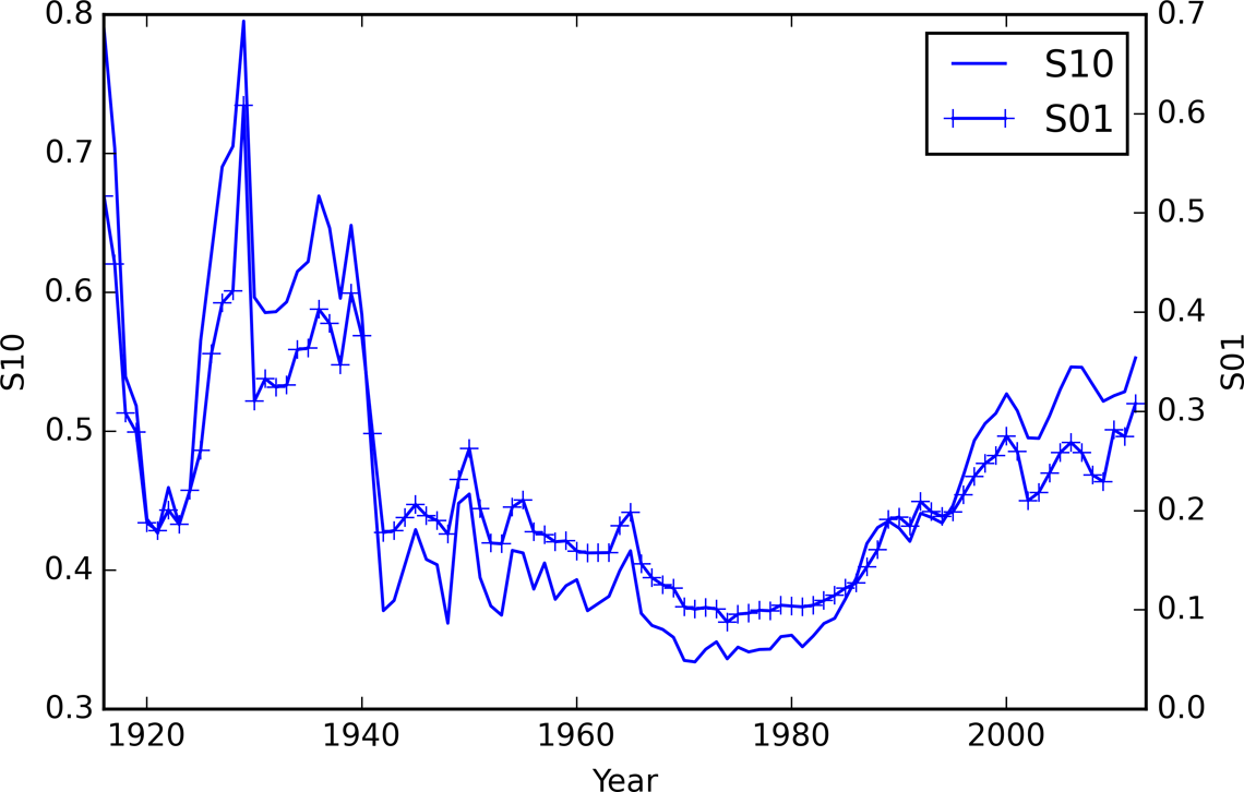
Maximum 0.10 and 0.01 income shares for states, 1916–2012.

Figure 3 displays the evolution of the global quintile distribution over time.¹⁰ The number of states with 0.01 income shares falling into each quintile fluctuates in interesting patterns. Generally speaking, three different epochs where the quintile distribution takes on different forms can be identified. In the early part of the sample up to 1940, the upper quintiles dominate reflecting a period of high personal income inequality. In the second epoch, 1940–1980, the first and second quintiles grow in importance at the expense of the fifth quintile, which starting in 1966 up until 1988 contained no states. The final epoch starts in 1988 with the resurgence of the fifth quintile and its clear dominance. Indeed, for the years 2004–2008 all states have 0.01 shares in the fifth global quintile.

Figure 3.

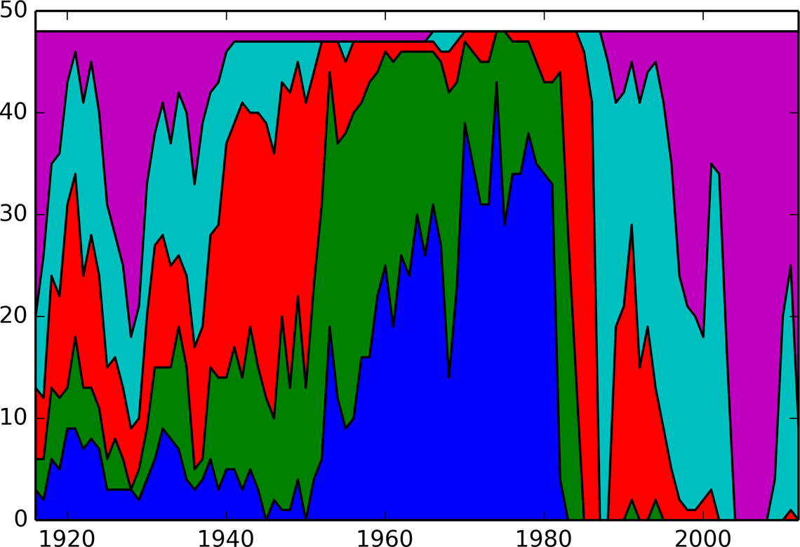
Global quintile distribution, 0.01 income shares for states, 1916–2012.

If the income share quintile distribution is compared to the global quintile distribution for relative per capita income of the states in Figure 4 clear distinctions between these two series emerge. For relative incomes, there is a general pattern of convergence as the first and fifth quintiles begin the sample period as dominant but loose states over time. The internal quintiles (Q2, Q3, and Q4) gain states together throughout most of the period with a shift toward the end of the sample where the middle quintile begins to shrink, while the second and fourth continue to expand. There is also a renewal of growth for the first and fifth quintile toward the very end of the sample. Unlike the case for the income share quintile distribution, there are no clear epochs in the evolution of the per capita income quintile distribution. Moreover, the each of the five quintiles in the share distribution experiences periods where there are no states falling in that quintile, while for the per capita quintile distribution none of the global quintiles is ever empty.

Figure 4.

Global quintile distribution, per capita income for states, 1929–2012.

Spatial Distribution of Inequality

Figure 5 displays the global quintile maps for the 0.01 share of incomes for the forty-eight lower US states in the selected years. Since they are derived from a pooling of all annual series, the quintiles are fixed for each of the maps in order to more readily visualize the evolution of the spatial patterns. Examination of the global quintiles reveals that the maximum share of the top 0.01 of households was 0.608 over the sample period with a minimum of 0.062. To enter the fifth quintile required that the 0.01 share exceed 0.151 in a given year. The evolution of the map patterns reveals the spatial footprint of the summary inequality dynamics behind Figures 1 –3.

Figure 5.

Top 0.01 income share by global quintiles selected years. Legend values are upper bound of each quintile.

While the general U pattern of interpersonal income inequality in the United States has been much commented upon, the spatial distribution of inequality and the evolution of these patterns suggests that even when the overall level of inequality are roughly equal, as in the first and third epochs in the time series in Figure 1, the spatial distribution associated with these high-inequality periods can be distinct. In the modern high-inequality era, the spatial homogenization of inequality is much stronger than in the earlier high-inequality era of the 1920s. In the third epoch, the increase in inequality was associated with a rapid change in its spatial distribution between 1988, where states are in either the first or second quintiles, and 1997 where all states move to the fourth or fifth quintiles. As was seen in the time series plots of the summary income shares, this period reflected rapid increase in inequality and this is clearly reflected in its spatial distribution, as by 2005 each state’s 0.10 income share is in the upper quintile. By contrast, the spatial patterns of inequality in the 1920 period are much more heterogeneous.

The time series of maps for state relative per capita incomes by global quintile for the same select years are shown in Figure 6. In contrast to the maps of 0.01 income shares, the state per capita income maps display considerably less differentiation across the three epochs. The general trend is a reduction in dispersion in relative per capita incomes reflected in states moving out of the first and fifth quintiles over time, as was suggested by Figure 4. However, there is a clear spatial signature to these changes as the cluster of low-income southeastern states in the early epoch breaks apart beginning with the second epoch.

Figure 6.

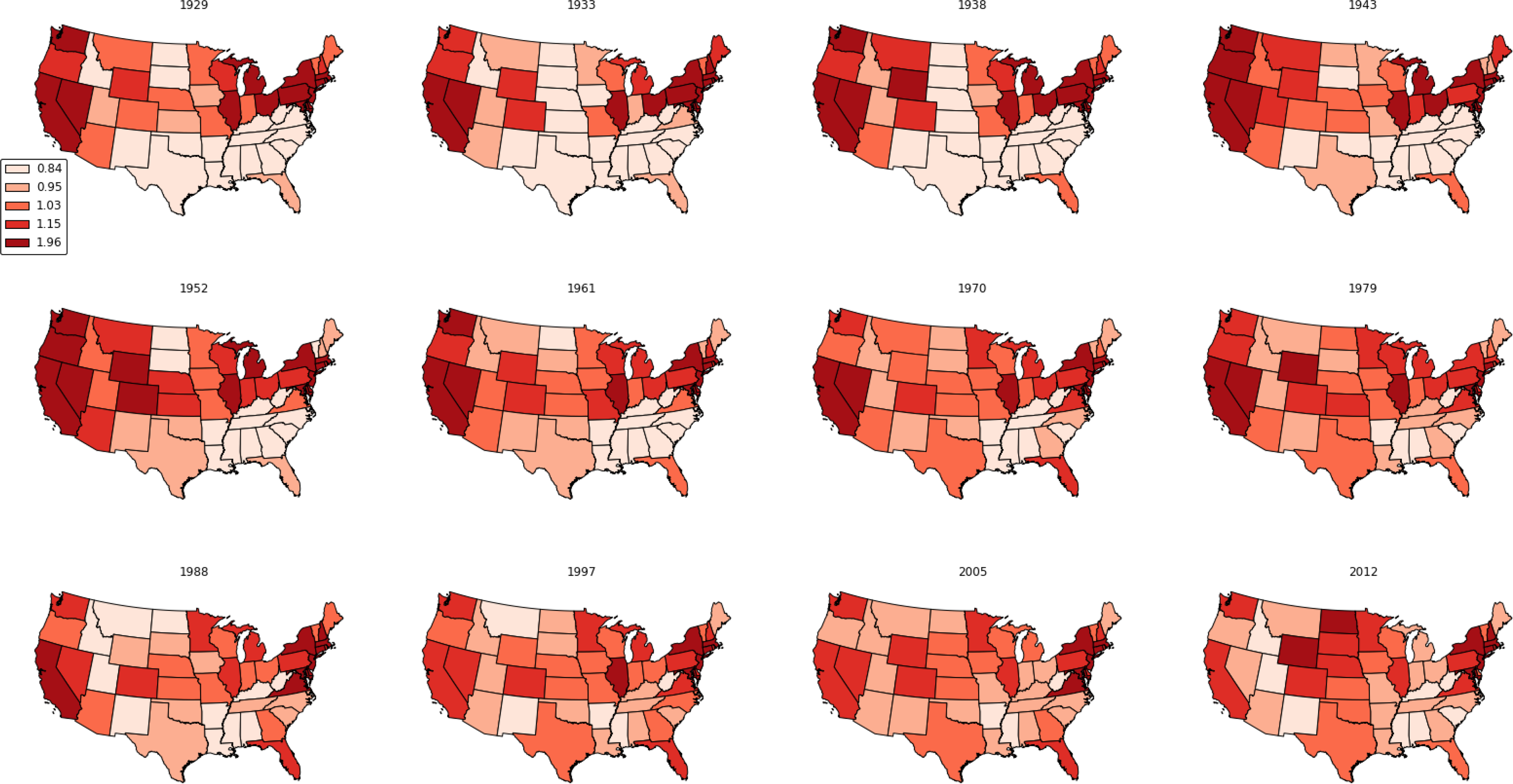
Relative per capita incomes by global quintiles selected years. Legend values are upper bound of each quintile.

The maps provide a rich depiction of the changing structure of personal and spatial income inequality in the United States At the same time, this depiction is a challenge to summarize from a visual perspective. In order to address this challenge, we can turn to a series of formal analytics to provide more specific insights into these complex dynamics.

Homogeneous Inequality Dynamics?

The first set of tests explore the question of whether the different regional series display distinct transitional dynamics over the study period.¹¹

Beginning with the local quintile distributions, Table 1 reports the test of homogeneity in the Markov transition probability matrices between the 0.01 percentile and 0.10 percentile income shares. The test is based on the quintile distribution of the state inequality shares, as measured by the 0.01 share or the 0.10 share. The transition matrix under the null P(H0) is estimated by pooling the two series as a single chain, while the bottom two tables report the marginal transition probability matrices estimated for each share series separately. Both the likelihood ratio and χ² tests are marginally significant (p = .10) and an examination of the diagonal elements of the two marginal tables reveals that the state 0.01 percentile distribution displays relatively greater mobility relative to the distribution based on the 0.10 shares. Given that the 0.01 and 0.10 share series are correlated by construction, in what follows I focus on only the 0.01 shares in comparisons with measures of regional inequality dynamics.

Table 1.

Markov Homogeneity Tests, 0.01 Percentile and 0.10 Percentile Shares, and US State Incomes.

Markov homogeneity test
Number of classes: 5
Number of transitions: 9,216
Number of regimes: 2
Regime names: S01, S10
Test		LR		Q
Stat.		28.629		28.449
DOF		20		20
p value		0.095		0.099
P(H0)	Q0	Q1	Q2	Q3	Q4
Q0	0.809	0.155	0.026	0.006	0.004
Q1	0.172	0.552	0.237	0.031	0.008
Q2	0.025	0.210	0.548	0.190	0.027
Q3	0.010	0.036	0.212	0.582	0.159
Q4	0.001	0.006	0.022	0.152	0.819
P(S01)	Q0	Q1	Q2	Q3	Q4
Q0	0.790	0.176	0.026	0.004	0.004
Q1	0.192	0.547	0.227	0.027	0.007
Q2	0.027	0.198	0.558	0.191	0.026
Q3	0.010	0.034	0.216	0.567	0.172
Q4	0.001	0.003	0.017	0.171	0.808
P(S10)	Q0	Q1	Q2	Q3	Q4
Q0	0.829	0.133	0.026	0.008	0.003
Q1	0.153	0.557	0.248	0.035	0.008
Q2	0.023	0.222	0.537	0.190	0.028
Q3	0.010	0.039	0.207	0.597	0.146
Q4	0.001	0.008	0.027	0.133	0.830

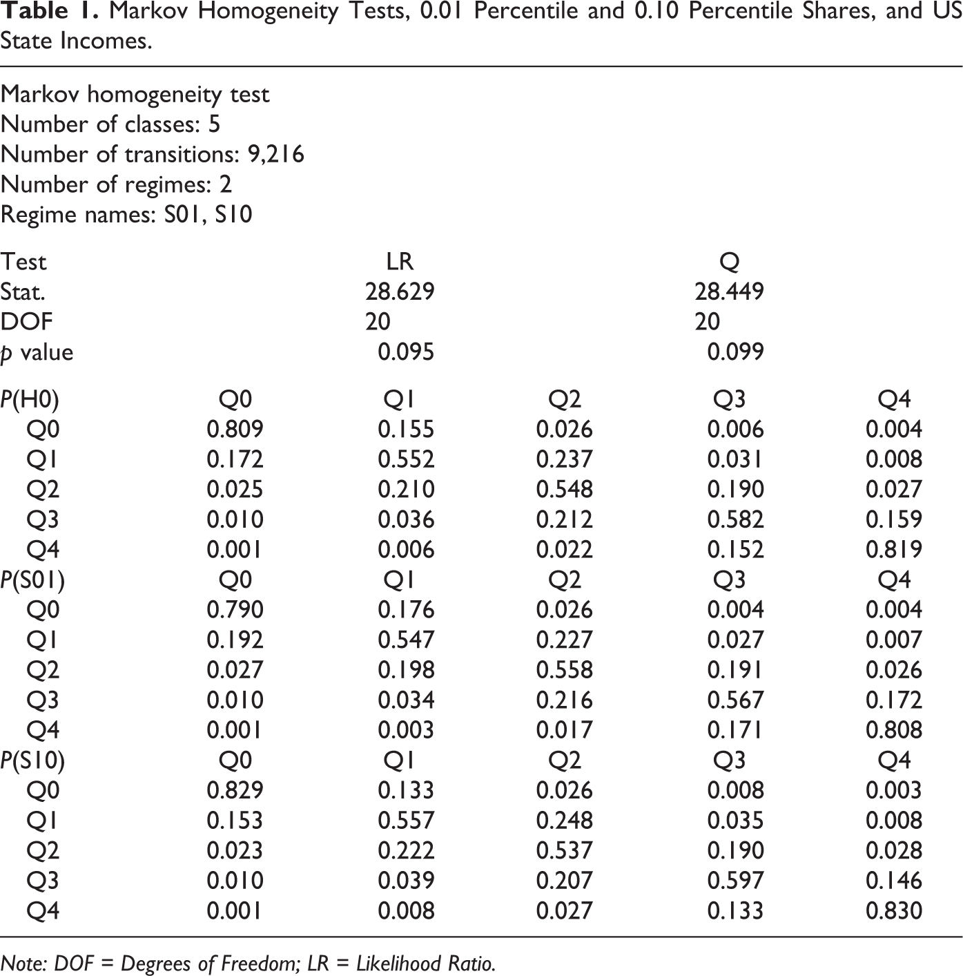
Note: DOF = Degrees of Freedom; LR = Likelihood Ratio.

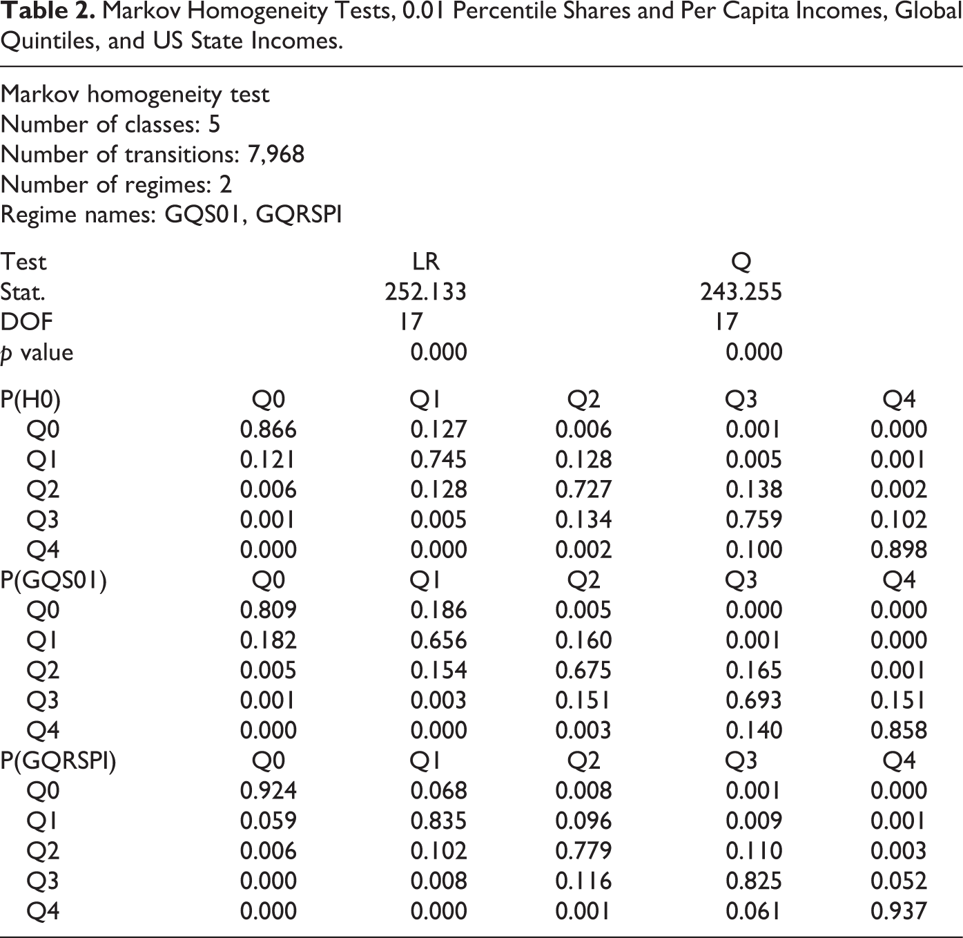
The question of whether the dynamics of interpersonal and regional inequality are distinct is next examined in Table 2 where the estimated Markov transition matrices for the global quintile series for the S01 and relative per capita income series RSPI are tested for homogeneity. Both the likelihood ratio and Q tests of homogeneity are significant.¹² Moreover, the mobility in the S01 series is substantially greater than that in the per capita income series as reflected in the larger diagonal values in the table for the second series.

Table 2.

Markov Homogeneity Tests, 0.01 Percentile Shares and Per Capita Incomes, Global Quintiles, and US State Incomes.

Markov homogeneity test
Number of classes: 5
Number of transitions: 7,968
Number of regimes: 2
Regime names: GQS01, GQRSPI
Test		LR		Q
Stat.		252.133		243.255
DOF		17		17
p value		0.000		0.000
P(H0)	Q0	Q1	Q2	Q3	Q4
Q0	0.866	0.127	0.006	0.001	0.000
Q1	0.121	0.745	0.128	0.005	0.001
Q2	0.006	0.128	0.727	0.138	0.002
Q3	0.001	0.005	0.134	0.759	0.102
Q4	0.000	0.000	0.002	0.100	0.898
P(GQS01)	Q0	Q1	Q2	Q3	Q4
Q0	0.809	0.186	0.005	0.000	0.000
Q1	0.182	0.656	0.160	0.001	0.000
Q2	0.005	0.154	0.675	0.165	0.001
Q3	0.001	0.003	0.151	0.693	0.151
Q4	0.000	0.000	0.003	0.140	0.858
P(GQRSPI)	Q0	Q1	Q2	Q3	Q4
Q0	0.924	0.068	0.008	0.001	0.000
Q1	0.059	0.835	0.096	0.009	0.001
Q2	0.006	0.102	0.779	0.110	0.003
Q3	0.000	0.008	0.116	0.825	0.052
Q4	0.000	0.000	0.001	0.061	0.937

Spatial Mobility Dynamics

Global and local spatial autocorrelation

Figure 7 portrays the time series for the z values of Moran’s I global measure of spatial autocorrelation for the per capita income and one-percent income shares over the period. Relative to the critical value of 1.96 (dotted horizontal line), there are clear differences between the two series with regard to the presence of spatial dependence. For the per capita series, spatial dependence is found each year in the sample displaying a drop from its strongest levels earlier in the series until 1980 at which point the dependence reaches its lowest level. However, even at this minimum the dependence is still significant and following 1980 there is an increase in the strength of spatial dependence. By contrast, the global measure for the one percent income share is never significant during the period 1929–2012. In other words, from a whole map or global perspective, state interpersonal income inequality is randomly distributed in space.

Figure 7.

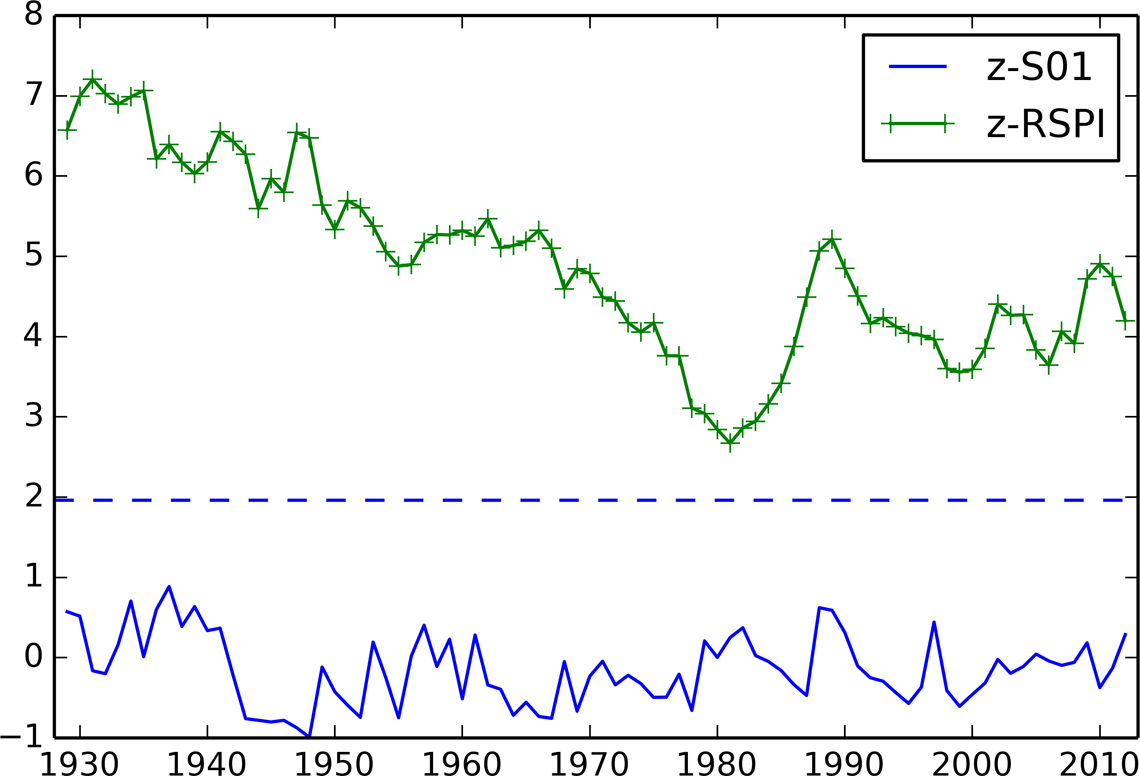
Global spatial autocorrelation, S01 and RSPI, z values Moran’s I, Queen contiguity.

Turning to the local measures, Figure 8 displays the time series of counts for the number of significant local statistics for each series. Now, there is evidence of local clustering despite the finding of no global spatial autocorrelation for S01. At the same time, there is a greater extent of local clustering for RSPI than for S01, reflecting similar finding for the global case. For RSPI, the pattern for the evolution of the number of significant Local Indicator of Spatial Association (LISAs) is roughly in line with the pattern of the global measure.

Figure 8.

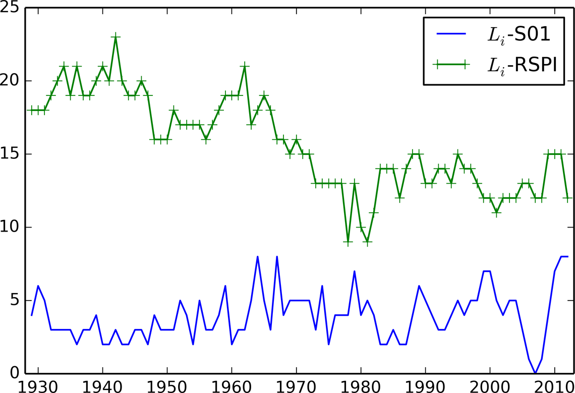
Local spatial autocorrelation, S01 and RSPI, number of significant local Moran’s I values, Queen contiguity.

Table 3 decomposes the total counts from Figure 8 by state and which quadrant of the Moran scatter plot the significant local statistic falls in. For the RSPI series, there are two dominant groups of states, those falling in the high–high (HH) quadrant in the majority of years (562 instances) including the northeastern states (CT, DE, MA, NJ, NY, PA, and RI), and those comprising the low–low (LL) group (675 instances) which includes the southern states (AL, AR, FL, GA, LA, MS, NC, SC, TN, and TX). Less common are the spatial outliers—local statistics falling into either the low–high (LH) or high–low (HL) quadrants.

Table 3.

Local Autocorrelation Statistics by Moran Scatter Plot Quadrant, S01, and RSPI.

State	RSPI					S01
State	NS	HH	LH	LL	HL	NS	HH	LH	LL	HL
AL	24	0	0	60	0	84	0	0	0	0
AZ	76	3	5	0	0	78	0	0	6	0
AR	4	0	0	80	0	83	1	0	0	0
CA	75	9	0	0	0	84	0	0	0	0
CO	76	0	0	0	8	81	0	0	3	0
CT	16	68	0	0	0	64	1	19	0	0
DE	19	65	0	0	0	73	0	0	11	0
FL	48	0	0	31	5	63	0	0	13	8
GA	22	0	0	62	0	83	0	0	1	0
ID	69	3	12	0	0	79	0	0	0	5
IL	84	0	0	0	0	54	24	6	0	0
IN	84	0	0	0	0	76	0	0	1	7
IA	84	0	0	0	0	51	0	33	0	0
KS	84	0	0	0	0	75	0	0	1	8
KY	84	0	0	0	0	75	0	9	0	0
LA	1	0	0	83	0	84	0	0	0	0
ME	84	0	0	0	0	71	1	12	0	0
MD	84	0	0	0	0	71	0	0	3	10
MA	22	62	0	0	0	49	14	21	0	0
MI	84	0	0	0	0	43	5	36	0	0
MN	81	0	0	3	0	73	6	1	0	4
MS	0	0	0	84	0	80	0	0	0	4
MO	72	0	0	9	3	77	0	0	1	6
MT	78	0	0	6	0	84	0	0	0	0
NE	84	0	0	0	0	84	0	0	0	0
NV	82	1	0	1	0	84	0	0	0	0
NH	84	0	0	0	0	82	2	0	0	0
NJ	24	60	0	0	0	84	0	0	0	0
NM	84	0	0	0	0	84	0	0	0	0
NY	9	75	0	0	0	84	0	0	0	0
NC	45	0	0	39	0	83	0	0	1	0
ND	84	0	0	0	0	84	0	0	0	0
OH	76	0	0	8	0	82	0	0	1	1
OK	80	0	0	4	0	84	0	0	0	0
OR	39	45	0	0	0	84	0	0	0	0
PA	10	74	0	0	0	80	0	0	4	0
RI	4	77	3	0	0	84	0	0	0	0
SC	60	0	0	24	0	79	0	0	5	0
SD	82	2	0	0	0	84	0	0	0	0
TN	0	0	0	84	0	84	0	0	0	0
TX	6	0	0	73	5	69	0	3	0	12
UT	84	0	0	0	0	83	0	0	1	0
VT	33	17	34	0	0	70	14	0	0	0
VA	57	0	0	22	5	82	0	0	0	2
WA	84	0	0	0	0	84	0	0	0	0
WV	84	0	0	0	0	83	0	0	1	0
WI	83	1	0	0	0	84	0	0	0	0
WY	82	0	0	2	0	81	0	0	0	3
Total	2715	562	54	675	26	3701	68	140	53	70

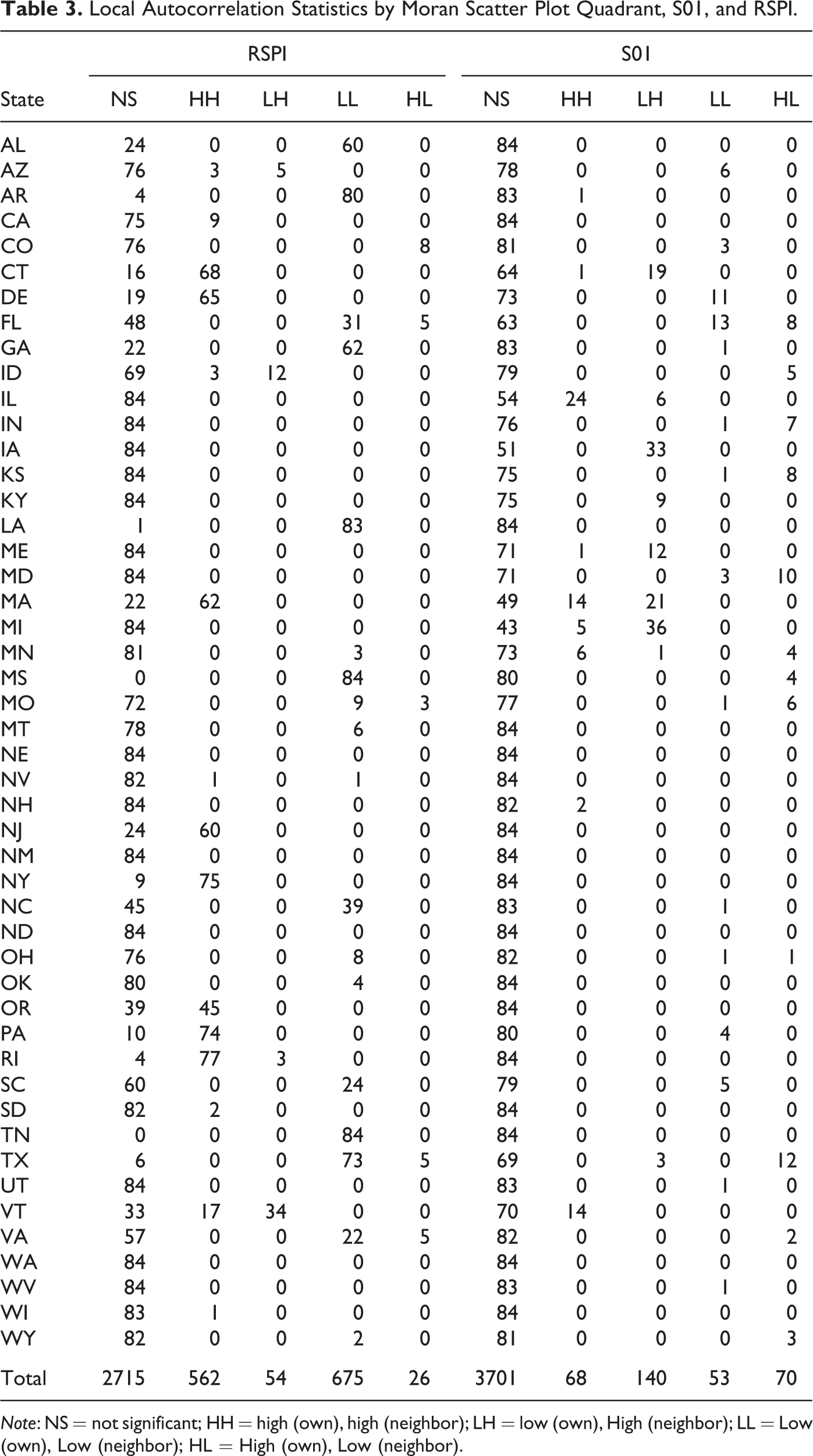
Note: NS = not significant; HH = high (own), high (neighbor); LH = low (own), High (neighbor); LL = Low (own), Low (neighbor); HL = High (own), Low (neighbor).

The pattern for the decomposition of the LISA counts for the one percent shares is less defined than for the RSPI series. Only three states have at least ten LISAs in the HH quadrant—reflecting spatial hot spots of interpersonal inequality, while only two states, FL and DE, fall in the LL quadrant in ten or more years, in this case forming cold spots of income inequality. Moreover, the largest number of LISAs fall in the LH quadrant for the S01 series (140 instances), followed by the HL quadrant (70 instances). In other words, the S01 and RSPI series are distinguished by the former have more local outliers, while the latter having more clusters (hot and cold spots).

Spatial Markov

The results of the spatial Markov tests are reported in Tables 4 and 5 for the S01 and RSPI series, respectively. Recall that the test examines whether the transitional probabilities for the chain are influenced by the level of the spatial lag for the chain at the beginning of the transition period. For both series, the spatial independence assumption is rejected meaning that local context can shape the movement of the chain in the distribution. For example, on average states in the poorest quintile at the beginning of a period have an estimated probability of 0.924 of remaining in that quintile at the end of the year. However, when focusing on states in the first quintile surrounded by neighboring states also in the first quintile, that probability increases to 0.972 percent, while if the neighbors are in the fifth quintile the probability drops to 0.600 (Table 5).

Table 4.

Spatial Markov Test, S01, k = 5.

Spatial Markov test S01
Number of classes: 5
Number of transitions: 3,984
Number of regimes: 5
Regime names: LAG0, LAG1, LAG2, LAG3, LAG4
Test		LR		Q
Stat.		194.130		339.776
DOF		60		60
p value		0.000		0.000
P(H0)	C0	C1	C2	C3	C4
C0	0.809	0.186	0.005	0.000	0.000
C1	0.182	0.656	0.160	0.001	0.000
C2	0.005	0.154	0.675	0.165	0.001
C3	0.001	0.003	0.151	0.693	0.151
C4	0.000	0.000	0.003	0.140	0.858
P(LAG0)	C0	C1	C2	C3	C4
C0	0.816	0.179	0.004	0.000	0.000
C1	0.211	0.729	0.061	0.000	0.000
C2	0.000	0.262	0.714	0.024	0.000
C3	0.167	0.000	0.167	0.500	0.167
C4	0.000	0.000	0.000	0.200	0.800
P(LAG1)	C0	C1	C2	C3	C4
C0	0.833	0.162	0.004	0.000	0.000
C1	0.178	0.639	0.184	0.000	0.000
C2	0.016	0.207	0.717	0.060	0.000
C3	0.000	0.020	0.255	0.667	0.059
C4	0.000	0.000	0.000	0.136	0.864
P(LAG2)	C0	C1	C2	C3	C4
C0	0.646	0.354	0.000	0.000	0.000
C1	0.126	0.615	0.259	0.000	0.000
C2	0.000	0.125	0.667	0.208	0.000
C3	0.000	0.000	0.215	0.718	0.068
C4	0.000	0.000	0.000	0.304	0.696
P(LAG3)	C0	C1	C2	C3	C4
C0	0.857	0.114	0.029	0.000	0.000
C1	0.204	0.537	0.241	0.019	0.000
C2	0.006	0.110	0.686	0.198	0.000
C3	0.000	0.000	0.139	0.711	0.150
C4	0.000	0.000	0.000	0.153	0.847
P(LAG4)	C0	C1	C2	C3	C4
C0	0.800	0.200	0.000	0.000	0.000
C1	0.250	0.375	0.375	0.000	0.000
C2	0.000	0.273	0.424	0.273	0.030
C3	0.000	0.005	0.087	0.647	0.261
C4	0.000	0.000	0.004	0.121	0.875

Table 5.

Spatial Markov Test, RSPI, k = 5.

Spatial Markov test RSPI
Number of classes: 5
Number of transitions: 3,984
Number of regimes: 5
Regime names: LAG0, LAG1, LAG2, LAG3, LAG4
Test		LR		Q
Stat.		173.190		195.109
DOF		64		64
p value		0.000		0.000
P(H0)	C0	C1	C2	C3	C4
C0	0.924	0.068	0.008	0.001	0.000
C1	0.059	0.835	0.096	0.009	0.001
C2	0.006	0.102	0.779	0.110	0.003
C3	0.000	0.008	0.116	0.825	0.052
C4	0.000	0.000	0.001	0.061	0.937
P(LAG0)	C0	C1	C2	C3	C4
C0	0.972	0.026	0.002	0.000	0.000
C1	0.051	0.803	0.139	0.007	0.000
C2	0.009	0.151	0.717	0.123	0.000
C3	0.000	0.024	0.262	0.619	0.095
C4	0.000	0.000	0.000	0.286	0.714
P(LAG1)	C0	C1	C2	C3	C4
C0	0.777	0.182	0.033	0.008	0.000
C1	0.074	0.860	0.062	0.004	0.000
C2	0.000	0.103	0.806	0.091	0.000
C3	0.000	0.000	0.072	0.892	0.036
C4	0.000	0.000	0.000	0.195	0.805
P(LAG2)	C0	C1	C2	C3	C4
C0	0.844	0.156	0.000	0.000	0.000
C1	0.063	0.844	0.076	0.013	0.004
C2	0.016	0.089	0.801	0.089	0.005
C3	0.000	0.006	0.091	0.835	0.068
C4	0.000	0.000	0.000	0.132	0.868
P(LAG3)	C0	C1	C2	C3	C4
C0	0.948	0.039	0.013	0.000	0.000
C1	0.045	0.836	0.109	0.009	0.000
C2	0.000	0.073	0.794	0.129	0.004
C3	0.000	0.018	0.189	0.732	0.061
C4	0.000	0.000	0.005	0.071	0.924
P(LAG4)	C0	C1	C2	C3	C4
C0	0.600	0.400	0.000	0.000	0.000
C1	0.030	0.773	0.182	0.015	0.000
C2	0.010	0.136	0.728	0.126	0.000
C3	0.000	0.005	0.094	0.865	0.036
C4	0.000	0.000	0.000	0.023	0.977

For the income shares, on average, states with the highest levels of interpersonal inequality have a 0.858 probability of remaining in the fifth quintile if they began a year in that quintile. However, if a state in the fifth quintile of interpersonal income inequality is surrounded by states that are on average also in that quintile the probability increases to 0.875 (Table 4). In contrast to the cross-sectional setting where spatial dependence in the income shares was found to be weak or nonexistent in most years, the dynamics of state personal income inequality are sensitive to spatial context as the assumption of one transition matrix applying across all observations is rejected.

Discussion and Conclusion

Using the US states over the period 1929–2012, this article has examined two of Alonso’s five bells with a particular focus on their space–time coevolution. Application of exploratory space–time analytics reveals that the patterns of social, or interpersonal, and regional, or interregional, inequality are complex and display characteristics that were not considered in Alonso’s original stylized model. Interpersonal inequality displayed a U pattern resulting in levels of inequality at the end of the period actually exceeding the alarmingly high values found in the 1920s. By contrast, interregional income inequality between the US states has displayed a general decline up until the end of this period where convergence has slowed or even reversed.

In addition to the differences in the overall trends for the two types of inequality, their distributional dynamics are also found to be distinct with social inequality exhibiting greater mobility than interregional inequality, meaning that states move across the quintiles of the social inequality distribution more frequently than they do in the per capita income distribution.

The spatial patterns of these movements are also differentiated as per capita incomes are strongly spatially autocorrelated each year in the sample, while global spatial dependence is never found for social inequality. A local analysis, however, reveals evidence of pockets of hot and cold spots for interregional inequality as well as spatial outliers for social inequality. Finally, spatial Markov tests reveal that the transitional dynamics for both series are not independent of the local context for a state economy as the estimated transition probability matrices for both social and interregional income inequality are found to be significantly different across regimes defined on the spatial lag of each series.

Alongside the distinct spatial patterns of interregional and interpersonal inequality are pronounced temporal differences in the spatial distribution of interpersonal inequality. The two periods of high interpersonal inequality, the 1920’s and the post-1980 era, have substantially different spatial distributions with the latter distribution characterized by a spatial homogenization of high personal income inequality, while in the former period high interpersonal income inequality is more spatially concentrated along the northeastern and western states.

This homogenization of interpersonal income inequality has also coincided with a reversal of a long running trend toward regional income convergence. The causes of this reversal and its association with increasing interpersonal income inequality are poorly understood. Fan and Casetti (1994) argue that the Rustbelt-Sunbelt shift dominated the US economic landscape up until the late 1960s and was a major force in driving regional income convergence. Subsequently, sectoral shifts reflected in the loss of manufacturing jobs and their replacement with lower paying service resulted in a hollowing out of the personal income distribution. They suggest that the spatial impact of this restructuring may have been uneven with new service and financial sector growth being more prevalent in the traditional core.

In addition to deindustrialization, fiscal policies and political decentralization associated with the Reagan administration have been suggested as possible causes for increasing interregional inequality. Coughlin and Mandelbaum (1988) found that defense expenditures during the Reagan administration were spatially biased toward high-income states and away from low-income states, increasing interstate inequality.

The decentralization associated with Reagan’s New Federalism gave individual states more freedom to shape economic development policies. Decentralization could have led to greater spatial inequalities through a variety of mechanisms such as lost economies of scale in addressing concentrated poverty and differences in institutional capacities and resources across regions, although the relationship between decentralization and spatial inequality may vary depending on the level of development of a nation (Rodríguez-Pose and Ezcurra 2010).

At the same time, the trend toward spatially ubiquitous levels of high personal income inequality uncovered in the latter period of this study may suggest that policies at the national level, such as tax reforms (Stiglitz 2014), and macroeconomic events—including the great recession, financial meltdown, and housing market implosion—have had global effects resulting in greater inequality due to declining real incomes at the bottom and middle of the income distribution and the rise of private debt in the form of loans leveraging ephemeral house price increases (Essletzbichler 2015; Galbraith 2012).

Although the housing market bubble appeared to have global impacts in terms of increasing interpersonal income inequality, there is some evidence to suggest that it may have also slowed regional convergence. Ganong and Shoag (2015) argue that high housing costs in high-income regions worked to dampen migration of low-wage workers from poor to richer regions due to the price sensitivity of low-income workers. This reduced the labor and human capital reallocation process that historically had been an engine of regional convergence in the United States. In short, the returns to residing in productive regions net of housing costs have moved in opposite directions attracting skilled works but diverting in-migration of unskilled workers. The housing bubble and housing regulations are the argued causes of these house price changes.

The joint consideration of interpersonal inequality and interregional inequality reveals insights that could have implications for regional economic development polices. The greater mobility in interpersonal inequality, relative to average state incomes, suggests that polices may have more impact on reducing (or increasing) inequality within states than they do on relative state income growth. At the same time, the strong evidence of spatial dependence in the dynamics of both inequality series implies that states should not be considered independent actors as policies adopted by one state may have spillover impacts into neighboring states. Taking these policy spillovers into account would argue for a national or regional perspective on state economic development policies.

Application of exploratory space–time methods is a first step toward the call for the “simultaneous consideration” (Alonso 1980, 5) of interpersonal and interregional income inequality dynamics, and a more complete understanding of the dynamics of different types of inequality and their interdependencies. The empirical patterns uncovered here need to be considered from the lenses of existing regional inequality theory and personal income inequality theory with an eye toward their integration. Additionally, from a methodological point of view, the role of spatial context in the dynamics of both social and regional inequality needs to be taken into account in future econometric work.

Footnotes

Acknowledgments

An earlier version of this article was presented at the sixty-first Annual North American Meetings of the Regional Science Association International. I thank Eveline S. van Leeuwen, Rachel Franklin, and the referees for insightful comments on this work. Any errors that remain are mine alone.

Declaration of Conflicting Interests

The author(s) declared no potential conflicts of interest with respect to the research, authorship, and/or publication of this article.

Funding

The author(s) disclosed receipt of the following financial support for the research, authorship, and/or publication of this article: This research was supported in part by the National Science Foundation under Grant SES-1421935.

Notes

References

Alonso

1980. “Five Bell Shapes in Development.” Papers in Regional Science 45:5–16.

Amos

1983. “The Relationship betwen Personal Income Inequality, Regional Income Inequality, and Development.” Regional Science Perspectives 13:3–14.

Amos

1988. “Unbalanced Regional Growth and Regional Income Inequality in the Latter Stages of Development.” Regional Science and Urban Economics 18:549–66.

Andersson

Klaesson

Larsson

J. P.

. 2014. “The Sources of the Urban Wage Premium by Worker Skills: Spatial Sorting or Agglomeration Economies?” Papers in Regional Science 93:727–47.

Anselin

1995. “Local Indicators of Spatial Association-LISA.” Geographical Analysis 27:93–115.

Barro

R. J.

Sala-i Martin

. 1991. “Convergence across States and Regions.” Brookings Papers on Economic Activity 1991:107–82.

Bernard

Jones

. 1996. “Productivity and Convergence across us States and Industries.” Empirical Economics 21:113–35.

Bickenbach

Bode

. 2003. “Evaluating the Markov Property in Studies of Economic Convergence.” International Regional Science Review 26:363–92.

Bowles

Durlauf

S. N.

Hoff

. 2008. Poverty Traps. Princeton, NJ: Princeton University Press.

10.

Breau

2007. “Income Inequality across Canadian Provinces in an Era of Globalization: Explaining Recent Trends.” The Canadian Geographer 51:72–90.

11.

Card

DiNardo

J. E.

. 2002. “Skill Biased Technological Change and Rising Wage Inequality: Some Problems and Puzzles.” Journal of Labor Economics 20:733–83.

12.

Chakravorty

1996. “Urban Inequality Revisited—The Determinants of Income Distribution in U.S. Metropolitan Areas.” Urban Affaris Review 31:759–77.

13.

Chatterji

Dewhurst

J. H. L. L.

. 1996. “Convergence Clubs and Relative Economic Performance in Great Britan.” Regional Studies 30:31–40.

14.

Coughlin

C. C.

Mandelbaum

T. B.

. 1988. “Why Have State Per-capita Incomes Diverged Recently?” Review of the Federal Reserve Bank of St. Louis 70:24–36.

15.

Easterlin

1960. “Regional Growth of Income.” In Population Redistribution and Economic Growth in the United States, 1870-1950, edited by Kuznets

Miller

Easterlin

, 141–203. Philadelphia, PA: American Philosophical Society.

16.

Essletzbichler

2015. “The Top 1% in US Metropolitan Areas.” Applied Geography 61:35–46.

17.

Fan

C. C.

Casetti

. 1994. “The Spatial and Temporal Dynamics of US Regional Income Inequality, 1950–1989.” The Annals of Regional Science 28:177–96.

18.

Frank

M. W.

2009. “Inequality and Growth in the United States: Evidence from a New State-level Panel of Income Inequality Measures.” Economic Inquiry 47:55–68.

19.

Galbraith

J. K.

2012. Inequality and Instability: A Study of the World Economy Just Before the Great Crisis. Oxford, UK: Oxford University Press.

20.

Ganong

Shoag

. 2015. “Why Has Regional Income Convergence in the US Declined?” Working Paper no. RWP12-028. Cambridge, MA: Kennedy School, Harvard University.

21.

Gordon

2014. Growing Apart: A Political History of American Inequality. Washington, DC: Institute for Policy Studies.

22.

Janikas

M. V.

Rey

S. J.

. 2005. “Spatial Clustering, Inequality, and Income Convergence.” Région et Développement 25:41–64.

23.

Janikas

M. V.

Rey

S. J.

. 2008. “On the Relationship between Spatial Clustering, Inequality, and Economic Growth in the United States: 1969-2000.” Région et Développement 27:13–34.

24.

Kristal

2013. “The Capitalist Machine: Computerization, Workers’ Power, and the Decline in Labor’s Share within US Industries.” American Sociological Review 78:361–89.

25.

Krugman

P. R.

1991. Geography and Trade. Cambridge, MA: MIT press.

26.

Krugman

P. R.

Lawrence

. 1993. “Trade, Jobs, and Wages.” Technical report. Cambridge, MA: National Bureau of Economic Research.

27.

Kuznets

1955. “Economic Growth and Income Equality.” American Economic Review 45:1–28.

28.

Leamer

E. E.

1994. “Trade, Wages and Revolving Door Ideas.” Technical report. Cambridge, MA: National Bureau of Economic Research.

29.

Levernier

Rickman

D. S.

Partridge

M. D.

. 1995. “Variation in US State Income Inequality: 1960-1990.” International Regional Science Review 18:355–78.

30.

Levy

Murnane

R. J.

. 1992. “US Earnings Levels and Earnings Inequality: A Review of Recent Trends and Proposed Explanations.” Journal of Economic Literature 30:1333–81.

31.

Madden

J. F.

2000. Changes in Income Inequality within US Metropolitan Areas. Kalamazoo, MI: WE Upjohn Institute.

32.

Metwally

M. M.

Jensen

R. C.

. 1973. “A Note on the Measurement of Regional Income Dispersion.” Economic Development and Cultural Change 22:135–36.

33.

Moretti

2013. “Real Wage Inequality.” American Economic Journal 5:65–103.

34.

Myrdal

1957. Rich Lands and Poor. New York: Harper.

35.

Nielsen

Alderson

A. S.

. 1997. “The Kuznets Curve and the Great U-turn: Income Inequality in US Counties, 1970 to 1990.” American Sociological Review 62:12–33.

36.

Noah

2012. The Great Divergence: America’s Growing Inequality Crisis and What We Can Do About It. New York: Bloomsbury Publishing USA.

37.

Odland

Ellis

. 2001. “Changes in the Inequality of Earnings for Young Men in Metropolitan Labor Markets, 1979–1989: The Effects of Declining Wages and Sectoral Shifts within an Efficiency Wage Framework.” Economic Geography 77:148–79.

38.

Panizza

2002. “Income Inequality and Economic Growth: Evidence from American Data.” Journal of Economic Growth 7:25–41.

39.

Partridge

J. S.

Partridge

M. D.

Rickman

D. S.

. 1998. “State Patterns in Family Income Inequality.” Contemporary Economic Policy 16:277–94.

40.

Partridge

M. D.

1997. “Is Inequality Harmful for Growth? Comment.” The American Economic Review 87:1019–32.

41.

Partridge

M. D.

2005. “Does Income Distribution Affect U.S. State Economic Growth?” Journal of Regional Science 45:363–94.

42.

Piketty

Saez

. 2006. “The Evolution of Top Incomes: A Historical and International Perspective.” Technical report. Cambridge, MA: National Bureau of Economic Research.

43.

Piketty

Saez

. 2013. “Top Incomes and the Great Recession: Recent Evolutions and Policy Implications.” IMF Economic Review 61:456–78.

44.

Rey

S. J.

2001. “Spatial Empirics for Economic Growth and Convergence.” Geographical Analysis 33:195–214.

45.

Rey

S. J.

2004. “Spatial Analysis of Regional Income Inequality.” In Spatially Integrated Social Science: Examples in Best Practice, edited by Goodchild

Janelle

, 280–99. Oxford, UK: Oxford University Press.

46.

Rey

S. J.

2014. “Spatial Dynamics and Space-time Data Analysis.” In Handbook of Regional Science edited by Fischer

M. M.

Nijkamp

, 1365–83. Berlin, Germany: Springer.

47.

Rey

S. J.

2015. “Discrete Regional Distribution Dynamics Revisited.” Journal of Regional and Urban Economics 7:83–104.

48.

Rey

S. J.

Anselin

. 2010. “PySAL: A Python Library of Spatial Analytical Methods.” In Handbook of Applied Spatial Analysis, edited by Fischer

M. M.

Getis

, 175–93. Berlin, Germany: Springer.

49.

Rey

S. J.

Dev

. 2006. “σ-convergence in the Presence of Sspatial Effects.” Papers in Regional Science 85:217–34.

50.

Rey

S. J.

Janikas

M. V.

. 2005. “Regional Convergence, Inequality and Space.” Journal of Economic Geography 5:155–76.

51.

Rey

S. J.

Le Gallo

. 2009. “Spatial Analysis of Economic Convergence.” In Handbook of Econometrics Volume II: Applied Econometrics, edited by Mills

T. C.

Patterson

, 1251–90. New York: Palgrave Macmillan.

52.

Rey

S. J.

Montouri

B. D.

. 1999. “U.S. Regional Income Convergence: A Spatial Econometric Perspective.” Regional Studies 33:145–56.

53.

Rietveld

1991. “A Note on Interregional Versus Intraregional Inequality.” Regional Science and Urban Economics 21:627–37.

54.

Rigby

Breau

. 2008. “Impacts of Trade on Wage Inequality in Los Angeles: Analysis Using Matched Employer–Employee Data.” Annals of the Association of American Geographers 98:920–40.

55.

Rodríguez-Pose

2012. “Trade and Regional Inequality.” Economic Geography 88:109–36.

56.

Rodríguez-Pose

Ezcurra

. 2010. “Does Decentralization Matter for Regional Disparities? A Cross-country Analysis.” Journal of Economic Geography 10:619–44.

57.

Sachs

J. D.

Shatz

H. J.

Deardorff

Hall

R. E.

. 1994. “Trade and Jobs in US Manufacturing.” Brookings Papers on Economic Activity 1994:1–84.

58.

Shorrocks

Wan

. 2005. “Spatial Decomposition of Inequality.” Journal of Economic Geography 5:59–81.

59.

Smeeding

T. M.

Thompson

J. P.

. 2011. “Recent Trends in Income Inequality.” Research in Labor Economics 32:1–50.

60.

Stiglitz

J. E.

2012. The Price of Inequality. London, UK: Penguin.

61.

Stiglitz

J. E.

2014. Reforming Taxation to Promote Growth and Equity. New York, NY: Roosevelt Institute.

62.

Wilkinson

R. G.

Pickett

K. E.

. 2006. “Income Inequality and Population Health: A Review and Explanation of the Evidence.” Social Science & Medicine 62:1768–84.

63.

Williamson

1965. “Regional Inequality and the Process of National Development.” Economic Development and Cultural Change 13:3–47.

64.

Wood

1994. North-south Trade, Employment and Inequality: Changing Fortunes in a Skill-driven World. New York: Oxford University Press.

65.

Young

Higgins

Levy

. 2008. “Sigma Convergence Versus Beta Convergence: Evidence from US County-level Data.” Journal of Money, Credit and Banking 40:1083–93.