The Changes of Urban Structure and Commuting: An Application to Metropolitan Statistical Areas in the United States

Abstract

While urban structures have been delineated at the regional level, few works have explored the impact of urban structures on commuting at this same level. This article studies how urban structures affect commuting from 2000 to 2010. It applies a spatial statistical tool, standard deviation ellipses, to capture spatial patterns of jobs and residential workers for metropolitan statistical areas (MSAs). Two urban structure indexes are constructed to illustrate different decentralization levels of employment with reference to the distribution of residential workers; one illustrates the spatial decentralization of high job density nodes, while the other shows the spatial decentralization of moderate job density nodes. Commuting times of two modes by private cars and public transit are analyzed along with the number of commuters. The results highlight three findings: (1) MSAs become more compact in terms of employment distribution, (2) more decentralized high-density nodes lead to less total commuting times, and on the other hand, more decentralized moderate job density nodes contribute to longer commuting times, and (3) the decentralization of high job density nodes is associated with less commuting time of private cars, while they have insignificant effect on commuting time of public transit.

Keywords

urban structure commuting mode standard deviation ellipses workers jobs employment

Introduction

Several studies identified an association between urban structures and commuting; however, there is no unanimous consensus about how and to what extent urban structures influence commuting (Cervero and Wu 1998; Coevering and Schwanen 2006; Horner 2007; Wachs et al. 1993). When analyzing the relationship between urban structures and commuting, a critical part is how to delineate urban structures. Several studies delineate urban structures at micro levels, employing street connectivity, walkability, mixed land use, and residential density (Ewing, Pendall, and Chen 2003; Handy 1996; Scholossberg et al. 2006; Zegras 2004; Zhang 2004), while other studies focus on macrolevels in light of distribution of population, job centers, distance from central business district (CBD), job-to-resident ratios, job proximity, excess commuting, and percentage of employees working in urban cores (Cervero 1996; Giuliano and Small 1991; Hu and Wang 2016; Kim, Sang, and Ban 2014; Ma and Banister 2007; Sohn 2005; F. Wang 2000; Yang et al. 2012). Due to different descriptions of urban structures, previous studies show mixed results about how urban structures influence commuting patterns. For example, Gordon, Richardson, and Wong (1986) explored urban form of Los Angeles by applying the Wright coefficient, claiming that dispersed urban form led to short trips, while Cervero and Wu (1998) analyzed urban structures through identifying the dispersion of employment centers in San Francisco, suggesting that decentralized employment centers were not associated with shorter average commuting distance and time. Other researchers also exemplified the paradox with regard to the impact of urban structures on commuting (Cervero and Wu 1997; Schwanen, Dieleman, and Dijst 2004; Vandersmissen, Villeneuve, and Theriault 2003). These debates exist, on one hand, because ways to define urban structures are different. On the other hand, it is because few studies analyze the impact of urban structures on commuting with a sufficient number of metropolitan areas. Although a couple of papers explored urban structures of all US metropolitan areas, they did not examine the implication of urban structures on commuting patterns (Arribas-Bel and Sanz-Gracis 2014; Hajrasouliha and Hamidi 2017).

To overcome the gap by previous studies, this article proposes a measure for delineating urban structures at the metropolitan level and revisits the effect of urban structures on commuting time across metropolitan statistical areas (MSAs), from 2000 to 2010. Commuting time rather than commuting distance is used because given a fixed distance, depending on different traffic conditions, commuting time varies remarkably and influences commuting patterns greatly (Gordon, Richardson, and Jun 1991). The remainder of this article is organized as follows: second section reviews the literature on urban structures and the impact of urban structures on commuting; third section introduces study areas and data sources; fourth section provides a measure to delineate urban structures by applying standard deviation ellipses (SDEs); fifth section focuses on the impact of urban structures on commuting among the MSAs; and sixth section summarizes the findings and discusses future research.

Urban Structure and Commuting

Alonso’s (1964) monocentric model, centered on a single central business district (CBD), has been one of the most influential depictions of urban structures (Figure 1a). Later, researchers extended this model to describe spatial structures of activities within urban areas, such as transportation, industries, residences, and agriculture (Mills 1972; Muth 1969). Since the 1950s, however, many metropolises in the United States have changed from monocentric to polycentric, with employment centers extending to suburban areas, beyond urban cores (Guiliano and Small 1993; Yang et al. 2012). Studies looking at European cities also claimed that polycentric urban structures denoted the existence of multiple employment subcenters (Aguilera and Mignot 2004; Batty 2001; Bogart and Ferry 1999; Deileman and Faludi 1998; Greene 1980; Kloosterman and Musterd 2001; Parr 2004; Small and Song 1994). Garreau (1991) coined a term, “edge city,” to portray the formation of multiple employment subcenters. According to his research, most edge cites were formed close to existing or planned freeway intersections or along railways and were likely to develop near major airports. In particular, Giuliano and Small (1991) investigated subcenters in the Los Angeles region using 1980 Census journey-to-work data and identified thirty-two centers, with four main centers and twenty-eight subcenters, among which five subcenters are close to airports. Cervero and Wu (1997) studied the San Francisco Bay area and found a distinct polycentric metropolitan form, with three tiers of hierarchical employment centers encircling downtown San Francisco, the primary center. Studies on Chicago also found main centers and employment subcenters located around main centers or the O’Hare Airport (McDonald 1987; F. Wang 2000). All these studies delineate polycentric urban structures with main centers as well as significant subcenters (Figure 1b).

Figure 1.

Urban structure diagram.

A different school of thought provides another description of urban structures. Gordon and Richardson (1996) analyzed the distribution of employment among subcenters in Los Angeles and found the proportion of regional jobs in all subcenters was small and fell from year to year. They suggested Los Angeles might be more accurately described as dispersed rather than polycentric. In a similar analysis, Fuji and Hartshorn (1995) found scattered employment sites in Atlanta. Lang (2003) proposed a term “edgeless city” and pointed out a new suburban form, generalized dispersion, which continued to spread. Garcia-Lopez and Muniz (2010) argued that polycentricity was just an intermediate stage between monocentricity and a more unstructured, chaotic, and amorphous location model, termed scatteration. These studies describe urban structures as generalized dispersion or scatteration (Shearmur et al. 2007), with employment sites scattered in MSAs (Figure 1c).

Along with studies about urban structures, interests in analyzing the impact of urban structures on commuting flourished, specifically, focusing on whether polycentricity or generalized dispersion led to less commuting time or commuting distance. Studies support decentralization leading to less commuting time and/or distance traveled, by arguing that employment subcenters bring jobs to suburban areas, which not only shortens the commuting distance for workers who live close to the subcenters but also saves time for those commuting to the employment subcenters, because they avoid commuting to CBDs during peak hours, when main traffic routes are heavily congested. Gordon, Richardson, and Jun (1991) explored the relationships between urban structures and commuting for the twenty largest MSAs, concluding that during the study period, the average trip times either fell by statistically significant amounts or remained the same. Given the selected MSAs became more polycentric during the study period, so they suggested that polycentric or dispersed metropolitan structures facilitated shorter times. From a spatial perspective, Cervero and Wu (1997) analyzed the commuting time of workers in the San Francisco Bay area, finding commutes made by the employees of suburban centers were shorter in duration than those made by workers traveling to larger and denser urban centers. Yang et al. (2012) analyzed the changes of urban structures and its impact on commuting time from 1970 to 2000 using population data instead of jobs for top fifty MSAs (by population size in 2000). They concluded that decentralization of high-density nodes led to less commuting time, while decentralization of moderate density nodes led to longer commuting time. They, however, failed to analyze the distribution of employment, which was thought as one of the factors that shaped urban structures (Frank et al. 2008; Veneri 2010).

To the contrary, other studies argue that decentralized employment does not satisfy workers’ needs since not all workers’ residences are located close to their adjacent employment centers. Thus, cross-suburb commuting generates longer commuting. At the same time, the growth of dual wage earners in a household makes residential choices complex. These wage earners either choose a residence in the middle of the two workplaces or reside adjacent to one workplace, with little effect on the overall commuting time. Other factors, such as school districts, housing cost, and supply, all affect workers’ choices for residences and thus exert influences on commuting. For example, Cervero and Wu (1998) explored the San Francisco Bay area from 1980 to 1990, showing that employment decentralization had not been associated with shorter average commute distances or durations; Schwanen, Dielenman, and Dijst (2004) used a multilevel approach to analyze commuting behaviors in the Netherlands, suggesting that commuting time for auto drivers was longer in most polycentric regions than in monocentric urban areas. Similarly, analysis in Quebec City indicated, by controlling travel modes and key social factors (i.e., job types, the number of cars in a household), the shift from a monocentric form to a dispersed city form was responsible for increasing commuting time (Vandersmissen, Villeneuve, and Theriault 2003). Melo, Graham, and Noland (2012) studied how urban structure and transport supply affected the distance decay of commuting trips in England and Wales, finding the more monocentric and centralized spatial urban structures were much sensitive to commuting distance which reflected a higher proportion of short distance commutes.

Different from supporting or opposing employment decentralization, several studies hold the idea that polycentricity has little effect on commuting. Coevering and Schwanen (2006) explored thirty-one larger metropolises in Europe, Canada, and the United States. They found that decentralized urban structure either increased commuting time or decreased commuting distance inconsistently, and the urban structure was not the only factor to be statistically related to metropolitan-wide travel patterns. Ma and Banister (2007) delineated urban structures by excess commuting, analyzed urban spatial changes for British cities, and concluded that urban decentralization could lead to either an increase or a decrease in average commuting distance. Chowdhury, Scott, and Kanaroglou (2013) modified Brotchie’s urban triangle to represent maximum and minimum commuting distance to demonstrate urban form of three Canadian cities (Hamilton, Halifax, and Vancouver). They substituted land-use dispersal index for jobs–housing dispersal index to represent urban form and explored the connection between urban structures and commuting distance. Based on their analysis, they found inconsistent relationship between commuting behavior and urban form.

When exploring the connection between urban structures and commuting patterns, all aforementioned efforts assume homogenous wage groups. However, variances of commuting time and/or distances among different wages are important factors to understand the link between urban structure and commuting time and/or distance. Previous literature, by and large, came to a consensus that low-income commuters travel shorter distance than those with higher incomes (Hu, Wang, and Wilmot 2016; Kim et al. 2012; Li 2010; Niedzielski and Boschmann 2014; Sultana 2002; E Wang, Song, and Xu 2011), while opinions diverged on the link between income and commuting time (Blumenberg and Manville 2004; Sermons and Koppelman 2001; D Wang and Chai 2009). Other perspectives, involving the role of urban structure in shaping commuting patterns for different occupations, genders, races, and commuting modes, also attract research interests (Crane 2007; Horner and Mefford 2007; Ibipo 1995; Kwan and Kotsev 2015; Kawase 2004; Kim et al. 2012; Mauch and Taylor 1997; McLafferty 1997; Murphy 2009; O’Kelly, Niedzielski, and Gleeson 2012; Sang, O’Kelly, and Kwan 2011; Waddell 1992). These literatures found the black and women commuted shorter than the white and men. Commuting distance or/and time varied a lot among different occupations. Study areas of these works generally focus on one city, county, or MSA. Since we aim to explore how urban structures shape commuting patterns in a macro view across MSAs, we do not go into details in terms of wage groups, occupations, genders, or races.

When considering characteristics of commuters as homogenous, we found empirical results from previous research have been distinctly different in the role of urban structures in shaping commuting patterns. These differences ascribe to factors, such as the selection of study areas and descriptions of urban structures. A small number of MSAs hardly get a comprehensive picture about how urban structures affect commuting, while different descriptions of urban structures, such as monocentric, polycentric, or generalized dispersed, lead to different conclusions regarding the impact of urban structure. To add an extensive perspective for urban structures, we propose a measure to quantify different degrees of employment distribution with reference to the distribution of residences across MSAs in United States.

Study Area and Data

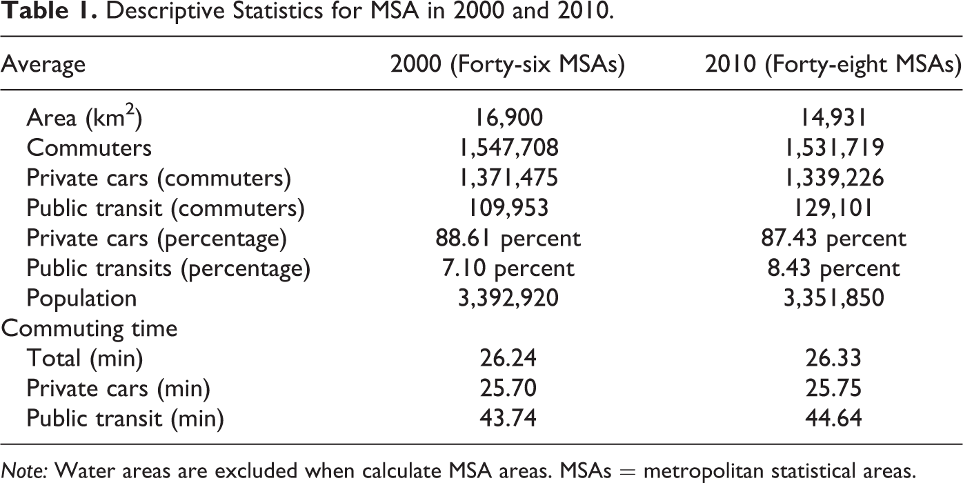
MSA is a geographical region with a relatively high population density at its core and close economic ties through the area (Office of Management and Budget 2010). We select MSAs with more than 500,000 commuters as study areas, since a large number of commuters have potential to form complex commuting flows, and we aim to see how these flows are affected by urban structures. Among all MSAs, forty-six MSAs in 2000 and forty-eight MSAs in 2010 are selected (Table 1).

Table 1.

Descriptive Statistics for MSA in 2000 and 2010.

Average	2000 (Forty-six MSAs)	2010 (Forty-eight MSAs)
Area (km²)	16,900	14,931
Commuters	1,547,708	1,531,719
Private cars (commuters)	1,371,475	1,339,226
Public transit (commuters)	109,953	129,101
Private cars (percentage)	88.61 percent	87.43 percent
Public transits (percentage)	7.10 percent	8.43 percent
Population	3,392,920	3,351,850
Commuting time
Total (min)	26.24	26.33
Private cars (min)	25.70	25.75
Public transit (min)	43.74	44.64

Note: Water areas are excluded when calculate MSA areas. MSAs = metropolitan statistical areas.

Boundaries of MSAs changed significantly from 2000 to 2010 (Figure 2). In 2000 and 2010, the Office of Management and Budget defined an MSA by first selecting a central county/counties, and then, combined the adjacent county/counties with an MSA if (1) at least 25 percent of the employed residents of the potential outlying county worked in the MSA’s central county/counties or (2) at least 25 percent of the employed residents of the MSA’s central county/counties worked in the potential outlying county. Since boundaries of MSAs change significantly from 2000 to 2010, commuting flows within MSAs vary notably.

Figure 2.

MSA boundaries in 2000 and 2010.

To analyze the temporal changes comparatively, we identify the trends of changed boundaries of MSAs from 2000 to 2010: some MSAs exclude counties to form smaller MSAs (e.g., the New York MSA), while other MSAs add more counties to form bigger ones (e.g., the Atlanta MSA). These MSAs are kept for the analysis of changes, by incorporating the distinctive boundaries with the corresponding year. In some cases, MSAs exist in 2000 but do not in 2010 (e.g., the Grand Rapids MSA); in other cases, MSAs exist in 2010 but not in 2000 (e.g., the Jacksonville MSA); such examples are removed to compare the changes of urban structures, resulting in a total of forty-two MSAs for a comparative analysis.

Particular cases merit a closer view: in 2000, Baltimore belongs to the Washington MSA, but it forms its own MSA, the Baltimore MSA, in 2010; thus, Baltimore MSA is excluded for the comparative analysis, while the Washington MSA (2000) and the shrunken Washington MSA 2010, that excludes Baltimore, are kept for analysis. Another instance of inquiry occurs when the Salt Lake City MSA extends by incorporating Tooele County and Summit County in 2010; contrarily, the Las Vegas MSA shrinks by losing Nye and Mohave counties in 2010. Both expanded Salt Lake City MSA and shrunken Las Vegas MSA are included in the analysis of changes. In summary, forty-six MSAs in 2000 and forty-eight MSAs in 2010 are analyzed for each year, and forty-two MSAs are explored for the comparative analysis. Among the chosen forty-two MSAs, eighteen MSAs’ boundaries expand, sixteen MSAs’ boundaries shrink from 2000 to 2010, and eight MSAs’ boundaries remain unchanged.

Data used in this study are from Census Transportation Planning Package (CTPP), a set of tabulations designed by transportation planner conducted by the US Census Bureau. From 1970 to 2000, the CTPP used data from decennial census long form, while from 2005, the decennial census long form was replaced by a continuous monthly survey, American Community Survey (ACS). ACS collects data through questionnaires reported by people living in household units and group quarters. In our case, the 2000 data are derived from decennial census long form of 2000 Census, and the 2010 data are based on the five-year (2006 to 2010) ACS. Both data sets consist of three parts: Part I and Part II provide characteristics and commuting information of workers by residence and by workplace, respectively; Part III provides information about commuting flows, that is, where people are commuting to and from, and how they get there. We acquire data of residential worker from CTPP Part I and commuting time from CTPP Part II for MSAs and census tracts in both years. For 2000, since commuting time is not applicable for geographic units, such as MSA, we first acquire commuting times for census tracts and then aggregate to commuting times for MSAs. For 2010, commuting times for geographic units of both MSA and census tracts are available. Hence, we retrieve commuting times from CTPP Part II for MSAs and census tracts, respectively. The original commuting time we acquire is differentiated by eighteen transportation modes, from which we extract eleven modes of transportation and aggregate them into two modes: private cars and public transit. To be specific, private cars include car, truck, or van (drive alone or carpool), and public transits encapsulate bus (or trolley bus), street cars (or trolley car), subway (or elevated), railroad, and ferryboat. In later part, we shed light on the connections between urban structures and commuting time in both modes.

Methodology

An SDE summarizes spatial characteristics of geographic features: central tendency, dispersion, and directional trends (Mitchell 2005). It is referred as SDE since the axes of ellipse are calculated as the standard deviation of x and y coordinates from the mean/median center of locations of geographic features. It can also be calculated by locations associated with an attribute, which is called weighted SDE. Both SDE and weighted SDE show spatial distributions of input points or polygons. Identification of mean/median center demonstrates the central tendency of geographic features; the standard deviations along x and y axes measure the degree to which features are concentrated around the geographic mean/median centers, and a particular orientation of an ellipse reflexes the directional trend of geographic features. Based on the functionalities of SDEs, we apply weighted SDEs to explore the distribution of different job density nodes and the distribution of residential workers. Then, we construct two urban structure indexes to quantify urban structures of MSAs by mining the relationship between the distribution of job density nodes and the distribution of residential workers. When the underlying spatial pattern of geographic features conforms to a spatial normal distribution (features concentrated in the mean/median centers with fewer features toward the periphery), a one SDE covers approximately 68 percent of the features; a two SDE covers approximately 95 percent of the features; and a three SDE covers about 99 percent of the features. We established SDEs with these three different standard deviations and found different standard deviations bear no effect on our result. Thus, we choose one standard deviation to establish SDEs in this article. Next, we construct urban structure indexes. For each MSA, the urban structure indexes are constructed as in Figure 3.

Figure 3.

Flow chart for calculating urban structure indexes.

First, we calculate the average job density of an MSA. Second, we calculate the job density of each census tract within each MSA. Third, we classify census tracts into two groups based on job densities: a “high group,” consisting of census tracts where job densities are higher than tenfold average job density calculated in the first step, and a “moderate group,” consisting of census tracts where job densities range from fivefold to tenfold average job density (Table 2). Fourth, two weighted SDEs, a “high ellipse” and a “moderate ellipse,” are made for the high and moderate groups, respectively, weighted by the job counts for the census tracts in each group. A third weighted SDE is established for all census tracts, weighted by the residential workers of each census tract in each MSA. The ellipse of all census tracts is marked as “overall ellipse” (Table 3). Last, “urban structure index 1” and “urban structure index 2” are constructed, which can be compared to different MSAs: (i) urban structure index 1 = area of high ellipse/area of overall ellipse and (ii) urban structure index 2 = area of moderate ellipse/area of overall ellipse.

Table 2.

Classify Criteria for Job Density Groups.

Group	Classify Criteria
High group	Job density ≥ 10 × average job density
Moderate group	5 × average job density ≤Job density < 10 × average job density

Table 3.

Ellipses for Different Groups.

Ellipse	Classify Criteria
High	Based on high group weighted by job count
Moderate	Based on moderate group weighted by job count
Overall	Based on all census tracts weighted by residential workers

Thresholds in classifying different job density groups are critical for identifying job density nodes. We use tenfold and fivefold average job density of each MSA for several reasons. First, we intend to put forward thresholds that reflect different conditions of job densities for relevant MSAs and are not subject to distance from CBD. Previous methods (Boiteux-Orain and Guillain 2004; Craig and Ng 2001; Giuliano and Small 1991; Giuliano et al. 2007; McMillen 2001; McMillen and McDonald 1997) are either confined to one specific MSA or subject to distance from CBD. We set average job density of each MSA as a base, and get corresponding thresholds for different MSAs, which avoids absolute thresholds for all MSAs and dependence on distance to CBD. Second, we aim to catch variance of different job densities within MSAs. A tenfold average job density is a relative high cutoff for each MSA. Based on the data, census tracts with job densities higher than tenfold average job density have relative large number of jobs. These census tracts characterize high job density nodes. A fivefold average job density is a relative low cutoff for each MSA. Census tracts with job densities between tenfold and fivefold average job densities characterize moderate job density nodes. Using two cutoffs is capable to catch variances of job densities in MSAs (Yang et al. 2012).

An SDE measures the decentralization of geographic features, that is, the distance of geographic features from the central point (mean center, CBD, etc.). High/moderate ellipse measures the decentralization from mean/median centers of high/moderate job density nodes (Scott and Janikas 2010). Although the mean centers are not necessarily central points/CBDs of MSAs, in most cases, the mean centers are close to CBDs. Hence, by and large, high/moderate ellipse represents how decentralized high/moderate job density nodes are from CBDs. In describing urban forms, the decentralization involves the movement of jobs or populations from central areas to periphery of the same urban mass (Hoyt 1941), which is able to be captured by the high/moderate ellipse.

Urban structure indexes, built above, aim to analyze the relationship between the distribution of jobs and the distribution of residential workers. Urban structure index 1 represents how decentralized high job density nodes are in comparison with the distribution of residential workers. Urban structure index 2 shows how decentralized moderate job density nodes are compared with the distribution of residential workers. Neither do urban structure indexes measure the polycentricity of MSAs nor do they demonstrate whether MSAs conform to generalized dispersion. Urban structure indexes aim to shed light on how jobs distributed with reference to residential workers. Hence, higher indexes imply more jobs are located closer to residences. MSAs with higher indexes might stimulate less commuting distance or commuting time. Using these two urban structure indexes, we intend to explore degree to which the distribution of jobs and residences affects commuting time.

The Cincinnati MSA is exemplified to demonstrate urban structure index 1 and urban structure index 2 with respect to three ellipses (Figure 4). The high ellipse is based on the high job density group; the moderate ellipse is based on the moderate job density group, and the overall ellipse bases on all census tracts. The area and the orientation of ellipses illustrate the spatial distribution of jobs in a certain density context (Yang et al. 2012). If more employment centers show up in suburban areas, ellipses become bigger, and the values of urban structure indexes are higher. Urban structure index 1 and urban structure index 2 capture the spatial distribution of high and moderate job density groups and the relationship with the distribution of residential workers. They are applied to analyze the relationships between urban structures and commuting times.

Figure 4.

Job density groups and ellipses for Cincinnati MSA.

Empircal Results

Urban Structure Indexes for MSAs

Urban structure index 1 and urban structure index 2 are calculated for forty-six MSAs in 2000 and forty-eight MSAs in 2010, where the number of commuters are higher than 500,000. Urban structure index 1 varies significantly among different MSAs in 2000 and 2010. In 2000, the Atlanta MSA has the lowest urban structure index 1 (0.10), implying a centralized high-density employment with reference to its residential distribution compared with other MSAs (Figure 5). After a detailed inspection, we find high job density nodes are concentrated in several cities instead of spreading evenly within the high ellipse (Galster et al. 2001). Most of high job density nodes in the Atlanta MSA are concentrated at Sandy Springs City (of Fulton County) and Atlanta City (of both Fulton County and DeKalb County) in 2000, while the residences in the Atlanta MSA are distributed to periphery. In comparison, MSAs in darkest color are those having urban structure index 1 higher than 0.44, indicating high-density employment in these MSAs is more decentralized and closer to residential workers than the rest of the MSAs. Specifically, the top three MSAs, where jobs are closely distributed to residences in 2000, are Grand Rapids (0.58), Miami (0.56), and Las Vegas (0.56).

Figure 5.

Urban structure index 1 for MSAs in 2000.

From 2000 to 2010, MSAs boundaries notably change. As MSAs boundaries change, the commuting sheds and major commuting flows change as well. These different boundaries are used to correspond with their respective years, a critical step to explore the relationship between urban structure and commuting. For 2010, we use 2010 MSAs’ boundaries to compare the decentralization of job distribution with regard to residential distribution. In 2010, the New York MSA has the smallest urban structure index 1 (0.06), suggesting its high job density nodes constitute a relatively more centralized distribution regarding residential distribution than the rest of MSAs (Figure 6). It is not surprising that the New York MSA has a relatively low score, because most of the jobs are concentrated in the urban core, the Manhattan District. Along with the New York MSA, the Milwaukee (0.07) and Boston (0.09) MSAs also show compact urban structures. By contrast, the Miami (0.56) and Las Vegas (0.60) MSAs show jobs are most distributed close to residences in 2010. In case of the Miami MSA, from north to south, census tracts with high job densities are located along coastal lines. Jobs are concentrated in the cities of Miami and Hialeah, as well as, Fort Lauderdale and West Palm Beach. For the Las Vegas MSA, most of the jobs are concentrated in the cities of Las Vegas and Paradise, and majority of residences are also located within these two cities. The Los Angeles (0.45) MSA also has a high score, which is consistent with previous findings (Gordon, Richardson, and Wong 1986). Other MSAs where jobs are located relatively close to residences include Riverside (0.53), Providence (0.50), and Pittsburgh (0.43).

Figure 6.

Urban structure index 1 for MSAs in 2010.

Not only does the urban structure index 1 spatially vary among MSAs but it also temporally changes for each MSA from 2000 to 2010 (Figure 7). According to the trends of the changes of MSAs’ boundaries, we select forty-two MSAs for a comparative analysis. For the forty-two MSAs, the average change of urban structure index 1 is −10.94 percent, implying the overall distribution of high job density nodes becomes more centralized considering the distribution of residential workers. Values of urban structure index 1 decrease from 2000 to 2010 for MSAs and are shown in darkest color. The Boston (−76.14 percent), Milwaukee (−68.28 percent), and Cleveland (−63.23 percent) MSAs decrease greatly, indicating they become more centralized in job distribution with reference to residential distribution in 2010 than in 2000. In 2000, most of the high job density nodes in the Boston MSA are distributed in the cities of Boston (Suffolk County, MA), Cambridge (Middlesex County, MA), Worcester (Worcester County, MA), and Manchester (Hillsborough County, NH). In 2010, most of the high job density nodes are located in the cities of Boston and Cambridge. When comparing the distributions of high job density nodes of 2000 and 2010, the distribution in 2010 is more compact. The same conditions are found for both the Milwaukee MSA and the Cleveland MSA. For Milwaukee, cities of Milwaukee (Milwaukee County) and Racine (Racine County) have the most of high job density nodes in 2000; while in 2010, most of the high job density nodes are concentrated in the city of Milwaukee. For Cleveland, the cities of Akron (Summit County, OH) and Cleveland (Cuyahoga County, OH) possess most of the high job density nodes in 2000, while most of the high job density nodes are in the city of Cleveland in 2010. A few of MSAs remain unchanged in degrees of relative distribution between jobs and residences, such as Miami (−0.17 percent) and Kansas (0.26 percent). By comparison, several MSAs achieve closer distributions between jobs and residential workers from 2000 to 2010. Urban structure index 1 of the New Orleans MSA increases the most (68.22 percent) from 2000 to 2010, implying high job density nodes are more decentralized and locate close to residences within the MSA. For New Orleans, north of Jefferson Parish and west of Orleans Parish have the most of high job density nodes in 2000, while high job density nodes distribute outward to the cities of Slidell and Covington, in St. Tammany Parish, in 2010. Jobs in Atlanta (51.98 percent), Salt Lake City (47.67 percent), and Buffalo (34.70 percent) also become more decentralized and locate closer to residential workers to some extent.

Figure 7.

Changes of urban structure index 1 (2000 to 2010).

Urban structure index 2, likewise, varies among different MSAs. In 2000, the Los Angeles (1.03) MSA has the highest urban structure index 2, with the implication of the most decentralized moderate job density nodes (Figure 8), which exemplifies scattered moderate job density nodes or a decline in subcenters (Gordon and Richardson 1996). The Rochester NY MSA (0.99) also has a high urban structure index 2. In 2000, most of the moderate job density nodes in Rochester, NY, are located around the CBD of the city of Rochester (Monroe County), while other moderate job density nodes are scattered in other four counties—Livingston County, Ontario County, Orleans County, and Wayne County. In contrast, the Raleigh (0.31) and Louisville (0.31) MSAs have the lowest urban structure index 2, implying they have less diffused moderate job density nodes in 2000. In 2010, the Riverside (1.12) MSA has highest urban structure index 2, while the Hartford (0.17) MSA has the smallest (Figure 9). For the Riverside MSA, the distribution of moderate job density nodes looks like wheel spokes in 2010. Many of these nodes are in the southwestern part of the Riverside MSA, surrounding the high job density nodes, while others sprawl out along highways toward the east (Riverside County) and the north (San Bernardino County). This spatial distribution leads to a high urban structure index 2. As for the Hartford MSA, it includes Hartford County, Middlesex County, and Tolland County. Most of the moderate job density nodes are concentrated in Hartford.

Figure 8.

Urban structure index 2 for MSAs in 2000.

Figure 9.

Urban structure index 2 for MSAs in 2010.

From 2000 to 2010, the average change of urban structure index 2 is −6.29 percent, implying the distribution of moderate job density nodes becomes less decentralized, by and large, in comparison to the distribution of residences. To be specific, the Hartford (−54.16 percent), Milwaukee (−29.80 percent), and Charlotte (−29.18 percent) (Figure 10) MSAs decrease the most, suggesting the spatial distribution of moderate job density nodes narrow down in 2010 (e.g., the Hartford MSA, moderate job density nodes become more concentrated in the cities of Hartford, Manchester, and New Britain from 2000 to 2010). On the other hand, MSAs, such as Kansas City (41.56 percent), Nashville (21.04 percent), and Pittsburgh (18.10 percent), become more decentralized in terms of moderate job density nodes. Take the Kansas City MSA as an example, from 2000 to 2010, moderate job density nodes disperse to the cities of Olathe and Overland Park (Johnson County, KS). The values of urban structure index 2 of Cincinnati (−0.21 percent) and San Diego (−0.70 percent) change little, suggesting no significant job structure changes.

Figure 10.

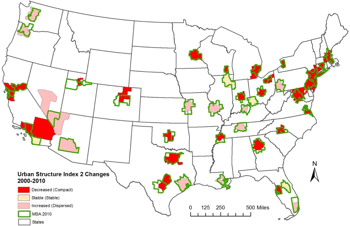
Changes of urban structure index 2 (2000 to 2010).

The Influence of Urban Structure on Commuting

Urban structures are thought to exert influence on commuting patterns (Bento et al. 2005; Clark and Kuijpers 1994). In our study, we hypothesize that the decentralized job density nodes regarding the distribution of residential workers in an MSA will lead to less commuting time. In previous sections, we construct urban structure index 1 and urban structure index 2 to quantify urban structures. For this section, we explore how urban structures affect commuting times in terms of commuting modes: private cars and public transit. The reason we choose these two modes is that workers commuting by these two modes take up a large amount of total commuters. In 2000, the percentage of commuters to work by private cars is 88.61 percent. In 2010, the percentage tapers off to 87.43 percent, indicating still a large amount of commuters commute by private cars. In light of public transits, though the percentages of commuters are not high in 2000 (7.10 percent) and 2010 (8.43 percent), compared to other transportation modes, such as bicycle, motorcycle, or taxicab, public transits are nonnegligible modes for commuters, especially for mega MSAs such as Boston and New York. In 2010, the percentage of public transit commuters account for 11.36 percent and 30.40 percent for Boston and New York, respectively. In addition to urban structure indexes, the number of commuters is considered as an effective factor that influences commuting times. As the number of commuters increases, it brings more traffic onto highways and local expressways. Traffic congestion has the potential to increase commuting times. Considering the large magnitude of the number of commuters, we take its natural logarithmic transformation to reduce the marginal effect. The statistical results are summarized in Table 4.

Table 4.

Impact of Urban Structure on Commuting Time.

	Commuting Time/ΔCommuting Time
Mean Commuting Time	Total	p Value	Private	p Value	Public	p Value
2000 (Forty-six MSAs)
Intercept	−17.86	.00**	−9.62	.08	18.27	0.00***
Log(commuters)	3.27	.00***	2.63	.00***	2.19	0.00***
Urban structure index 1	−4.61	.04*	−3.87	.08	−0.36	0.95
Urban structure index 2	−0.12	.95	0.20	.93	4.81	0.29
Adjusted R ²	.64		.47		.39
2010 (Forty-eight MSAs)
Intercept	−22.40	.00***	−12.40	.05*	22.05	0.00***
Log(commuters)	3.47	.00***	2.70	.00***	1.67	0.00***
Urban structure index 1	−7.33	.01*	−6.26	.02*	1.5	0.82
Urban structure index 2	3.96	.05*	4.14	.03*	8.27	0.07
Adjusted R ²	.67		.57		.33
2000 to 2010 (Forty-two MSAs)
Intercept	−0.89	.06	−0.88	.05*	0.50	0.53
ΔUrban structure index 1	−0.05	.00**	−0.04	.00**	−0.01	0.67
ΔUrban structure index 2	−0.01	.57	−0.01	.70	−0.02	0.65
Adjusted R ²	.26		.20		.01

Note: MSAs = metropolitan statistical areas.

*Indicates .05 level.

**Indicates .01 level.

***Indicates .001 level.

In 2000, a larger number of commuters are associated with longer commuting times. Urban structure index 1, representing how high job density nodes decentralize with regard to residential workers, is statistically negatively associated with commuting time regardless of the mode. This suggests that more decentralization of high job density nodes compared with the distribution of residential workers is related to less commuting time. This result corresponds with the “co-location” hypothesis, which proposes that employment decentralization comes along naturally with firms locating where employees reside (Downs 2000; Gordon, Richardson, and Jun 1991; Lowry 1988), and eventually it would lead to shortened commuting times. The urban structure index 2, representing a decentralization of moderate job density nodes with reference to residential workers, has insignificant impact on commuting times. In other words, the number of commuters who commute to moderate job density nodes accounts for a small portion of commuters as a whole. Thus, the corresponding commuting flows only take up a minor share, which are not captured by the urban structure index 2, and lead to the insignificant relationship between the urban structure index 2 and the commuting times, in both private cars and public transit.

In 2010, similar to 2000, a larger number of commuters are associated with longer total commuting times. A higher urban structure index 1 leads to shorter total commuting times, while a higher urban structure index 2 leads to longer total commuting times. Unlike in 2000, commuting times differ by modes of transportation. Private cars negatively relate with the urban structure index 1 but positively relate with the urban structure index 2, while public transit is barely associated with either urban structure index. So, the expanded distribution of high job density nodes regarding the distribution of residential workers leads to shorter commuting times when using private cars, while the more decentralized moderate job density nodes induce longer commuting times with private cars. Decentralization of high or moderate job density nodes has insignificant effect on commuting times in public transit. Our explanation is as follows: (1) for urban structure index 1, it represents spread levels of high job density nodes compared with the distribution of residential workers, which support substantial number of jobs and appeal to substantial number of commuters. More distributed high job density nodes mean more opportunities for workers living close to them, and thus shorten both total commuting times and commuting times of private cars, in this case, where 87.43 percent of the total number of commuters in 2010 are private car users; (2) for the urban structure index 2, it represents spread levels of moderate job density nodes where the number of jobs or job opportunities is less than the high job density nodes. Moderate job density nodes are not big enough to attract workers to live near them. Thus, commuters working at moderate job density nodes do not take advantage of decentralized job opportunities by locating their houses far away from their workplaces. As a result, the decentralized moderate job density nodes lead to longer total commuting times and the commuting times of private cars. In terms of public transit, existing routes and public transport facilities, such as bus, railway, or subway stations, are lagged when compared with changes in urban structures. Hence, urban structures have insignificant effect on public transit commuting times.

To further explore in a temporal perspective, we analyze how the changes of urban structures affect commuting times. Since MSAs’ boundaries alter remarkably from 2000 to 2010, new incorporated counties of an expanded MSA might bring in commuters, or removed counties from a shrunken MSA might take away commuters. As such, we exclude a predictor: changes of number of commuters. Since the urban structure index 1 and urban structure index 2 are not subject to the MSA’s size, changes of these two indexes illustrate variations of urban structures that are examined ( Table 4). The changes of the urban structure index 1 are negatively associated with the changes of total commuting times, which is consistent with the results for 2000 and 2010. When it comes to modes, only the private mode is significantly associated with changes in commuting times.

Discussion and Conclusions

Two urban structure indexes: urban structure index 1, representing relationship between distributions of high job density nodes and residential workers, and urban structure index 2, representing the relationship between the decentralization of moderate job density nodes and the residential workers, are constructed to quantify urban structures. We find that the decentralization of high job density nodes leads to less total commuting times in both 2000 and 2010, while more decentralized moderate job density nodes compared with the distribution of residential workers lead to longer total commuting times in 2010. This finding can be explained in terms of relocation of jobs and residential workers. Along with the decentralization high job density nodes, jobs gradually migrate to subcenters. Meanwhile, a proper supply of houses, those with reasonable prices or rents, a provision of corresponding service facilities, and establishments of comprehensive communities, constructed together with high job density nodes, encourages willing and capable people to locate close to where they work. Gradually, the expanded distribution of high job density nodes brings workers and jobs closer, reduces commuting time, and potentially reduces traffic congestion, alleviates air pollution, and energy costs. Our finding is consistent with the previous research by Buliung and Kanaroglou (2006), which stated directing urban growth toward suburb activity centers helps reduce weekday travel, and research by Modarres (2011), concluding that the grown subcenters have witnessed shorter commuting times for their residents.

In terms of the decentralization of moderate job density nodes, we find it has insignificant effect on total commuting time in 2000 but is positively associated with total commuting time in 2010. This finding is consistent with the study of Yang et al. (2012), in which they suggested that more decentralization of moderate population density nodes would result in longer commuting times. As for the insignificant effect on commuting times in 2000, the possible explanation is moderate job density nodes do not account for a large proportion of jobs and thus attract a small proportion of commuters. The commuting time by commuters to moderate job density nodes does not contribute too much to the total commuting time.

When we consider commuting modes, commuting time differs by modes. For private cars, more expanded distribution of high job density nodes compared with the distribution of residential workers is associated with shorter commuting times, while more decentralization of moderate job density nodes with regard to the distribution of residences is significantly associated with longer commuting times in 2010. For public transit, the expanded distribution of high or moderate job density nodes with the distribution of residences has insignificant effect.

Besides the findings above, we recognize additional insights. Different from the trend of decentralization, several MSAs become more compact in terms of job and residential distribution, such as the Boston, Philadelphia, New York, Washington, and Chicago MSAs. For example, in Boston, more jobs concentrate in urban cores in 2010 than in 2000, which is exemplified by the changes of job densities as the distance from the CBD increases (Figure 11).

Figure 11.

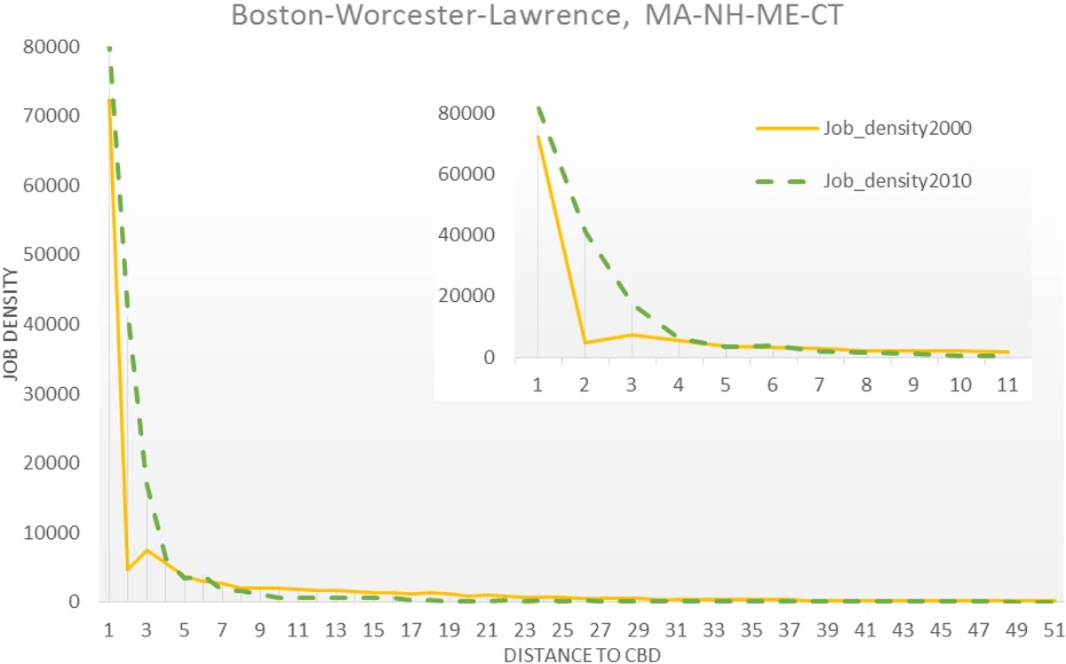
Changes of job densities for Boston MSA.

When analyzing urban structures and how changes of urban structures affect commuting time, previous studies applied the same referential MSA boundaries for different years (Arribas-Bel and Sanz-Gracia 2014; Yang 2008, 2005). MSA boundaries, however, change significantly due to the changes of commuting flows. Using the same boundaries might conceal the actual relationships between urban structures and commuting patterns. Thus, adapting appropriate MSA boundaries for corresponding years may unveil how urban structures affect commuting times more accurately.

Our studies have limitations. First, we only focus on how urban structures affect commuting times temporally rather than emphasizing deriving factors, such as, social and economic factors, or policies. Second, our method to classify high job density nodes and moderate job density nodes needs a solid justification. Although this method is applicable to large MSAs, it has a limitation toward small or some moderate MSAs, because they do not have census tracts with job densities higher than tenfold average job densities in their MSAs. Last, SDEs are sensitive to spatial distribution of input points and polygons. One or two scattered high or moderate job density nodes would enlarge ellipses significantly, and hence, increase urban structure indexes significantly. For example, there are two MSAs: A and B. They have same number of high job density nodes. For A, all high job density nodes are concentrated in urban cores, while for B, most of the high job density nodes are located at urban cores, but also with scattered nodes (Figure 12). The SDE for B is much larger than A, although the scattered high job density nodes might exert a limited effect on commuting times within B.

Figure 12.

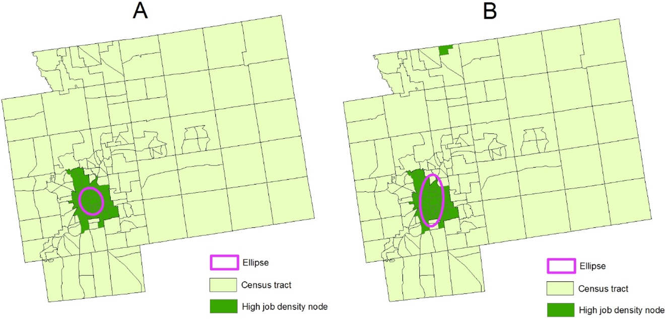
Ellipses for A and B.

Changes of urban forms have been studied through delineating decentralized population and employment since suburbanization emerged (Baumont, Ertur, and Gallo 2004; Craig and Ng 2001; McDonald and McMillen 1990). Since then, many works have explored the impact of urban structures on commuting times but conclusions vary (Cervero and Wu 1997; Gordon, Kumar, and Richardson 1989; Modarres 2011; Schwane, Dieleman, and Dijst 2004; Sultana 2000; Sultana and Weber 2007). We analyze urban structures through exploring the relationships between locations of jobs and housing, which is crucial in understanding the influence of urban structures on urban commuting (Horner 2004). We find that MSAs have different levels of job decentralization with reference to the distribution of residential workers and exert different degrees of impact on commuting times. We show that urban structures affect commuting times in a complex way: the more expanded distribution of high job density nodes with reference to the distribution of residential workers results in shorter commuting times, while the decentralization of moderate job density nodes compared with residential workers leads to longer commuting times. In acknowledging the complex effect of urban structures on commuting times, it is beneficial to encourage and direct the configuration of jobs and residences to form high job density nodes and to achieve an effective distribution of high job density nodes regarding the distribution of residences. Policies, supporting provisions for reasonable housing, employment opportunities, amiable communities, and living amenities, are critical to attract people to work locally and thus decrease cross-zonal commutes and overall commuting time.

Footnotes

Declaration of Conflicting Interests

The author(s) declared no potential conflicts of interest with respect to the research, authorship, and/or publication of this article.

Funding

The author(s) received no financial support for the research, authorship, and/or publication of this article.

References

Aguilera

Mignot

. 2004. “Urban Sprawl, Polycentrism and Commuting. A Comparison of Seven French Urban Areas.” Urban Public Economics Review 1:93–114.

Alonso

William

. 1964. Location and Land Use: Towards a General Theory of Rent. Cambridge, MA: Harvard University Press.

Arribas-Bel

Sanz-Gracia

. 2014. “The Validity of the Monocentric City Model in a Polycentric Age: US Metropolitan Areas in 1990, 2000 and 2010.” Urban Geography 35:980–97.

Batty

2001. “Polynucleated Urban Landscapes.” Urban Studies 38:635–55.

Baumont

Ertur

Gallo

. 2004. “Spatial Analysis of Employment and Population Density: The Case of the Agglomeration of Dijon 1999.” Geographical Analysis 36:146–76.

Bento

A. M.

Cropper

M. L.

Mobarak

A. M.

Vinha

. 2005. “The Effects of Urban Spatial Structure on Travel Demand in the United States.” Review of Economics and Statistics 87:466–78.

Blumenberg

Manville

. 2004. “Beyond the Spatial Mismatch: Welfare Recipients and Transportation Policy.” CPL bibliography 19 (2): 182–205.

Bogart

W. T.

Ferry

W. C.

. 1999. “Employment Centers in Greater Cleveland: Evidence of Evolution in a Formerly Monocentric City.” Urban Studies 36:2099–110.

Boiteux-Orain

Guillain

. 2004. Changes in the Intrametropolitan Location of Producer Services in Île-de-France (1978-1997): Do Information Technologies Promote a More Dispersed Spatial Pattern?” Urban Geography 25:550–78.

10.

Buliung

R. N.

Kanaroglou

P. S.

. 2006. “Urban Form and Household Activity-travel Behavior.” Growth and Change 37:172–99.

11.

Cervero

1996. “Jobs-housing Balance Revisited: Trends and Impacts in the San Francisco Bay Area.” Journal of the American Planning Association 62:492–511.

12.

Cervero

K. L.

. 1997. “Polycentrism, Commuting, and Residential Location in the San Francisco Bay Area.” Environment and Planning A 29:865–86.

13.

Cervero

K. L.

. 1998. “Sub-centering and Commuting: Evidence from the San Francisco Bay Area, 1980–90.” Urban Studies 35:1059–76.

14.

Chowdhury

T. A.

Scott

D. M.

Kanaroglou

P. S.

. 2013. “Urban Form and Commuting Efficiency: A Comparative Analysis Across Time and Space.” Urban Studies 50:191–207.

15.

Clark

W. A.

Kuijpers-Linde

. 1994. “Commuting in Restructuring Urban Regions.” Urban Studies 31:465–83.

16.

Coevering

Schwanen

. 2006. “Re-evaluating the Impact of Urban Form on Travel Patterns in Europe and North-America.” Transport Policy 13:229–39.

17.

Crane

2007. “Is There a Quiet Revolution in Women’s Travel? Revisiting the Gender Gap in Commuting.” Journal of the American Planning Association 73:298–316.

18.

Craig

S. G.

P. T.

. 2001. “Using Quantile Smoothing Splines to Identify Employment Subcenters in a Multicentric Urban Area.” Journal of Urban Economics 49:100–20.

19.

Dieleman

F. M.

Faludi

. 1998. “Polynucleated Metropolitan Regions in Northwest Europe: Theme of the Special Issue.” European Planning Studies 6:365–77.

20.

Downs

2000. Stuck in Traffic: Coping with Peak-hour Traffic Congestion. Washington, DC: Brookings Institution Press.

21.

Ewing

Pendall

Chen

. 2003. “Measuring Sprawl and Its Transportation Impacts.” Transportation Research Record: Journal of the Transportation Research Board 1831:175–83.

22.

Frank

Bradley

Kavage

Chapman

Lawton

T. K.

. 2008. “Urban Form, Travel Time, and Cost Relationships with Tour Complexity and Mode Choice.” Transportation 35:37–54.

23.

Fuji

Tadashi

Hartshorn

T. A.

. 1995. “The Changing Metropolitan Structure of Atlanta, Georgia: Locations of Functions and Regional Structure in a Multinucleated Urban Area.” Urban Geography 16:680–707.

24.

Galster

Hanson

Ratcliffe

M. R.

Wolman

Coleman

Freihage

. 2001. “Wrestling Sprawl to the Ground: Defining and Measuring an Elusive Concept.” Housing Policy Debate 12:681–717.

25.

Garreau

Joel

. 1991. Edge City: Life on the New Frontier. New York: Doubleday.

26.

Garcia-López

M. À.

Muñiz

. 2010. “Employment Decentralization: Polycentricity or Scatteration? The Case of Barcelona.” Urban Studies 47:3035–56.

27.

Giuliano

Small

K. A.

. 1991. “Sub-centers in the Los Angeles Region.” Regional Science and Urban Economics 21:163–82.

28.

Giuliano

Small

K. A.

. 1993. “Is the Journey to Work Explained by Urban Structure?” Urban Studies 30:1485–500.

29.

Giuliano

Genevieve

Redfearn

Christian

Agarwal

Ajay

Chen

Zhuang

Duan

. 2007. “Employment Concentrations in Los Angeles, 1980–2000.” Environment and Planning A 39:2935–57.

30.

Gordon

Kumar

Richardson

H. W.

. 1989. “Congestion, Changing Metropolitan Structure, and City Size in the United States.” International Regional Science Review 12:45–56.

31.

Gordon

Richardson

H. W.

. 1996. “Beyond Polycentricity: The Dispersed Metropolis, Los Angeles, 1970-1990.” Journal of the American Planning Association 62:289–95.

32.

Gordon

Richardson

H. W.

Jun

M. J.

. 1991. “The Commuting Paradox Evidence from the Top Twenty.” Journal of the American Planning Association 57:416–20.

33.

Gordon

Richardson

H. W.

Wong

H. L.

. 1986. “The Distribution of Population and Employment in a Polycentric City: The Case of Los Angeles.” Environment and Planning A 18:161–73.

34.

Greene

D. L.

1980. “Recent Trends in Urban Spatial Structure.” Growth and Change 11:29–40.

35.

Handy

1996. “Urban Form and Pedestrian Choices: Study of Austin Neighborhoods.” Transportation Research Record: Journal of the Transportation Research Board 1552:135–44.

36.

Hajrasouliha

A. H.

Hamidi

. 2017. “The Typology of the American Metropolis: Monocentricity, Polycentricity, or Generalized Dispersion?” Urban Geography 38:420–44.

37.

Horner

M. W.

2004. “Spatial Dimensions of Urban Commuting: A Review of Major Issues and Their Implications for Future Geographic Research.” The Professional Geographer 56:160–73.

38.

Horner

M. W.

2007. “A Multi-scale Analysis of Urban Form and Commuting Change in a Small Metropolitan Area (1990–2000).” The Annals of Regional Science 41:315–32.

39.

Horner

M. W.

Mefford

J. N.

. 2007. “Investigating Urban Spatial Mismatch Using Job–housing Indicators to Model Home–Work Separation.” Environment and Planning A 39:1420–40.

40.

Hoyt

1941. “Forces of Urban Centralization and Decentralization.” American Journal of Sociology 46:843–52.

41.

Wang

. 2016. “Temporal Trends of Intraurban Commuting in Baton Rouge, 1990–2010.” Annals of the American Association of Geographers 106:470–79.

42.

Wang

Wilmot

C. G.

. 2016. “Commuting Variability by Wage Groups in Baton Rouge, 1990–2010.” Papers in Applied Geography 3:14–29.

43.

Ibipo

J. A.

1995. “Racial Differences in the Commuting Behavior of Women in Buffalo, 1980-1990.” Urban Geography 16:23–45.

44.

Kawase

2004. “Changing Gender Differences in Commuting in the Tokyo Metropolitan Suburbs.” GeoJournal 61:247–53.

45.

Kim

Sang

Ban

. 2014. “Exploring Job Centers by Accessibility Using Fuzzy Set Approach: The Case Study of the Columbus MSA.” GeoJournal 79:209–22.

46.

Kim

Sang

Chun

Lee

. 2012. “Exploring Urban Commuting Imbalance by Jobs and Gender.” Applied Geography 32:532–45.

47.

Kloosterman

R. C.

Musterd

. 2001. “The Polycentric Urban Region: Towards a Research Agenda.” Urban Studies 38:623–34.

48.

Kwan

M. P.

Kotsev

. 2015. “Gender Differences in Commute Time and Accessibility in Sofia, Bulgaria: A Study Using 3D Geovisualisation.” The Geographical Journal 181:83–96.

49.

Lang

2003. Edgeless Cities: Exploring the Elusive Metropolis. Washington, DC: Brookings Institution Press.

50.

2010. “Changing Residential and Employment Locations and Patterns of Commute under Hyper Growth: The Case of Guangzhou, China.” Urban Studies 47:1643–61.

51.

Lowry

1988. “Planning for Urban Sprawl.” Transportation Research Board Special Report 220:275–312.

52.

K. R.

Banister

. 2007. “Urban Spatial Change and Excess Commuting.” Environment and Planning A 39:630–46.

53.

Mauch

Taylor

. 1997. “Gender, Race, and Travel Behavior: Analysis of Household-serving Travel and Commuting in San Francisco Bay Area.” Transportation Research Record: Journal of the Transportation Research Board 1607:147–53.

54.

McDonald

J. F.

1987. “The Identification of Urban Employment Subcenters.” Journal of Urban Economics 21:242–58.

55.

McDonald

J. F.

McMillen

D. P.

. 1990. “Employment Subcenters and Land Values in a Polycentric Urban Area: The Case of Chicago.” Environment and Planning A 22:1561–74.

56.

McLafferty

1997. “Gender, Race, and the Determinants of Commuting: New York in 1990.” Urban Geography 18:192–212.

57.

McMillen

D. P.

2001. “Nonparametric Employment Sub-center Identification.” Journal of Urban Economics 50:448–73.

58.

McMillen

D. P.

McDonald

J. F.

. 1997. “A Nonparametric Analysis of Employment Density in a Polycentric City.” Journal of Regional Science 37:591–612.

59.

Melo

P. C.

Graham

D. J.

Noland

R. B.

. 2012. “The Effect of Labour Market Spatial Structure on Commuting in England and Wales.” Journal of Economic Geography 12 (3): 717–37.

60.

Mills

E. S.

1972. Studies in the Structure of the Urban Economy. Baltimore, MD: The John Hopkins Press.

61.

Mitchell

2005. The ESRI Guide to GIS Analysis: Spatial Measurements and Statistics. Redlands, CA: ESRI Press.

62.

Modarres

2011. “Polycentricity, Commuting Pattern, Urban Form: The Case of Southern California.” International Journal of Urban and Regional Research 35:1193–211.

63.

Murphy

2009. “Excess Commuting and Modal Choice.” Transportation Research Part A: Policy and Practice 43:735–43.

64.

Muth

Richard F.

1969. Cities and Housing: The Spatial Pattern of Urban Residential Land Use. Chicago, IL: University of Chicago Press.

65.

Niedzielski

M. A.

Eric Boschmann

. 2014. “Travel Time and Distance as Relative Accessibility in the Journey to Work.” Annals of the Association of American Geographers 104:1156–82.

66.

Office of Management and Budget. 2010. “2010 Standards for Delineating Metropolitan and Micropolitan Statistical Areas.” Federal Register 75:37246–52.

67.

O’Kelly

M. E.

Niedzielski

M. A.

Gleeson

. 2012. “Spatial Interaction Models from Irish Commuting Data: Variations in Trip Length by Occupation and Gender.” Journal of Geographical Systems 14:357–87.

68.

Parr

2004. “The Polycentric Urban Region: A Closer Inspection.” Regional Studies 38:231–40.

69.

Sang

O’Kelly

Kwan

M. P.

. 2011. “Examining Commuting Patterns: Results from a Journey-to-work Model Disaggregated by Gender and Occupation.” Urban Studies 48:891–909.

70.

Schlossberg

Greene

Phillips

P. P.

Johnson

Parker

. 2006. “School Trips: Effects of Urban Form and Distance on Travel Mode.” Journal of the American Planning Association 72:337–46.

71.

Schwanen

Dieleman

F. M.

Dijst

. 2004. “The Impact of Metropolitan Structure on Commute Behavior in the Netherlands: A Multilevel Approach.” Growth and Change 35:304–33.

72.

Scott

L. M.

Janikas

M. V.

. 2010. “Spatial Statistics in ArcGIS.” Handbook of Applied Spatial Analysis 27–41. Accessed August 20, 2017. https://link-springer-com-443.web.bisu.edu.cn/chapter/10.1007%2F978-3-642-03647-7_2?LI=true

73.

Sermons

M. W.

Koppelman

F. S.

. 2001. “Representing the Differences between Female and Male Commute Behavior in Residential Location Choice Models.” Journal of Transport Geography 9:101–10.

74.

Shearmur

Coffey

Dube

Barbonne

. 2007. “Intrametropolitan Employment Structure: Polycentricity, Scatteration, Dispersal and Chaos in Toronto, Montreal and Vancouver, 1996-2001.” Urban Studies 44:1713–38.

75.

Small

K. A.

Song

. 1994. “Population and Employment Densities: Structure and Change.” Journal of urban economics 36 (3): 292–313.

76.

Sohn

2005. “Are Commuting Patterns a Good Indicator of Urban Spatial Structure?” Journal of Transport Geography 13:306–17.

77.

Sultana

2000. “Some Effects of Employment Centers on Commuting Times in the Atlanta Metropolitan Area, 1990.” Southeastern Geographer 40 (2): 225–233.

78.

Sultana

2002. “Job/housing Imbalance and Commuting Time in the Atlanta Metropolitan Area: Exploration of Causes of Longer Commuting Time.” Urban Geography 23:728–49.

79.

Sultana

Weber

. 2007. “Journey- to- Work Patterns in the Age of Sprawl: Evidence from Two Midsize Southern Metropolitan Areas.” The Professional Geographer 59:193–208.

80.

Vandersmissen

M. H.

Villeneuve

Thériault

. 2003. “Analyzing Changes in Urban Form and Commuting Time.” The Professional Geographer 55:446–63.

81.

Veneri

2010. “Urban Polycentricity and the Costs of Commuting: Evidence from Italian Metropolitan Areas.” Growth and Change 41:403–29.

82.

Wachs

Taylor

B. D.

Levine

Ong

. 1993. “The Changing Commute: A Case-study of the Jobs–housing Relationship over Time.” Urban Studies 30:1711–29.

83.

Waddell

1992. “A Multinomial Logit Model of Race and Urban Structure.” Urban Geography 13:127–41.

84.

Wang

2000. “Modeling Commuting Patterns in Chicago in a GIS Environment: A Job Accessibility Perspective.” The Professional Geographer 52:120–33.

85.

Wang

Chai

. 2009. “The Jobs–housing Relationship and Commuting in Beijing, China: The Legacy of Danwei.” Journal of Transport Geography 17:30–38.

86.

Wang

Song

. 2011. “From “Spatial Bond” to “Spatial Mismatch”: An Assessment of Changing Jobs–Housing Relationship in Beijing.” Habitat International 35:398–409.

87.

Yang

2005. “Commuting Impacts of Spatial Decentralization: A Comparison of Atlanta and Boston.” Journal of Regional Analysis and Policy 35:69–78.

88.

Yang

2008. “Policy Implications of Excess Commuting: Examining the Impacts of Changes in US Metropolitan Spatial Structure.” Urban Studies 45:391–405.

89.

Yang

French

Holt

Zhang

. 2012. “Measuring the Structure of US Metropolitan Areas, 1970–2000: Spatial Statistical Metrics and an Application to Commuting Behavior.” Journal of the American Planning Association 78:197–209.

90.

Zegras

2004. “Influence of Land Use on Travel Behavior in Santiago, Chile.” Transportation Research Record: Journal of the Transportation Research Board 1898:175–82.

91.

Zhang

2004. “The Role of Land Use in Travel Mode Choice: Evidence from Boston and Hong Kong.” Journal of the American Planning Association 70:344–60.