New Approach to Economic Convergence in the EU: A Multilevel Analysis from the Spatial Effects Perspective

Abstract

The β-convergence model is based on the neoclassical framework in which the spatial level of analysis is not relevant. These levels will result in decreasing returns. However, local processes of agglomeration, spillover effects, or other forces could operate differently depending on the level of spatial disaggregation. The primary objective of this article is to observe whether different local, regional, and national convergence behaviors are possible in the European Union (EU). To capture the differences among spatial scales, a multilevel and spatial effects extension of the Solow–Swan theoretical growth model is proposed. The estimations of this model are made using consistent information from Eurostat and Cambridge Econometrics for the period of 2000–2014. A multilevel spatial Durbin model estimator is applied to evaluate the spatial interactions of the regions. The results indicate that a general process of convergence in the EU coexists with intranational processes of divergence, highlighting the relevance of the spatial level of analysis. A final analysis of the impact of the economic crisis over the general behavior has been included verifying that the economic crisis strongly reinforce the weakness of the EU convergence.

Keywords

multilevel models spatial Durbin model European Union

Introduction

Since its inception, the European Union (EU) has been conceptualized both to create economic integration and to develop social and economic cohesion among European nations and regions. Consequently, the study of the evolution of territorial disparities and economic convergence has always been a core issue in the EU, explaining the large number of β-convergence analyses for all of Europe and specific European areas or countries. The improvements in $β$ -convergence estimations developed in the international literature during the last three decades have been widely applied to EU data. Nevertheless, the results for this continent depend heavily on the period of analysis, data sets, methodological approaches, or variables considered, leading to incoherent conclusions among the different analyses about the speed or even existence of convergence within EU regions (see the meta-analysis of Abreu, De Groot, and Florax 2005). However, despite the large number of papers on the EU case, there is still room for improvement in the $β$ -convergence estimation, given the specific complexity of this area with its different institutions operating at different spatial levels and with different local and national dynamics and considering the relevance of the recent economic crisis that has specifically affected the weaker economies in Europe.

In this article, a $β$ -convergence analysis for the EU that uses data from 2000 to 2014 is presented. This allows us to observe the recent growth and convergence dynamics, especially taking into account the important dimension of the recent great international economic recession. Apart from the recent data used, the main contribution of this article is to reflect the real spatial and institutional complexity of the EU using a multilevel model with spatial effects, defining a new empirical approach based on an extension of the Solow–Swan theoretical growth model. With this approach, and by using consistent information from Eurostat and Cambridge Econometrics, it is possible to observe how the conclusions vary from the most disaggregated level (in which agglomeration economies and other local economic forces and policies work) to the most aggregated level (in which the macroeconomic dynamics and national and international policies operate).

Since the seminal papers of Abramovitz (1986) and Baumol (1986), $β$ -convergence analysis has continuously advanced by incorporating relevant improvements in the estimations (for a sample of the evolution of the techniques applied to study $β$ -convergence see, among others, Islam 2003; Magrini 2004; Alexiadis 2013). One of the primary and more recent improvements comes with the development of spatial econometrics (Anselin 1988; Anselin and Florax 1995; Anselin and Rey 1997). In these models, regions interact with each other, and a proper estimation of any spatial analysis, including convergence studies, requires incorporating the interactions between spatial units. Ertur and Koch (2007) propose a theoretical model with spatial interactions by suggesting a spatial Durbin model (SDM) as a suitable empirical framework. Battisti and Vaio (2008), Mella-Marquez and Chasco-Yrigoyen (2006), and Ramajo et al. (2008) use variations of this approach in some of the more recent studies on EU regional convergence. Additionally, Durlauf and Johnson (1995); Durlauf (2000); Postiglione, Benedetti, and Lafratta (2010); Postiglione, Andreano, and Benedetti (2013); and Castellacci, Los, and de Vries (2014) focus on the presence of a heterogeneous process of convergence in groups with the outcome being a set of “convergence clubs.” They suggest that the speed of convergence and the steady state of each territory depend on the group to which it belongs. Standard measurements of convergence, namely, with only one convergence coefficient, would fail to identify this type of heterogeneity. This line of research was also successfully applied in studies of Europe by authors such as Cheshire and Carbonaro (1996), Bartkowska and Riedl (2012), and Monfort, Cuestas, and Ordonez (2013). All these applications for the European case of modern approaches reveal how the initial results that show a moderate, slow convergence need to be nuanced by intense spatial interactions or clustering processes, making the conclusions even more dispersed depending on the technique, the period, or the considered area.

Great attention has been placed on improving the estimation and on including spatial dependence and spatial heterogeneity. This contrasts with the limited attention placed on the relevance of the spatial level of analysis. Under the neoclassical framework, it is assumed that decreasing returns are the theoretical fulfillment of all spatial constructs and all levels of spatial disaggregation; however, urban and regional economic theories as well as the New Economic Geography framework (Krugman 1991; Krugman and Venables 1995; Fujita and Krugman 1995) underline the local dimension of agglomeration economies and other sources of spatial disparities (see Fujita, Krugman, and Venables 2001). In addition, a parallel body of literature, called the modifiable areal unit problem (MAUP), has explored the consequences of aggregating local information within larger regions or changing the groupings of regions (see Gehlke and Biehl 1934; more recently, Openshaw and Taylor 1979; Openshaw 1984). According to this literature, aggregated data could conceal heterogeneous intraregional patterns of behavior. Arbia and Petrarca (2011) study the consequences of the MAUP in general estimations, and Díaz-Dapena, Fernández-Vázquez, and Rubiera-Morollón (2016) study the particular issue of the MAUP in β-convergence estimations.

Based on the potential existence of an MAUP when national or regional data are used and on the underlining local dimension of most spatial effects, the multilevel methodology can be considered a relevant tool in the estimation of economic phenomenon affected by intense spatial heterogeneity or a hierarchical spatial structure (see the examples of Cohen 1998; Elhorst and Zeilstra 2007; Li and Wei 2010; Srholec 2010; Andersson, Hammarstedt, and Hussain 2013; Zeilstra and Elhorst 2014).¹ Despite the growing applications of this empirical approach in other areas of economics, there is scarce empirical evidence of the importance of the spatial scales in convergence studies. To the best of our knowledge, only Chasco and López (2009) for Europe; Díaz-Dapena, Rubiera-Morollón, and Paredes-Araya (2017) for the United States; and Díaz-Dapena, Rubiera-Morollón, Pires, et al. (2017) for Brazil measure the importance of the spatial scales. In all the previous papers, the multilevel approach does not include spatial effects. As was discussed in the previous paragraphs, the absence of spatial integrations is an important limitation in convergence studies. As Ertur and Le Gallo (2009) and Rey and Le Gallo (2009) perfectly explain, individual regions cannot be analyzed as independent observations ignoring the relevance of the interaction between spatial units.

Departing from the Ertur and Koch (2007) economic model, the aim of this article is to incorporate the spatial effects in a multilevel β-convergence model that would allow us to measure the importance and relevance of each scale in a process with heterogeneous behaviors and spatial interactions. This method includes an explicit spatial hierarchy in the empirical specification to identify an integrated process across the EU within a group of independent countries that have individual processes of growth and convergence. Consequently, the proportional contribution by each level could be a measure of an explicit hierarchy in the multilevel model. The model could be used as a starting point from which different variables are added in addition to the effect from bordering regions or countries to measure the spatial spillover effects among the regions/countries. Using the multilevel method, we show both the importance of the hierarchy in the process of convergence in Europe and the spatial interactions among territories.

The advantages of this approach are double. From a technical point of view, several authors (e.g., Ertur and Gallo 2009; Ertur and Koch 2007) emphasize how diversity between regions could be a source of spatial heterogeneity. This heterogeneity could be successfully captured in a multilevel model, which allows us to obtain different estimations for the different levels of the spatial hierarchy.

From the policy makers’ perspective, the importance of each spatial level is crucial to identifying problems of polarization and to informing regional policies. For example, a potential scenario could be a homogeneous process of convergence. This situation would generally imply that the policy maker only has to focus on the possible differences of the steady state at the regional level. A second case is a process of convergence that is mainly driven at an aggregate scale with different steady states. In this case, there are variables beyond the control of the regional level, which determine their steady state and which need to be fixed at an aggregate level. Finally, there is a third process where the convergence at an aggregate scale exists with different steady states and speeds of convergence. This scheme adds the possibility of polarization of some economies to the previous case.

This article is structured as follows. The second section presents the economic model used as the framework. In the third section, the econometric strategy and the multilevel estimation with spatial effects applied to this study are explained. The fourth section presents the empirical application and its results, including a section in which the specific impact of the international economic recession is specifically studied. The fifth section presents the study’s conclusions and a discussion.

Economic Model: β-Convergence Model with Explicit Spatial Interaction

The model of Ertur and Koch (2007) is used as the theoretical basis for the empirical approach; for an extended explanation of this model, see Lacombe and McIntyre (2017) or Elhorst, Piras, and Arbia (2010). The model is an extension of the Solow–Swan model that is used in the majority of the literature on convergence with explicit spatial interactions that represent the interactions highlighted by previous authors such as Rey and Montouri (1999). The model assumes a Cobb–Douglas production function, which depends on the aggregate level of technology, the aggregated level of physical capital and labor:

Y_{i} (t) = A_{i} (t) K_{i}^{α} (t) L_{i}^{1 - α} (t) .

$Y_{i} (t)$ describes production, $K_{i} (t)$ the physical capital, $A_{i} (t)$ the current state of technology, and $L_{i} (t)$ is the relevance of labor. The aggregate level of technology is defined as follows:

A_{i} (t) = Ω (t) k_{i}^{ϕ} (t) \prod_{j \neq i}^{N} A_{j}^{γ w_{i j}} (t) .

The first component represents an exogenous growth over time as in the Solow–Swan model. This component grows at a constant rate $μ$ following as in equation (3):

Ω (t) = Ω (0) e^{μ t} .

The second component of the technology function represents the influence of the rate of capital per worker, $k_{i} (t) = K_{i} (t) / L_{i} (t)$ . This component has a positive effect on technology when $ϕ$ is above 0. As a result, investments in physical capital increase production through the components of cumulative capital and technology. As in Ertur and Koch (2007), the last component is the influence of the technology in the neighboring regions. $w_{i j}$ denotes the connectivity parameters with the rest of the j regions. These parameters are assumed to be nonnegative and the sum of all the connections to region i is equal to 1. This component explicitly represents the spatial interactions through the spatial diffusion of technology also known as spillover effects. This model takes into account that the diffusion of technology across firms does not have to be restricted within the borders of a territory. The degree of spatial interactions is represented by the parameter $γ$ . Under the described assumptions in $w_{i j}$ , the range of this parameter is $0 \leq γ < 1$ .

Taking logarithms, equation (2) can be expressed in its matrix form:

A = Ω + ϕ k + γ W A,

where A is a vector with the logarithms of technology, k is a vector of physical capital per worker in logarithms, whereas W is the spatial weight matrix of the $w_{i j}$ terms. A can be solved when $γ$ is not the inverse of an eigenvalue of W.²

A = {(I - γ W)}^{- 1} Ω + {(I - γ W)}^{- 1} ϕ k .

Taking logarithms in equation (1) and replacing A with equation (5), the production function per worker can be expressed as in equation (6) in its matrix form:

y = Ω + (α + ϕ) k - α γ W k + γ W y,

where y is a vector of the production per worker in logarithms. As in the Solow model, the capital growth is assumed to be a fraction of the production $s_{i} y_{i} (t)$ , labor grows at a constant rate n_i , the physical capital depreciates at a constant rate $δ$ , and technology grows at a constant rate g. So, following this model, the capital per worker in the steady state in logarithms can be expressed as in equation (7):

l n k_{i}^{*} (t) = l n y_{i}^{*} (t) + ln [s_{i} / (n_{i} + g + δ)],

where g is the usual rate of technological growth toward the economy tends to grow in the steady state. Using this information in equation (6), the output per worker in the steady state for an economy i can be solved as in equation (8).

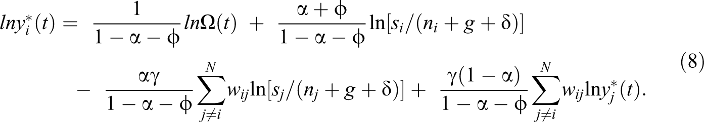
\begin{array}{l} l n y_{i}^{*} (t) = \frac{1}{1 - α - ϕ} l n Ω (t) + \frac{α + ϕ}{1 - α - ϕ} ln [s_{i} / (n_{i} + g + δ)] \\ - \frac{α γ}{1 - α - ϕ} \sum_{j \neq i}^{N} w_{i j} ln [s_{j} / (n_{j} + g + δ)] + \frac{γ (1 - α)}{1 - α - ϕ} \sum_{j \neq i}^{N} w_{i j} ln y_{j}^{*} (t) . \end{array}

As explained in Ertur and Koch (2007), this model has a similar interpretation to the Solow model. The elasticities of the rate of savings are positive, while the depreciation rate of capital and the population growth have the same elasticity as the saving rate in absolute terms but opposite sign.

The rate of savings in the neighbors has a negative sign. Nevertheless, the rate of saving affects the steady state in the neighboring economies. This positive effect through the steady state is more important than the negative part, making the elasticity positive, as explained in Ertur and Koch (2007).

Following Ertur and Koch (2007), the convergence equation can be found as the difference between $l n y_{i} (t) and - l n y_{i} (0)$ . $l n y_{i} (0)$ represents the income per capita in logarithms of an initial period.

l n y_{i} (t) - l n y_{i} (0) = C_{i} - (1 - e^{- λ_{i} t}) l n y_{i} (0) + (1 - e^{- λ_{i} t}) l n y_{i}^{*} (t) .

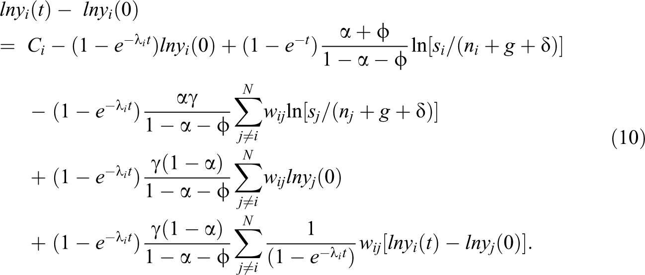
In this equation, C_i represents an exogenous component of the growth equation and $λ$ is the parameter of the speed of convergence. By merging equations (8) and (9), the conditional convergence equation can be expressed as in equation (10).

\begin{array}{l} l n y_{i} (t) - l n y_{i} (0) \\ = C_{i} - (1 - e^{- λ_{i} t}) l n y_{i} (0) + (1 - e^{- t}) \frac{α + ϕ}{1 - α - ϕ} ln [s_{i} / (n_{i} + g + δ)] \\ - (1 - e^{- λ_{i} t}) \frac{α γ}{1 - α - ϕ} \sum_{j \neq i}^{N} w_{i j} ln [s_{j} / (n_{j} + g + δ)] \\ + (1 - e^{- λ_{i} t}) \frac{γ (1 - α)}{1 - α - ϕ} \sum_{j \neq i}^{N} w_{i j} l n y_{j} (0) \\ + (1 - e^{- λ_{i} t}) \frac{γ (1 - α)}{1 - α - ϕ} \sum_{j \neq i}^{N} \frac{1}{(1 - e^{- λ_{i} t})} w_{i j} [l n y_{i} (t) - l n y_{j} (0)] . \end{array}

The assumption of a unique speed of convergence is too strong in the case of economies that are not fully integrated. Several authors have previously noted that each region could have its own steady state (see Canova and Marcet 1995; Islam 1995, 2003; or even Ertur and Koch 2007). From a different point of view, the multilevel approach proposed by Goldstein (1986); Duncan, Jones, and Moon (1998); and Hox (2010) incorporates this feature by focusing on the effect of the hierarchy on a dependent variable. This multilevel approach identifies the relative importance of each level of aggregation. An example of this method is Ballas and Tranmer (2012). They use the UK census to identify the relative importance of area, household, and individual characteristics to variations in happiness. We adapt this hierarchy concept to geographical space, and there is the possibility of the existence of different processes of convergence at different spatial levels.

Econometric Specification

The multilevel model proposed for the convergence equation is shown in equation (11).

y_{i j} = β_{j} x_{i j} + γ z_{i j} + ∊_{i j},

11a

β_{j} = β + v_{j},

11b

E (v_{j}) = 0, var (v_{j}) = V,

11c

V = (\begin{matrix} var (v_{0 j}) & cov (v_{0 j}, v_{1 j}) & \begin{matrix} L & cov (v_{0 j}, v_{k - 1, j}) \end{matrix} \\ cov (v_{0 j}, v_{1 j}) & var (v_{1 j}) & \begin{matrix}  \end{matrix} \\ \begin{matrix} ⋮ \\ cov (v_{0 j}, v_{k - 1, j}) \end{matrix} & \begin{matrix}  \end{matrix} & \begin{matrix} O \\ var (v_{k - 1, j}) \end{matrix} \end{matrix}),

11d

∊_{i j} \sim N (0, σ_{j}^{2}),

11e

where i represents each of the N subnational units or regions while j indices each of the M group of regions or nations. In this specification, the dependent variable ( $y_{i j}$ ) is regressed over a set of k variables ( $x_{i j}$ ) with random coefficients and a set of variables ( $z_{i j}$ ) with no random coefficients. In our case, our variable of interest would have a random slope while the control variables are assumed to have fixed coefficients—see Database section. In the multilevel literature, this type of model is termed a random slope model. The random slope model has a vector ( $β_{j}$ ) of random parameters that differs among countries by the regional variables. $β_{j}$ can be divided into two components, a general or fixed vector β for the entire sample and a random vector (v_j ) that varies among countries. Within v_j the parameters associated with the constant in $x_{i j}$ are called random intercepts $(v_{0 j})$ , while the parameters associated with the effects of other columns in $x_{i j}$ are the random slopes ( $v_{1 j}$ ,…, $v_{k - 1, j}$ ). Matrix V represents the variability in the random parameters through the variances of the random parameters associated with each of the k variables in $x_{i j}$ — $var (v_{0 j}), var (v_{1 j}), \dots, var (v_{k - 1, j})$ —and the covariances between. In addition, $γ$ represents a vector of fixed responses. This model is a general case of the basic estimation of convergence. If there is no variability in the parameters, then we will have the traditional model of convergence for one geographic level. Additionally, robustness to heteroscedasticity is introduced through the specification of group variances of the error ( $σ_{j}^{2}$ ) in the model.

Through this representation, multilevel analysis can represent the correlations between observations that the hierarchy generates. Thus, the result of this type of estimation should help to understand not only the influence of each variable but also the importance of each level of the analysis. According to Hox (2010), in a multilevel problem, there is no proper level for the analysis but all levels are important in their own way.

Using this model, the variability in $β_{j}$ gives important information in our analysis of convergence. Note that this parameter would represent a homogeneous process of convergence for any region and any country and another for each country if we had used a standard linear regression approach. However, here, the convergence parameter has an associated variance of v_j . For example, a negative (positive) value of the coefficient of a specific country would indicate a faster (slower) process of convergence in that country. This is the crucial advantage of these models, and we use this feature to capture the spatial variability behind the convergence in the EU. This type of estimation focuses on an accurate estimate of variability. As a result, the additional orthogonality assumption of a random distribution of this variability allows us to change the focus of the analysis from conventional methodological approaches.

A frequent problem in convergence analysis is the possible bias in the estimation caused by spatial interactions. Different econometric models can be used to capture these interactions (see LeSage and Pace 2009). Depending on the explicit expression of the spatial interaction, there are different econometric strategies. The spatial lag spatial auto regressive (SAR) model assumes a data generating process in which the dependent variable depends on the mean value of the dependent variable in the neighbors. The spatial error model assumes a spatial dependence within the error term. It is also possible to assume that the dependent variable depends on the spatial lag of the independent variables through the “spatial lag of X” model. Finally, when the model includes lags of the dependent and the independent variables, we would have the SDM.

Our results are based on the empirical approach of the SDM. This model has the advantage of being the nesting version of the other three models (see Elhorst 2014). Thus, it avoids the possible weakness in the analysis by choosing one of them. In addition, as explained in LeSage and Pace (2009), this model reduces the omitted variables bias compared to ordinary least squares (OLS), which is an important motivation to use it in empirical research. In addition to the empirical advantages of this model, SDM has been chosen due to the theoretical background. As explained in Economic Model: -Convergence Model with Explicit Spatial Interaction section, our dependent variable is related to spatial lags of both the dependent and the independent variables.

As a result, the spatial dependence of equation (9) is included through an SDM with multilevel effects (for more information about spatial interactions, see Ertur and Koch 2007; Corrado and Fingleton 2012). This type of model includes spatially lagged dependent and independent variables. The estimation strategy is based on a similar method used in the model proposed by Elhorst and Zeilstra (2007) to include spatial dependence in the errors.

In Elhorst and Zeilstra (2007), the authors addressed the endogeneity caused by the temporal dependence of the dependent variable in a multilevel framework with spatially correlated error terms. They applied a method using instrumental variables to obtain consistent estimates. Following this procedure, this article proposes a method consisting of instrumental variables, similar to the two stage least squares (2SLS) method (see Kelejian 1974), to estimate an SDM in a multilevel framework. There is extended literature addressing the use of instrumental variables in the context of spatial dependence, as explained in Anselin (1988). This model is based on López-Bazo, Vayá, and Artís (2004), which includes the spatial lag of the initial output per capita and the dependent variable.

The second problem of this estimation is the common problem of regional heteroscedasticity. The assumption of homoscedastic error terms might create an unreliable inference of the estimators. This problem is addressed using an estimate of a homoscedastic error term for the different groups of the sample.

The econometric strategy—in matrix notation—defines Y as the vector of dependent variables. An X matrix defines the variables with random coefficients. The Z matrix denotes the variables with no random coefficients. Matrix v represents the different random vectors (v_j ) for each group and $∊$ the residuals. The proposed model is defined by equation (12):

Y = X β + Z α + diag (X_{1}, . . ., X_{j}, . . ., X_{M}) v + ∊ .

To represent hierarchy in matrix notation, the influence of variables in X is divided into two components. Vector β represents the common influence of the variables X over Y. The difference in slopes as well as intercepts is obtained by multiplying a block diagonal matrix of X by v. Each block represents the information in X for each of the j group of the hierarchy.

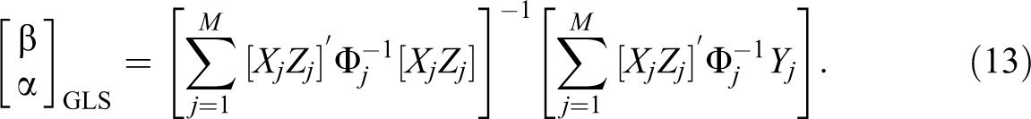
Following Elhorst and Zeilstra (2007), equation (12) can be estimated using the generalized least squares (GLS) estimator. This estimator is defined by equation (13) and is equivalent to the multi-level (ML) estimator when there are no endogenous variables in Z.

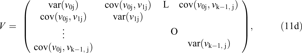
{[\begin{matrix} β \\ α \end{matrix}]}_{GLS} = {[\sum_{j = 1}^{M} {[X_{j} Z_{j}]}^{′} Φ_{j}^{- 1} [X_{j} Z_{j}]]}^{- 1} [\sum_{j = 1}^{M} {[X_{j} Z_{j}]}^{′} Φ_{j}^{- 1} Y_{j}] .

The usual problem of this kind of estimation is estimating the covariance matrix ( $Φ$ ). In multilevel methodology, $Φ$ is the covariance matrix of the term $diag (X_{1}, . . ., X_{j}, . . ., X_{M}) v + ∊$ of equation (12). As a result, this matrix is a block diagonal matrix, where each j block is defined by equation (14):

Φ_{j} = X_{j} V X_{j}^{′} + σ_{j}^{2} I_{j},

where the variability is the sum of the variability in the group residuals— $diag (X_{1}, . . ., X_{M}) v$ and common residuals ( $∊$ ) with M group-homoscedastic variances ( $σ_{j}^{2})$ . As explained above, V is a $k \times k$ matrix with the variance of the intercepts, the k − 1 slopes and the covariances between them (see equation [11d]). For additional information about the computational approach, see Elhorst and Zeilstra (2007) or Frees (2004).

The first problem of this type of estimation is that V and $σ_{j}^{2}$ are unknown. To address this problem, this article applies the Swamy (1970) method. This method applies an asymptotically efficient feasible generalized least squares (FGLS) estimator. In the first step, the model is estimated assuming fixed responses for the X variables that are different for each country, as is Z. The coefficients of this model are used to estimate V according to equation (15).

\hat{V} = \frac{1}{N - 1} \sum_{j = 1}^{M} ({\hat{β}}_{j}^{F} - \frac{1}{M} \sum_{j = 1}^{M} {\hat{β}}_{j}^{F}) {({\hat{β}}_{j}^{F} - \frac{1}{M} \sum_{j = 1}^{M} {\hat{β}}_{j}^{F})}^{′} .

In the last step, this estimation of V allows us to apply the estimator proposed in equations (13) and (14). Group variances are estimated using equation (16), and then, the fixed parameters are estimated again until convergence.

{\hat{σ}}_{j}^{2} = e_{j}^{′} e_{j} / N_{j} .

However, equation (13) might produce biased estimators due to the endogeneity caused by spatial dependence. This problem is addressed through an estimation using instrumental variables. The instrumental variable approach of GLS (G2SLS) has been applied following Amemiya (1985). This estimation applies a multilevel structure in both steps. First, a multilevel model is used to predict the spatial lag of the dependent variable according to a set of instrumental variables. Then, the predicted variable and the other exogenous variables are used to regress the dependent variable. The estimator is defined in equation (17):

{\hat{b}}_{G2SLS} = {(\hat{S^{'}} Φ^{- 1} \hat{S})}^{- 1} \hat{S^{'}} Φ^{- 1} Y where \hat{S} = P {(P^{'} Φ^{- 1} P)}^{- 1} P^{'} Φ^{- 1} S,

where S is a matrix with one or more endogenous variables and P contains the exogenous variables in S and the instrumental variables. The instrumental variables were chosen following Kelejian, Prucha, and Yuzefovich (2004). They are obtained from the linear independent columns of ${X, W X, . . ., W^{q} X, Z, W Z, . . ., W^{q} Z}$ which cannot be found in matrix S. In our SDM scenario, the first three independent columns not available in S are used in the projection matrix of instruments— ${W^{2} X, W^{3} X, W^{4} X}$ . Columns ${X, W X$ } have been discarded because they are part of matrix S in an SDM context. The estimation process in equation (17) is used in the first and last step of the FGLS estimation to obtain a consistent estimation of the parameters.

When the specification has been found, the multilevel method makes it possible to measure the importance of each level in the process of convergence. The relative importance of the groups to the total variability of the dependent variable is estimated using the variance partition coefficient (VPC) as in equation (18):

{VPC}_{j} = \frac{X_{j} V X_{j}^{′}}{X_{j} V X_{j}^{′} + σ_{j}^{2}} .

This percentage is the quotient of the total variability between countries and the total variability. Thus, it represents the importance of the hierarchy. The mean of the VPC can be calculated to obtain a representative measurement for the entire sample.

Application to the EU

Database

Our empirical analysis is carried out with regional level data for the EU. Following Escriba and Murgui (2014), the Cambridge Econometrics database provides homogeneous information on the income for all EU regions in constant 2005 terms. In addition, the Eurostat database provides information on the control variables. We need data that are disaggregated at different levels, from the local to the national. Thus, we need information on the Nomenclature des Unités Territoriales Statistiques-III (NUTS-III) regions, which are the most disaggregated levels that have information on gross domestic product per capita (GDPpc). A total of 1,276 regions from 27 countries are included in the analysis.³ The period of analysis is 2000–2014, which is the longest period available using data at this level of spatial disaggregation.

To view the spatial distribution of wealth, Figure 1 presents the GDPpc in 2000 for the NUTS-III in the EU adjusted using the purchasing power parity (PPP) of the countries. It is clear that the largest levels of GDPpc are concentrated in the central areas of the EU. The spatial concentration of the growth and levels of GDPpc is extremely important, especially when it is mixed with the weak process of convergence described above. Together, these two processes describe a territory with a rich core that other regions find difficult to reach.

Figure 1.

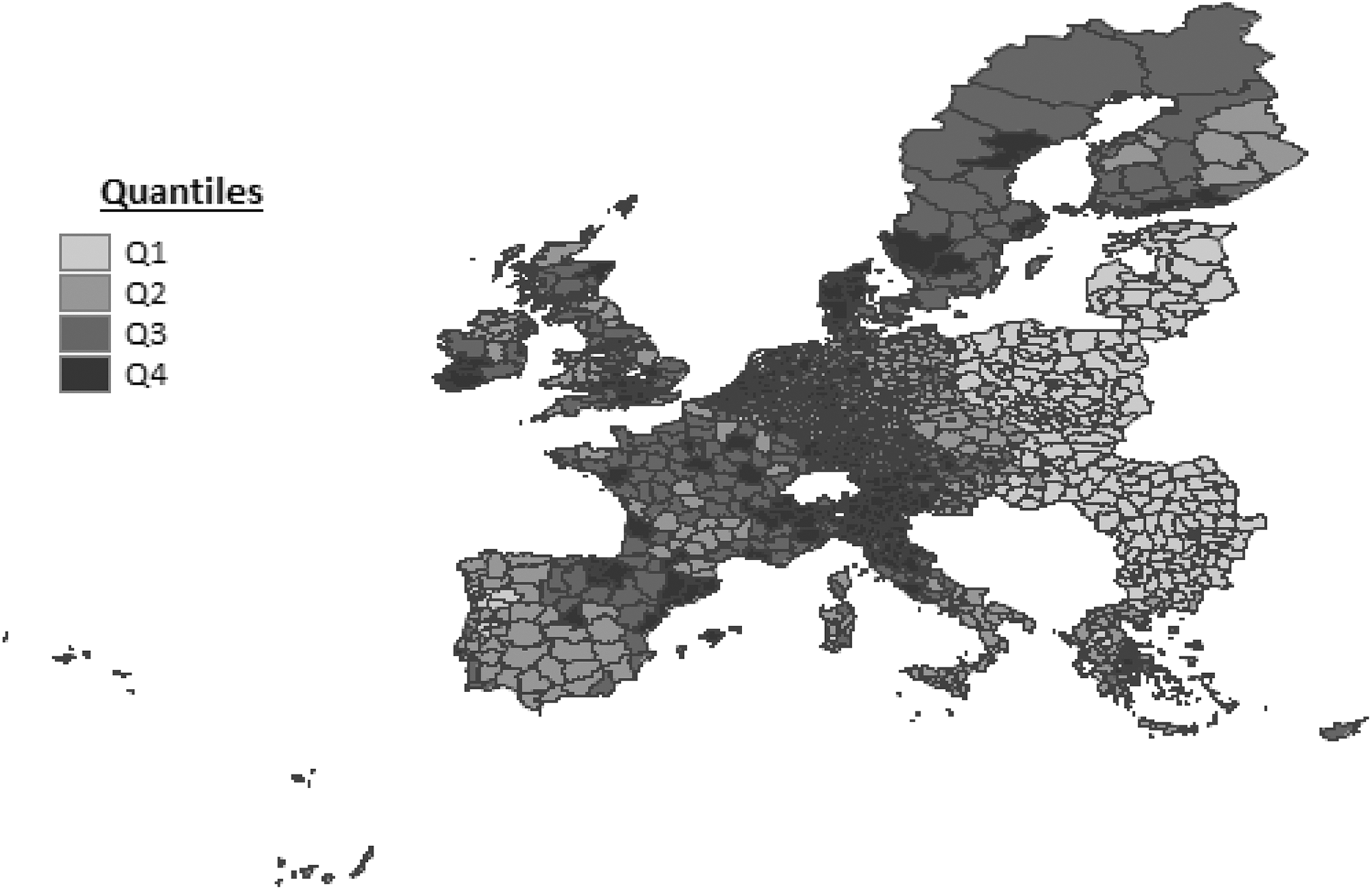
Map of the gross domestic product per capita in PPS^a of the NUTS-III in 2000. ^aPurchased parity standard provided at the country level.

To apply the model proposed in equation (9) to the EU, we need data on the GDPpc in the PPP of each region and information on the main variables that describe the steady state. In addition, multilevel analysis requires information on the country to which each region belongs, whereas the spatial specification requires the geographic position of the centroids. The initial GDPpc (in logarithms) and the constant term are used to build matrix X in equation (12). Table 1 summarizes the data included in the analysis in terms of equation (10) and provides the standard descriptive statistics.

Table 1.

Descriptive Statistics of the Variables.

Variables	Variable	Mean	Standard Deviation	Min.	Max.
Growth of GDPpc in PPS	$L n (y^{2014}) - L n (y^{2000})$	0.147	0.19	−0.334	0.839
GDPpc (€) in PPS in the first period	$y^{2000}$	20,184	10,022	2,636	13,6393
Percentage of population with a level 3–4 of education	h ₁	46.936	15.126	7.3	77.8
Percentage of population with a level 5–8 of education	h ₂	19.843	7.790	3.7	48.9
Gross capital formation as a percentage of GDP	s	21.977	2.707	17.8	29.9
Mean growth of the working population	n	0.625	0.589	−1.154	2.837
R&D expenditures as a percentage of GDP	g	1.732	0.825	0.25	4.13

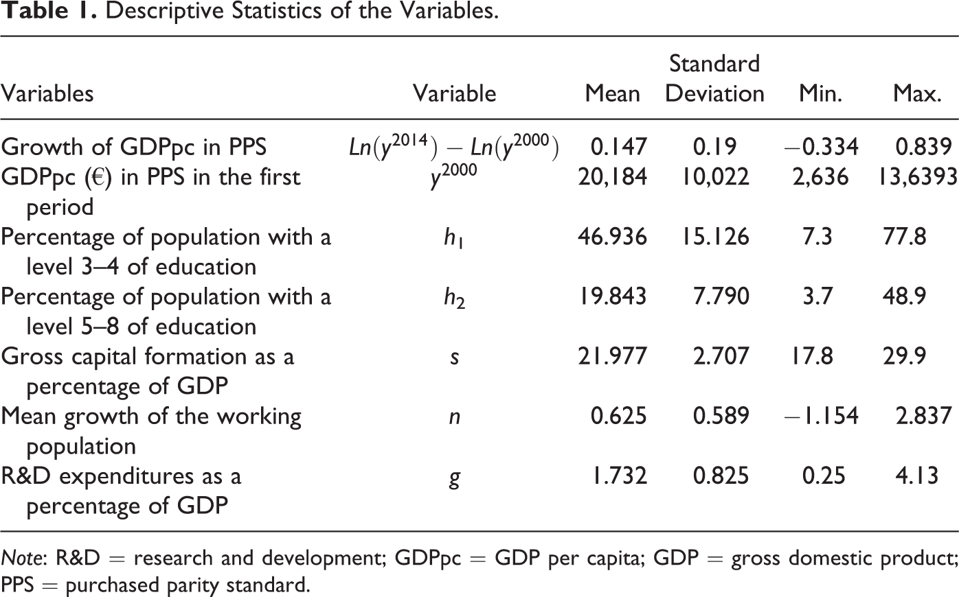
Note: R&D = research and development; GDPpc = GDP per capita; GDP = gross domestic product; PPS = purchased parity standard.

The variables needed to describe the steady state are the rate of savings, the growth in the labor force, the growth in technology, depreciation, and human capital. The rate of investment is the percentage of gross capital formation with respect to GDP. The growth in the labor force is estimated as the growth rate of the working population. The growth in technology is a proxy variable of total research and development (R&D) expenditures as a percentage of total GDP in the country. Depreciation is assumed to be constant and equal to 3 percent. The values of these variables are used to create the coefficient of the Solow’s model, $\frac{s}{n + g + d}$ . The model divides the percentage of gross capital formation with respect to GDP by summing the growth rate of the working population, the rate of R&D expenditures, and the depreciation rate. This coefficient is provided on a national scale. Therefore, their coefficient will be consistent across the entire sample.

Finally, human capital is included with two proxy control variables in order to avoid the bias found in Mankiw, Romer, and Weil (1992). The two variables are the percentage of the population that is from 25- to 64-year-olds in the NUTS-II region with a level 3–4 education (upper secondary and postsecondary nontertiary education) and the percentage with a level 5–8 education (tertiary education).⁴

Control variables are assumed to have fixed parameters in the analysis. Therefore, the control variables $\frac{s}{n + g + d}, h_{1}, and h_{2}$ were included in the Z matrix with the spatial lags. This limitation implies some caution in the interpretation of the results. As shown in equation (10), the rest of the coefficients might also have a variation. Therefore, in case of available information, this estimation could be enhanced by including the indirect effect of heterogeneity on the speed of convergence through the rest of the components. However, our estimation should be able to identify the direct effect of the hierarchy in the convergence process.

Although we could try to estimate a model with random coefficients in all the coefficients, there are different reasons that make this option inadvisable. From an econometric point of view, there should be variability within each group to identify the effect of the hierarchy. This identification becomes even more difficult when all the variables have random parameters. In addition, the number of regions within each country is not homogeneous. Some countries have only a few regions (e.g., Ireland or Latvia). Thus, choosing a complex structure in the hierarchy implies reducing the number countries with a small number of regions. This trade-off becomes even more evident when some variables (R&D or human capital) only have information for NUTSII. Since it is not possible to choose all the variables, this analysis focuses in the variable of interest in order to have the ability to use the multilevel perspective in the biggest sample possible. Even for this case, Luxemburg, Malta, and Cyprus random effects could not be estimated due to the number of NUTS-III in these countries. To avoid extrapolation in the analysis, they were not used in our estimations.

Finally, there is the possible risk of the omission of significant variables. However, the variables of this estimation were chosen according to a well-known theoretical model (Economic Model: -Convergence Model with Explicit Spatial Interaction section). As a result, this possible endogeneity problem is minimized. To reduce this problem, the estimations have also been conducted using additional variables. These variables are the activity rates, densities, and dummy regions with a national capital, internal border, external border, coast, and Eurozone membership.

Results I: The Relevance of the Spatial Scale and Spatial Interactions

Table 2 summarizes all the results obtained using consistent information for the EU from Eurostat and Cambridge Econometrics for 2000–2014. The first and second columns show the robust OLS estimation of unconditional and conditional β-convergence. The conditional model includes the variables as shown in equation (10). Then, the model becomes more complex in order to introduce the hierarchy. The third column presents the multilevel estimation of the unconditional convergence using robust GLS as in equations (13) –(16). The fourth column includes random slopes and intercepts in the conditional β-convergence equation. Finally, the fifth column presents the final complete model with random slopes and intercepts and spatial effects with an SDM specification, as in the Ertur and Koch (2007) model through G2SLS. First, we will briefly discuss the estimations with OLS and the simplest multilevel approaches, which will allow us to enter and extend this particular analysis of the multilevel model with random slopes and SDM specification.

Table 2.

Random Slope Model of Unconditional and Conditional $β$ -Convergence of the NUTS-III (2000–2014).

Variables	(1) Unconditional OLS	(2) Conditional OLS	(3) Unconditional Random Slope	(4) Conditional Random Slope	(5) Random Slope SDM
Constant	2.161***	−0.132	0.581	0.071	0.097
$L n (y^{2000})$	−0.205***	−0.127***	−0.035	−0.04	−0.026
$L n h_{1}$		0.138***		−0.064**	−0.039
$L n h_{2}$		0.182***		0.048***	0.056***
$L n (\frac{s}{n + g + d})$		0.331***		0.414***	0.266**
W $L n (y^{2000})$					0.009
W $L n h_{1}$					−0.011
W $L n h_{2}$					−0.039
W $L n (\frac{s}{n + g + d})$					−0.059
Rho					0.505**
$S D (v_{0 j})$			1.440	1.368	1.495
$S D (v_{1 j})$			0.155	0.148	0.161
$cov (v_{0 j}, v_{1 j})$			−0.22	−0.2	−0.237
Mean VPC (percent)			88.5	89.56	79.8
N	1,276	1,276	1,276	1,276	1,276
M			24	24	24
Speed of general convergence (percent)	1.64	0.97	0.254	0.292	0.188
Adjusted R ² (percent)	30.97	54.82

Note: SD = standard deviation; OLS = ordinary least squares; VPC = variance partition coefficient; SDM = spatial Durbin model.

* Significant at 10 percent.

** Significant at 5 percent

*** Significant at 1 percent.

The speed of convergence obtained in the unconditional OLS model is similar to the results found in the previous literature. It indicates that the convergence hypothesis cannot be rejected and leads to a speed of unconditional convergence of 1.64 percent.

Following the previous literature (see Mankiw, Romer, and Weil 1992), human capital and the Solow coefficient were also introduced to estimate a typical conditional β-convergence. Again, the results are similar to those observed in previous studies (e.g., Sala-i-Martin 1994; Shioji 1992; Coulombe and Lee 1993; Cuadrado-Roura and García-Greciano 1999; De la Fuente 2002). The speed of convergence is now further reduced to 0.97 percent. The coefficient for the different levels of education and the Solow coefficient are positive and significant in the robust OLS. The coefficient of these variables remains significant in the rest of the models.

The multilevel method is introduced and includes the hierarchy through the variances and the correlation of the parameters for the NUTS-III regions. The simplest model to test the hierarchy is the unconditional multilevel convergence (third column of Table 2). This model includes the same variables of a standard unconditional convergence estimation as well as the multilevel hierarchy in intercepts and slopes. The results show that 88.5 percent of the variability is generated at the group level before including any additional informative variables. Due to the importance of the hierarchy, the convergence parameter is no longer significant. This fact already points to a heterogeneous process of convergence instead of a common one. However, this estimate can be improved by incorporating other variables from a standard conditional β-convergence model.

The result of applying this methodology to the conditional convergence equation can be seen in the fourth column of Table 2. In this case, there is an important reduction in the general speed of convergence. In fact, the speed of convergence is reduced from a speed of convergence equal to 1.64 percent in the unconditional OLS model or 0.97 percent in the conditional OLS model to 0.254 percent and 0.292 percent in the multilevel convergence models. This change indicates that the majority of the convergence process is not homogeneous, which is consistent with the high value of the mean VPC in equation (18). The mean VPC indicates that the different models of convergence within the states cause a significant proportion of the variability. As a result, the general level of convergence becomes less significant when these differences are included.

Finally, the most innovative approach is the one shown in the fifth column of Table 3. A conditional β-convergence estimation with spatial interactions captured by an SDM is the suitable empirical approach for the economic model proposed in Economic Model: -Convergence Model with Explicit Spatial Interaction section. This procedure includes the spatial interactions both in the initial value of the GDPpc and in the dependent variable using the five closest geographical neighbors as weights.⁵ The spatial coefficient is bounded between 0 and 1 due to the row normalization of the spatial weight matrix.

Table 3.

Marginal Effects Spatial Durbin Model (2000–2007).

2000–2007	Direct	Indirect	Total
$L n (y^{2000})$	−.006	.013	.007
h ₁	−.012	−.036	−.048
h ₂	.043***	.012	.055*
$L n (\frac{s}{n + g + d})$	.243**	.205	.448*

Note: Inference obtained through simulation with 1,000 trials.

* Significant at 10 percent.

** Significant at 5 percent

*** Significant at 1 percent.

In the last estimation, a significant effect from the spatial interactions in the dependent variable is found. This effect is consistent with the one obtained in previous research, such as that of Ramajo et al. (2008). This effect represents the influence of the spillover effects such as technological spillovers, concentration of human capital, or social capital. There are two different interpretations for this parameter. The first indicates a significant influence of the growth in the surrounding neighbors after the fundamental factors of the region and the hierarchy are considered. This interpretation highlights the importance for the regions to be connected with dynamic regions, which can boost their growth. In a second interpretation, a shock in a region or a change in their fundamental factors will not only affect that region, but it will also affect the surrounding neighbors. This type of interpretation suggests the importance of coordinated economic policy to obtain the desired outcome. Otherwise, opposite shocks or economic policies in neighbors may compensate the efforts in a concrete region.

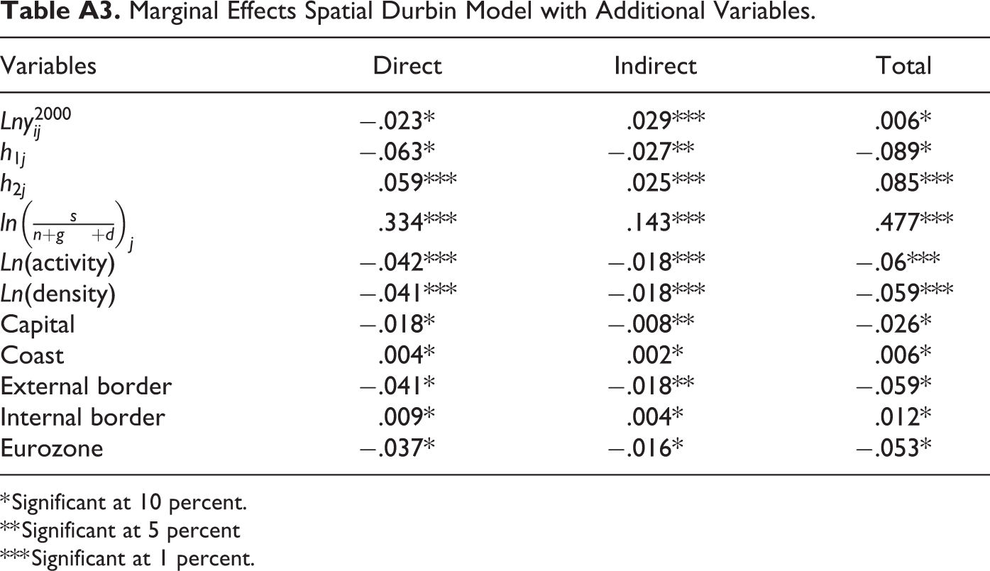
The VPC is 79.8 percent, showing that the hierarchy could be of central importance in the process of convergence in the EU. The robustness of the VPC estimation was verified using a model with additional variables, which are not in the Ertur and Koch (2007) model, like activity rates, densities and dummy regions with a national capital, internal border, external border, coastline, and Eurozone membership. Table A2 of Appendix A indicates that the conclusions from the VPC are the same. The hierarchy is central to the process of convergence, even when including the additional variables.

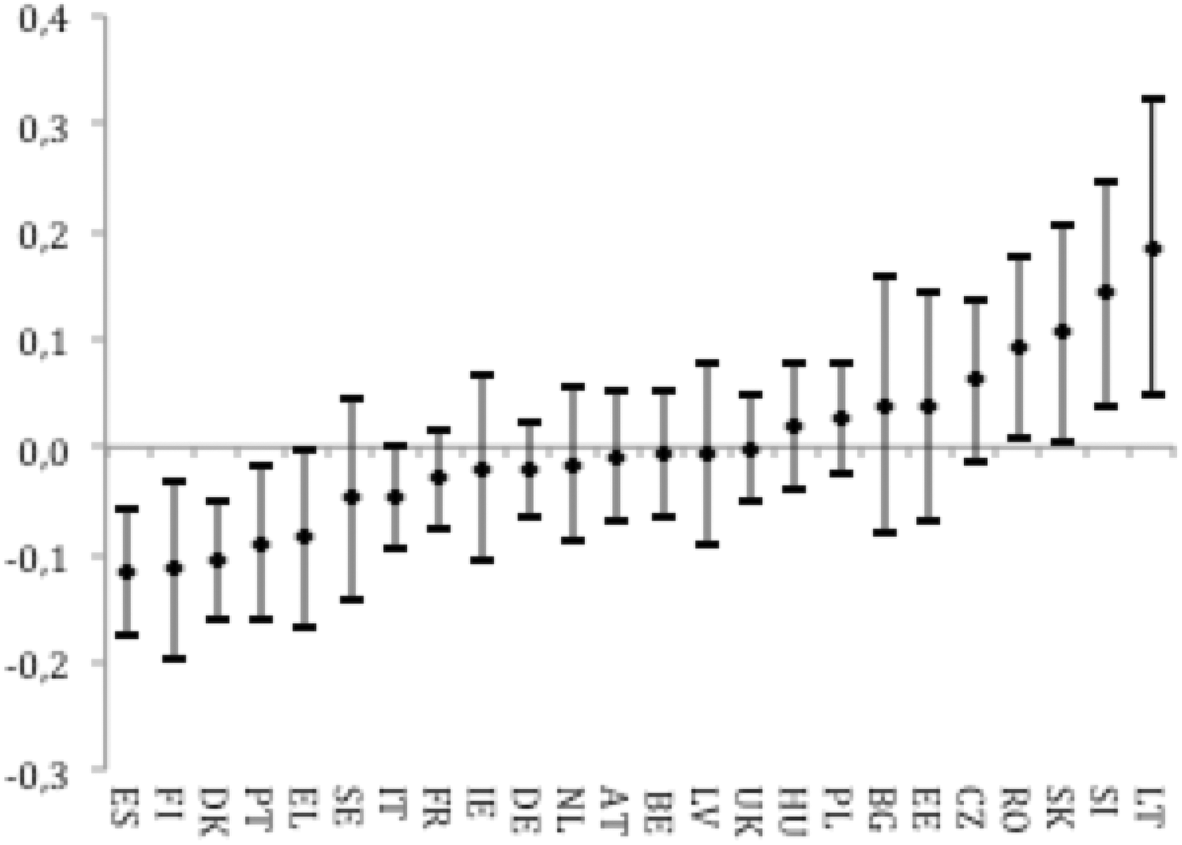
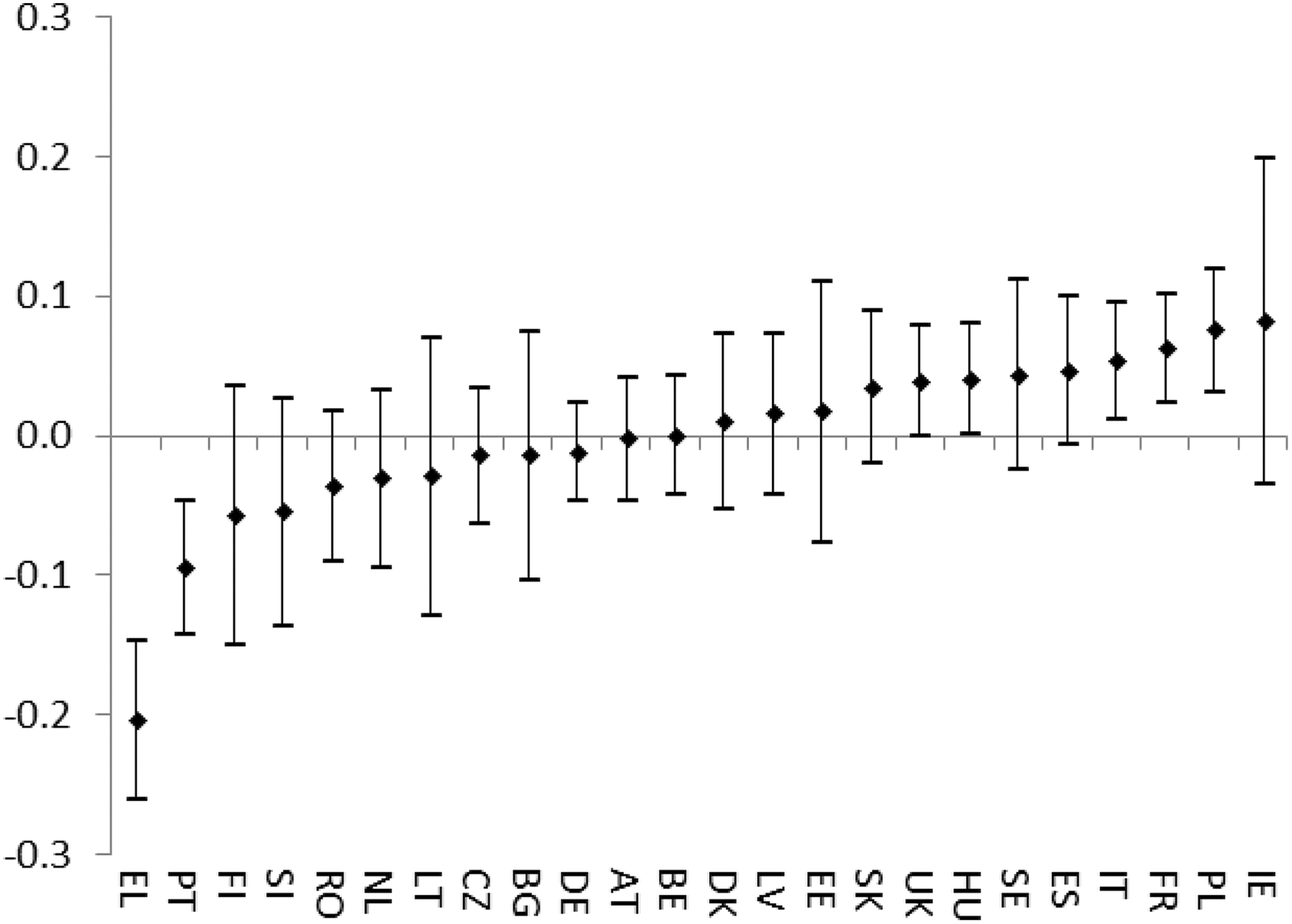
An interesting result using this spatial multilevel model is that we can also find the intercept and slope for each country. These parameters are obtained for the last model in a second estimation following the procedure explained in Goldstein (2011). A brief explanation of this procedure can be found in Appendix B for further details. They indicate whether a country has a significantly different estimate than the common estimate. To explore the variations among countries, the slopes could be considered instances of convergence in one country away from the general process. By contrast, the intercepts represent the steady state of a country when the remaining variables are 0. The slopes and intercepts found using the extended multilevel SDM model are shown in Figures 2 and 3, respectively.

Figure 2.

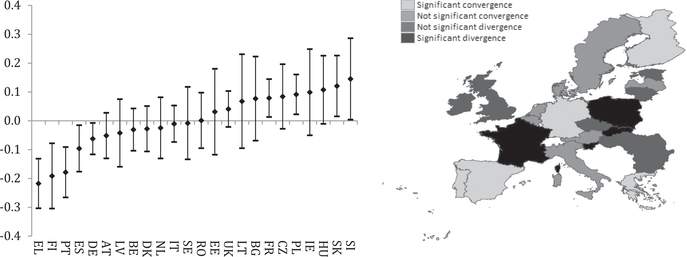
Country specific slopes (v_j ) in the random slope model with spatial effects.

Figure 3.

Intercepts by country in the random slope model with spatial effects.

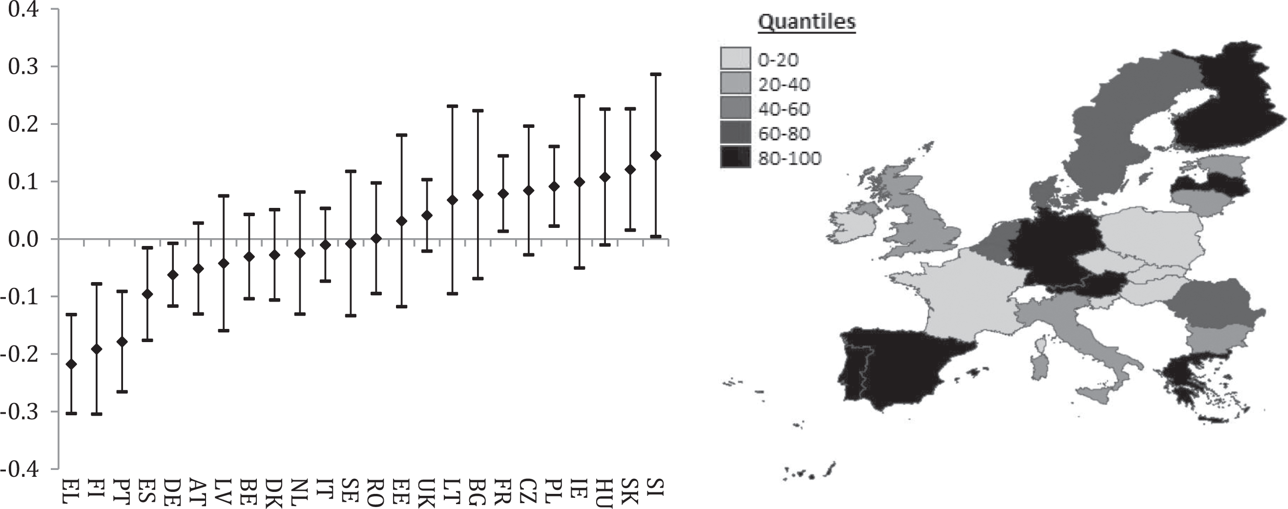
The country-specific estimates show significant differences among the convergence behavior of the countries of the EU. For example, countries such as France, Ireland, and Slovenia have an internal process of significant divergence, whereas others, such as Spain, Greece, and Portugal, have an internal process of significant convergence. By means of this information and the common slope of $L n (y^{2000})$ , the final implied rate of convergence for each country can be obtained. This information can be seen in Appendix A (last column of Table A1).

In addition to the differences in the speed of convergence among countries, there are significant differences in the intercepts among countries. A significant heterogeneity in the intercepts indicates that the process of convergence in the EU could end in a final theoretical equilibrium with significant differences in the GDPpc between countries. This evidence could represent a problem of integration among the countries of the model due to significant differences that the process of convergence cannot correct.

The results show that the new EU members are defined by a higher rate of growth after taking other factors into account. The convergence rates of these countries are lower than those of the other countries in the EU. Artelaris, Kallioras, and Petrakos (2010) show that the communist period of these new member countries created a large homogeneity of wealth. Therefore, they are becoming similar to the other EU countries in terms of both wealth and spatial inequalities.

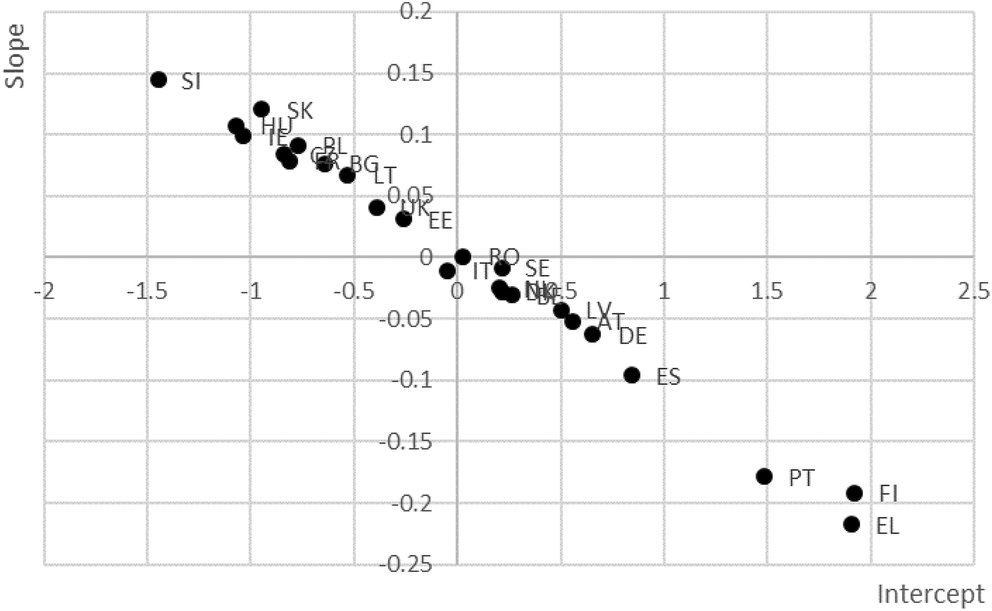
The cases can be visualized using a scatter plot of the intercepts and slopes of the countries. Figure 4 shows the joint distribution of slopes and intercepts in the European scenario. This graph divides the scenarios using a faster or slower process of convergence and the intercept, which is the potential of the economy. This figure highlights a negative relationship between the intercept and the slope. This result indicates that countries that are near to (far from) their steady state could increase (decrease) inequalities within their territory.

Figure 4.

Scatter plot of the intercepts and the slopes.

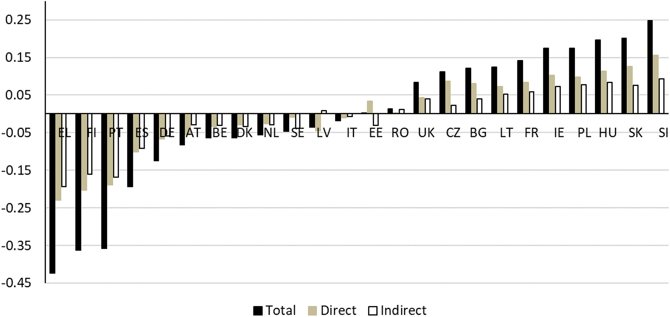
As explained in LeSage and Pace (2009), the effect of the variables in an SDM can be decomposed into direct, indirect, and total effects. The marginal effects for the common coefficients described in Table 2 are summarized in Table 4. These effects indicate the derivate for the variables of interest, including the spatial interactions that may exist through the spatial interactions presented by the spatial weight matrix. As in the Table 2, the decomposition confirms that the common process of convergence is relatively slow and insignificant in a multilevel context.

Table 4.

Marginal Effects Spatial Durbin Model.

Variables	Direct	Indirect	Total
$L n (y^{2000})$	−.027	−.007	−.034
h ₁	−.043	−.059***	−.102**
h ₂	.055*	−.02***	.035*
$L n (\frac{s}{n + g + d})$	.275***	.144	.419*

Note: Inference obtained through simulation with 1,000 trials.

* Significant at 10 percent.

** Significant at 5 percent

*** Significant at 1 percent.

In addition to the decomposition represented in Table 4, the variation in the direct, indirect, and total effects of $L n (y^{2000})$ through the component of country-specific slopes (v_j ) can also be obtained. It is estimated through ${(I - ρ W)}^{- 1} diag (v_{j})$ , where $diag (v_{j})$ is a diagonal matrix of the country-specific slopes applied in each region. Following the decomposition for the common term, the direct effect is the mean of the elements in the diagonal for the regions in country j. The total effect is the mean of the row sums in the different regions in each country j. The indirect effect is obtained as the difference between the total and direct effects.

These effects are summarized in Figure 5 and mapped in Figures 6 –8. The representations of the effects seem to confirm that the marginal effect through the common coefficients is relatively small compared to the wide variability of the marginal effects among the EU countries. This result confirms that the process of convergence is strongly influenced by the country of the region. In fact, this hierarchically organized process of convergence may indicate a lack of integration between the different EU countries toward a unified model of growth and convergence.

Figure 5.

Variation in the marginal effects of $L n (y^{2000})$ by country.

Figure 6.

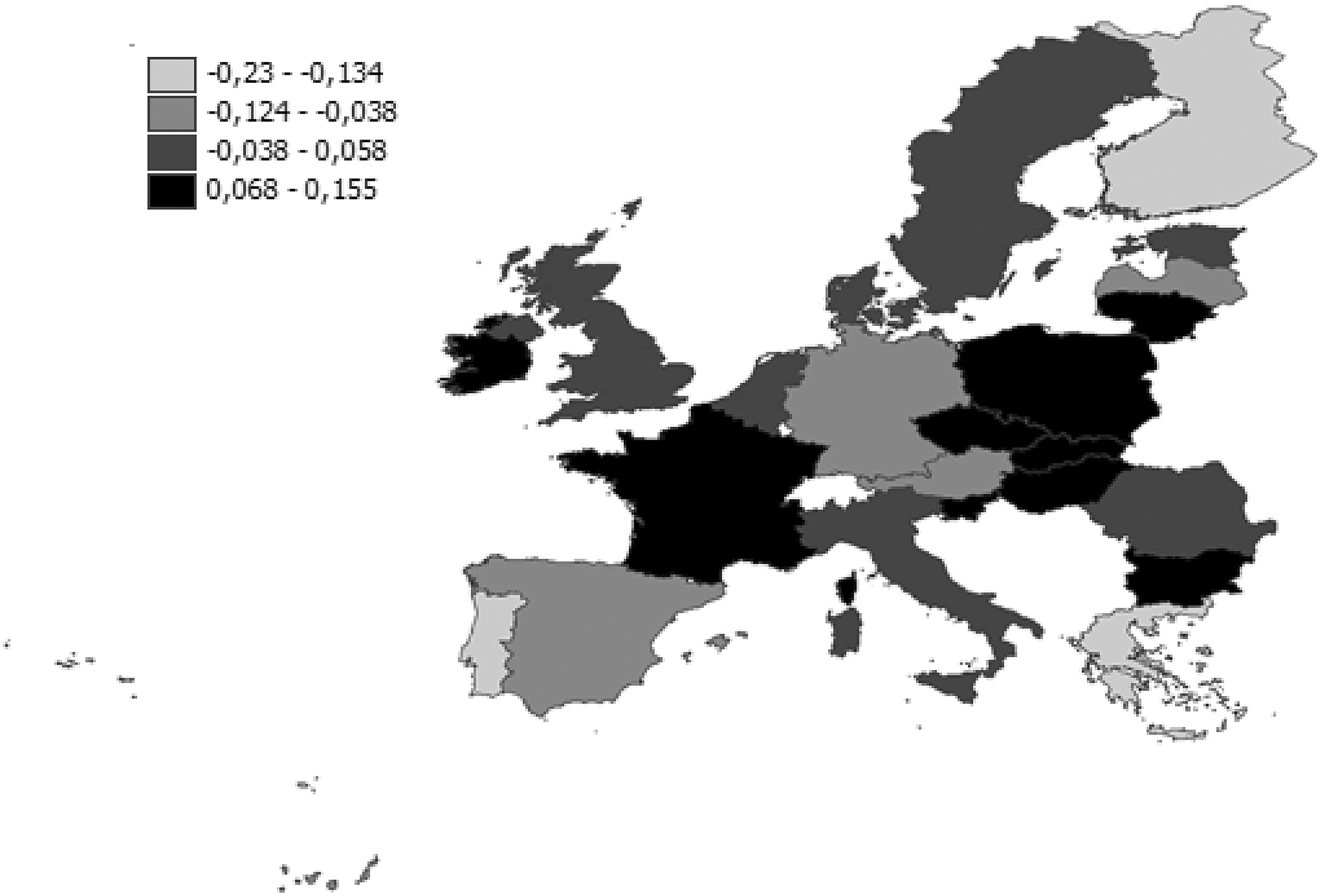
Variation in the direct effects by country.

Figure 7.

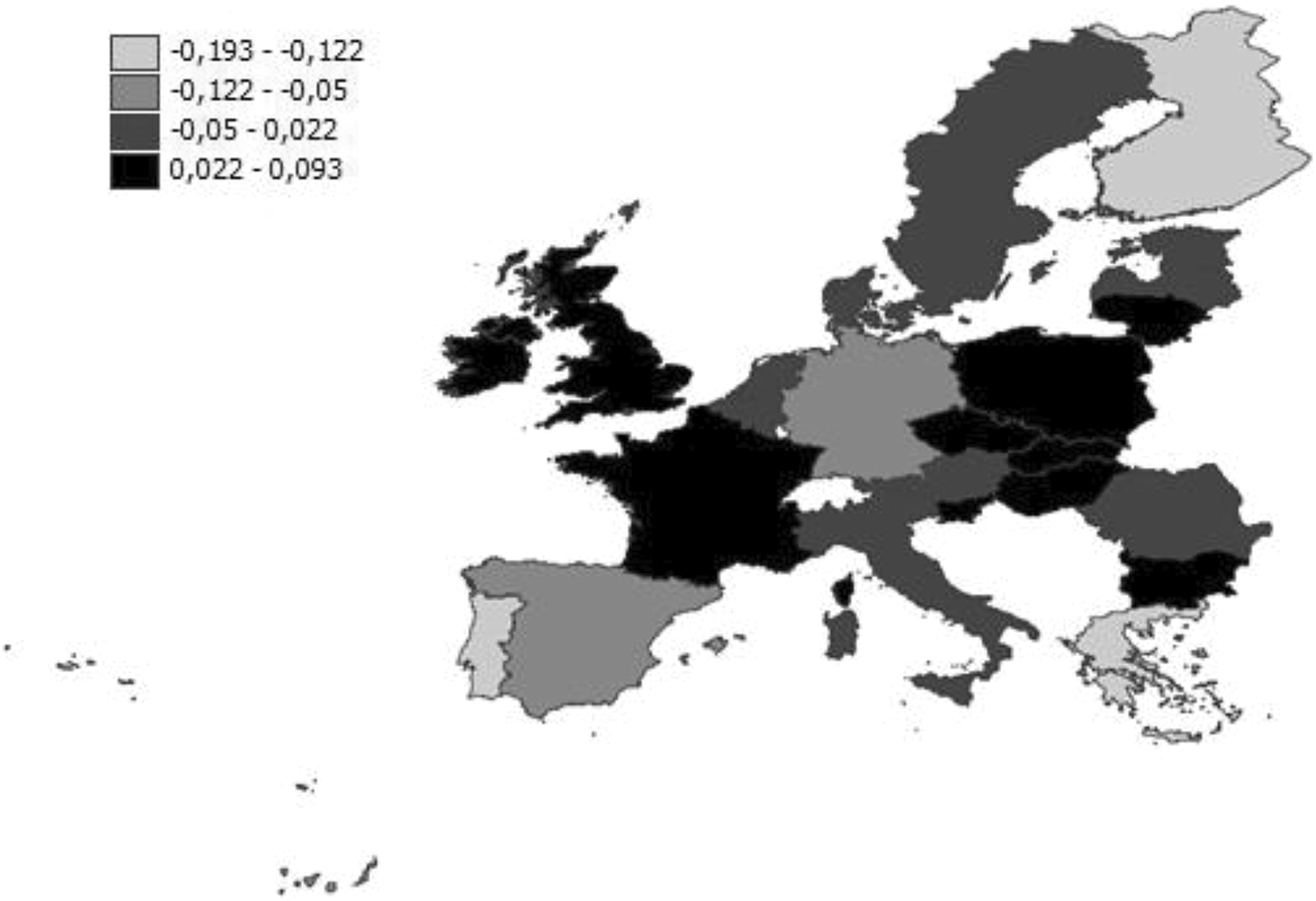
Variation in the indirect effects by country.

Figure 8.

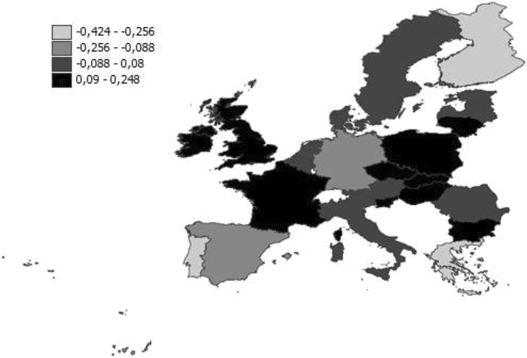
Variation in the total effects by country.

This main result is completely coherent with the ones obtained in previous analysis of convergence clubs for the EU when the authors consider spatially desegregated data and potential heterogeneity in the convergence patterns. For instance, in Postiglione, Andreano, and Benedetti (2013), a procedure for the identification of convergence clubs in EU at NUTS-II level accepting potential spatial heterogeneity is presented, reaching very similar conclusions about the existence of different national convergence behaviors hidden under the aggregated analysis. Postiglione, Benedetti, and Lafratta (2010); Le Gallo and Dall’erba (2006); and Quah (1997), among others, also anticipate similar conclusions.

Results II: Impact of the Great Economic Recession

The great international economic recession that started in 2008 has had a significant impact on the growth of Europe as a whole, as well as on individual countries and regions in the EU. Taking advantage of the fact that the available data cover most of the recession period, we can round out our study by conducting a specific analysis of the crisis’ impact on the convergence dynamics by applying a multilevel approach with spatial effects. To this end, Tables 5 and 6 present the five proposed estimated models, dividing the estimation period into a precrisis phase (2000–2007) and a crisis phase (2008–2014).

Table 5.

Random Slope Model of Unconditional and Conditional $β$ -Convergence of the NUTS-III (2000–2007).

Variables	(1) Unconditional OLS	(2) Conditional OLS	(3) Unconditional Random Slope	(4) Conditional Random Slope	(5) Random Slope SDM
Constant	0.64***	−0.465***	0.29	−0.248	−0.17
$L n (y^{2000})$	−0.05***	−0.021***	−0.002	−0.012	−0.007
$L n h_{1}$		0.016**		−0.004	−0.01
$L n h_{2}$		0.12***		0.052***	0.042***
$L n (\frac{s}{n + g + d})$		0.279***		0.309***	0.23**
W $L n (y^{2000})$					0.009
W $L n h_{1}$					−0.01
W $L n h_{2}$					−0.02
W $L n (\frac{s}{n + g + d})$					−0.053
Rho					0.605***
$S D (v_{0 j})$			1.116	1.11	1.162
$S D (v_{1 j})$			0.132	0.13	0.133
$cov (v_{0 j}, v_{1 j})$			−0.144	−0.142	−0.153
Mean VPC (percent)			93.58	93	91.02
N	1,276	1,276	1,276	1,276	1,276
M			24	24	24
Speed of general convergence (percent)	0.73	0.27	0.01	0.17	0.09
Adjusted R ² (percent)	22.91	46.52

Note: SD = standard deviation; OLS = ordinary least squares; VPC = variance partition coefficient; SDM = spatial Durbin model.

* Significant at 10 percent.

** Significant at 5 percent

*** Significant at 1 percent.

Table 6.

Random Slope Model of Unconditional and Conditional $β$ -Convergence of the NUTS-III (2008–2014).

Variables	(1) Unconditional OLS	(2) Conditional OLS	(3) Unconditional Random Slope	(4) Conditional Random Slope	(5) Random Slope SDM
Constant	0.119***	−0.326***	0.23	0.344	0.417
$L n (y^{2008})$	−0.013***	−0.014***	−0.025	−0.023	−0.025
$L n h_{1}$		0.107***		−0.017	−0.022
$L n h_{2}$		0.031***		−0.011	−0.001
$L n (\frac{s}{n + g + d})$		−0.034***		−0.022	−0.017
W $L n (y^{2008})$					−0.001
W $L n h_{1}$					0.004
W $L n h_{2}$					−0.022*
W $L n (\frac{s}{n + g + d})$					−0.006
Rho					0
$S D (v_{0 j})$			1.039	1.042	1.03
$S D (v_{1 j})$			0.107	0.107	0.105
$cov (v_{0 j}, v_{1 j})$			−0.11	−0.111	−0.108
Mean VPC (percent)			86.09	86.94	85.2
N	1,276	1,276	1,276	1,276	1,276
M			24	24	24
Speed of general convergence (percent)	0.19	0.20	0.36	0.33	0.36
Adjusted R ² (percent)	2	22.07

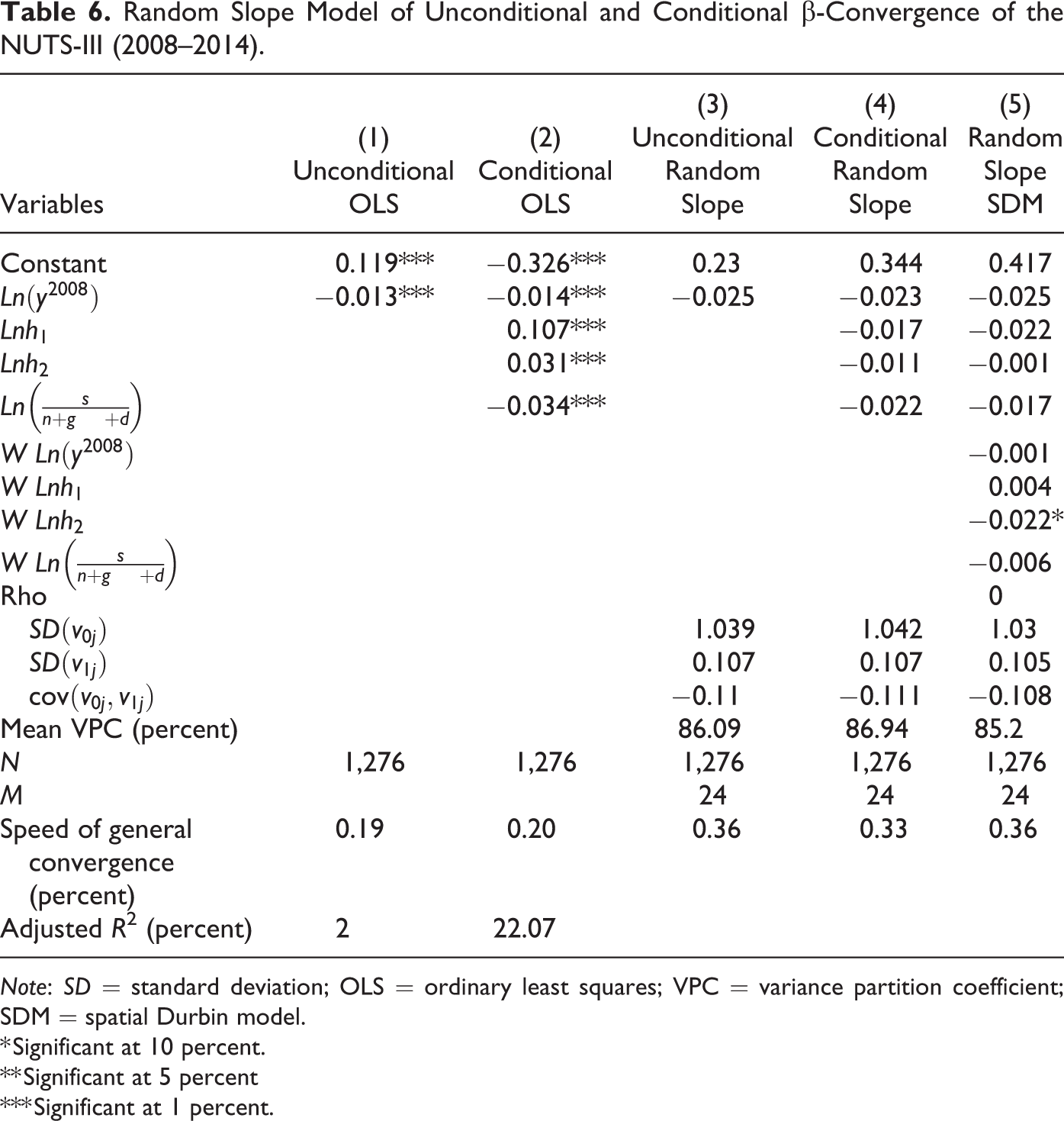
Note: SD = standard deviation; OLS = ordinary least squares; VPC = variance partition coefficient; SDM = spatial Durbin model.

* Significant at 10 percent.

** Significant at 5 percent

*** Significant at 1 percent.

In Table 5, one can see that the general dynamics found in the precrisis phase (2000–2007) are very similar to the dynamics of the entire period. We observed a moderate but significant convergence in the simple OLS models. However, this aggregate convergence disappears when we consider multilevel effects with unconditional random slope (model 3), multilevel effects with conditional random slope (model 4), and multilevel effects with conditional random slope and spatial effects using an SDM specification (model 5). Figure 9 shows the country-specific slopes from model 5, which confirms that the behavior of individual countries is essentially the same as in the general model. The rho parameter is significant, indicating that there are spatial effects. Table 3 presents the marginal effects from the SDM specification, which, as shown, are very similar to those identified for the entire period.

Figure 9.

Country specific slopes (v_j ) in the random slope model with spatial effects (2000–2007).

However, these conclusions change during the economic crisis period (2008–2014), as seen in Table 6. Although convergence remains significant in the OLS specification, it is clearly reduced and has a very low convergence speed (0.17 percent in the unconditional model and 0.21 percent in the conditional model). This aggregate convergence disappears again under all of the multilevel specifications. Focusing on the most complete model (model 5), we can see that there is no aggregate convergence nor are most of the control variables significant. Likewise, the special effect of the rho parameter is no longer significant (which is why we do not present the table of marginal effects). Figure 10 shows the country-specific slopes from the results of model 5. As the figure shows, there are several cases in which internal convergence ceases to be significant, and some countries that are heavily affected by the crisis, such as Spain, go from having significant internal convergence to equally significant internal divergence. Although it is too early to know how the international economic crisis affected the dynamics of convergence in Europe, everything seems to indicate that the already weak convergence before the crisis became even weaker after the impact of the Great Recession.

Figure 10.

Country specific slopes (v_j ) in the random slope model with spatial effects (2008–2014).

Conclusion

Economic convergence studies, especially those that use the β-convergence approach, are important not only because they offer a precise image of the evolution of the economic disparities among territories but also because they are a method of testing neoclassical economic growth models. However, in the case of the EU, these types of convergence studies have a special relevance for several reasons. First, the persistence of large income and economic development disparities (e.g., Magrini 1999; Giannetti 2002) among EU countries and regions are challenging the stability of the monetary union and even the entire EU integration project. Second, given that EU institutions are conscious of the importance of reducing the disparities among territories, they have implemented the European Cohesion Policy, which is one of the most important EU policies. In budgetary terms, it represented one-third of all expenditures in 2016. Third, the European case is especially interesting due to the complexity from the spatial perspective. Different behaviors exist at the national and regional levels. Countries can quickly converge with the rest of the Union and with areas that have a lower capacity for growth and vice versa, in addition to different political decision levels.

In this article, a usual β-convergence equation has been estimated using a multilevel method combined with spatial models, allowing us to further explore the complexity of the processes of convergence among countries and large regions. Using this type of estimation, several processes of convergence of each country have been calculated that take into account the general process for the entire sample. As a result, the importance of the variance between and within countries, as shown by the β-convergence, can be estimated. For empirical application, we have data for the period 2000–2014. This enables us to offer new, updated evidence for the dynamics of convergence in Europe. By covering the period affected by the great international economic recession, we have also been able to take a first look at the impact of this crisis on the growth and convergence of Europe’s countries and regions.

This methodology has been applied in a framework of cross-sectional analysis. In future analysis, different panel structures—regional as well as country effects, dynamic effects, dynamic spatial effects, or temporal hierarchy—can be used to extend and improve this first approach. In addition, future analysis could explore the effect of the international economic recession using a longer period of analysis.

With our multilevel spatial effect cross-sectional approach, we can reach very interesting conclusions that highlight the importance of the spatial levels in the process of convergence in the EU. There is a general behavior of convergence, but many countries show no evidence of significant internal convergence. This outcome directly contradicts the primary goal of the regional policy of the EU to be a relevant source of asymmetric shocks. To observe whether the differences in the models of convergence are caused by the fundamental factors explained in the neoclassical literature, the estimation was expanded to include new information. However, even with the inclusion of this information, there are still important differences among the countries and the main conclusion of the coexistence of a global moderate convergence with intranational processes of divergence. The crisis has heavily affected the dynamics of convergence. Generally, there is a loss of convergence, and in specific cases, countries go from having internal convergence behaviors to insignificant convergence or even divergence.

In this analysis, we find that the existence of different convergence trends that depend on the spatial level of observation is a relevant phenomenon that must be considered. We also observe how the economic cycle affects dynamics both at an aggregate level and for individual countries. Regional policy should implement both policies to extend the convergence through the entire EU and policies to reduce the intranational divergence processes that could coexist with a general trend of convergence. This is especially relevant due to the existence of discrepancies among national and local behaviors that could be the result of several recent controversial political decisions, as is noted by McCann (2016) in the case of the United Kingdom. In addition, it is especially relevant after the negative impact of the great economic recession over the growth and convergence in Europe.

Footnotes

Appendix A

Table A3.

Marginal Effects Spatial Durbin Model with Additional Variables.

Variables	Direct	Indirect	Total
$L n y_{i j}^{2000}$	−.023*	.029***	.006*
$h_{1 j}$	−.063*	−.027**	−.089*
$h_{2 j}$	.059***	.025***	.085***
$l n {(\frac{s}{n + g + d})}_{j}$	.334***	.143***	.477***
Ln(activity)	−.042***	−.018***	−.06***
Ln(density)	−.041***	−.018***	−.059***
Capital	−.018*	−.008**	−.026*
Coast	.004*	.002*	.006*
External border	−.041*	−.018**	−.059*
Internal border	.009*	.004*	.012*
Eurozone	−.037*	−.016*	−.053*

* Significant at 10 percent.

** Significant at 5 percent

*** Significant at 1 percent.

Appendix B

Declaration of Conflicting Interests

The author(s) declared no potential conflicts of interest with respect to the research, authorship, and/or publication of this article.

Funding

The author(s) disclosed receipt of the following financial support for the research, authorship, and/or publication of this article: This article was funded by IMAJINE—EU Project of the Horizon 2020.

ORCID iD

Fernando Rubiera-Morollon

Notes

References

Abramovitz

1986. “Catching Up, Forging Ahead, and Falling Behind.” The Journal of Economic History 46:385–406.

Abreu

De Groot

Florax

R. J. G. M.

. 2005. “A Meta-analysis of β-convergence: The Legendary 2%.” Journal of Economic Surveys, 19(3): 389–420.

Alexiadis

. 2013. Convergence Clubs and Spatial Externalities: Models and applications of Regional Convergence in Europe. Berlin, Germany: Springer.

Amemiya

(1985). Advanced Econometrics. Cambridge, MA: Harvard University Press.

Andersson

Hammarstedt

Hussain

. 2013. “Ethnic Origin, Local Labour Markets and Self-employment in Sweden: A Multilevel Approach.” The Annals of Regional 50:885–910.

Anselin

. 1988. Spatial Econometrics: Methods and Models. Berlin, Germany: Springer.

Anselin

Florax

R. J. G. M.

. 1995. New Directions in Spatial Econometrics. Berlin, Germany: Springer.

Anselin

Rey

S. J.

. 1997. “Introduction to the Special Issue on Spatial Econometrics.” International Regional Science Review 20:1–7.

Arbia

Petrarca

. 2011. “Effects of MAUP on Spatial Econometric Models.” Letters in Spatial and Resource Sciences 4:173–85.

10.

Artelaris

Kallioras

Petrakos

. 2010. “Regional Inequalities and Convergence Clubs in the European Union New Member-states.” Eastern Journal of European 1(1): 113–33.

11.

Ballas

Tranmer

. 2012. “Happy People or Happy Places? A Multilevel Modeling Approach to the Analysis of Happiness and Well-being.” International Regional Science Review 35:70–102.

12.

Bartkowska

Riedl

. 2012. “Regional Convergence Clubs in Europe: Identification and Conditioning Factors.” Economic Modelling 29:22–31.

13.

Battisti

De Vaio

. 2008. “A Spatially Filtered Mixture of β-convergence Regressions for EU Regions, 1980–2002.” Empirical Economics 34:105–21.

14.

Baumol

W. J.

1986. “Productivity Growth, Convergence, and Welfare: What the Long-run Data Show.” The American Economic Review 76:1072–85.

15.

Canova

Marcet

. 1995. “The Poor Stay Poor: Non-convergence across Countries and Regions.” London CEPR Discussion Papers, 1265, 1–37.

16.

Castellacci

Los

de Vries

G. J.

. 2014. “Sectoral Productivity Trends: Convergence Islands in Oceans of Non-convergence.” Journal of Evolutionary Economics 24:983–1007.

17.

Chasco

López

A. M.

. 2009. “Multilevel Models: An Application to The Beta-convergence Model.” Region et Developpement 30:35–58.

18.

Cheshire

Carbonaro

. 1996. “Urban Economic Growth in Europe: Testing Theory and Policy Prescriptions.” Urban Studies 33:1111–28.

19.

Cohen

P. N.

1998. “Black Concentration Effects on Black-white and Gender Inequality: Multilevel Analysis for US Metropolitan Areas.” Social Forces 77:207–29.

20.

Corrado

Fingleton

. 2012. “Where is the Economics in Spatial Econometrics?” Journal of Regional Science 52:210–39.

21.

Coulombe

Lee

. 1993. Regional Economic Disparities in Canada. Ottawa, Canada: University of Ottawa.

22.

Cuadrado-Roura

J. R.

García-Greciano

Raymond

J. L.

. 1999. “Regional Convergence in Productivity and Productive Structure: The Spanish Case.” International Regional Science Review 22:35–53.

23.

De la Fuente

2002. “On the Sources of Convergence: A Close Look at the Spanish Regions.” European Economic Review 46:569–99.

24.

Díaz-Dapena

Fernández-Vázquez

Rubiera-Morollón

. 2016. “The Role of Spatial Scale in Regional Convergence: The Effect of MAUP in the Estimation of Beta-convergence Equations.” The Annals of Regional Science 56:473–89.

25.

Díaz-Dapena

Rubiera-Morollón

Paredes-Araya

. 2017. “Are There Different Local Patterns of Convergence Concealed beneath the Regional Level? An Analysis for US States and Counties Using a Multilevel Approach.” The Annals of Regional Science 58:623–40.

26.

Díaz-Dapena

Rubiera-Morollón

Pires

Gomes

. 2017. “Convergence in Brazil: New Evidence Using a Multilevel Approach.” Applied Economics 49:5050–62.

27.

Duncan

Jones

Moon

. 1998. “Context, Composition and Heterogeneity: Using Multilevel Models in Health Research.” Social Science & Medicine 46:97–117.

28.

Durlauf

S. N.

2000. Econometric Analysis and the Study of Economic Growth: A Skeptical Perspective. Madison: Social Systems Research Institute, University of Wisconsin.

29.

Durlauf

S. N.

Johnson

P. A.

. 1995. “Multiple Regimes and Cross-country Growth Behaviour.” Journal of Applied Econometrics 10:365–84.

30.

Elhorst

J. P.

2010. “Applied Spatial Econometrics: Raising the Bar.” Spatial Economic Analysis 5:9–28.

31.

Elhorst

J. P

. 2014. Spatial Econometrics: From Cross-sectional Data to Spatial Panels. Berlin, Germany: Springer.

32.

Elhorst

J. P.

Piras

Arbia

. 2010. “Growth and Convergence in a Multiregional Model with Space–Time Dynamics.” Geographical Analysis 42:338–55.

33.

Elhorst

J. P.

Zeilstra

A. S.

. 2007. “Labour Force Participation Rates at the Regional and National Levels of the European Union: An Integrated Analysis.” Papers in Regional Science 86:525–49.

34.

Ertur

Le Gallo

. 2009. “Regional Growth and Convergence: Heterogeneous Reaction versus Interaction in Spatial Econometric Approaches.” In Handbook of Regional Growth and Development Theories, edited by Capello

Nijkamp

, 374–88. Northampton, UK: Edward Elgar.

35.

Ertur

Koch

. 2007. “Growth, Technological Interdependence and Spatial Externalities: Theory and Evidence.” Journal of Applied Econometrics 22:1033–62.

36.

Escriba

Murgui

M. J.

. 2014. “La base de datos BD.EURS (NACE Rev.1).” Investigaciones Regionales 28:173–94.

37.

Frees

E. W

. 2004. Longitudinal and Panel Data: Analysis and Applications in the Social Sciences. Cambridge, MA: Cambridge University Press.

38.

Fujita

Krugman

. 1995. “When is the Economy Monocentric? von Thünen and Chamberlin Unified.” Regional Science and Urban Economics 25:505–28.

39.

Fujita

Krugman

Venables

. 2001. The Spatial Economy: Cities, Regions, and International Trade. Cambridge, MA: MIT Press.

40.

Gehlke

C. E.

Biehl

. 1934. “Certain Effects of Grouping upon the Size of the Correlation Coefficient in Census Tract Material.” Journal of the American Statistical Association 29:169–70.

41.

Giannetti

2002. “The Effects of Integration on Regional Disparities: Convergence, Divergence or Both?” European Economic Review 46:539–67.

42.

Goldstein

1986. “Multilevel Mixed Linear Model Analysis Using Iterative Generalized Least Squares.” Biometrika 73:43–56.

43.

Goldstein

2011. Multilevel Statistical Models. Chichester, UK: John Wiley.

44.

Hox

2010. Multilevel Analysis: Techniques and Applications. New York: Routledge.

45.

Islam

1995. “Growth Empirics: A Panel Data Approach.” The Quarterly Journal of Economics 110:1127–70.

46.

Islam

2003. “What Have We Learnt from the Convergence Debate?” Journal of Economic Surveys 17:309–62.

47.

Kelejian

H. H.

1974. “Random Parameters in a Simultaneous Equation Framework: Identification and Estimation.” Econometrica: Journal of the Econometric Society 42(3):517–27.

48.

Kelejian

H. H.

Prucha

I. R.

Yuzefovich

. 2004. “Instrumental Variable Estimation of a Spatial Autoregressive Model with Autoregressive Disturbances: Large and Small Sample Results.” Advances in Econometrics 18:163–98.

49.

Krugman

1991. “Increasing Returns and Economic Geography.” The Journal of Political Economy 99:483–99.

50.

Krugman

Venables

A. J.

. 1995. “Globalization and the Inequality of Nations.” The Quarterly Journal of Economics 110:857–80.

51.

Lacombe

D. J.

McIntyre

S. G.

. 2017. “Hierarchical Spatial Econometric Models in Regional Science.” In Regional Research Frontiers, Vol. 2, edited by Randall

Peter

, 151–67. Berlin, Germany: Springer.

52.

Le Gallo

Dall’erba

. 2006. “Evaluating the Temporal and Spatial Heterogeneity of the European Convergence Process, 1980-1999.” Journal of Regional Science 46:269–88.

53.

LeSage

Pace

R. K.

. 2009. Introduction to Spatial Econometrics Statistics: A Series of Textbooks and Monographs. New York: Taylor & Francis Group.

54.

Wei

Y. H. D.

. 2010. “The Spatial-temporal Hierarchy of Regional Inequality of China.” Applied Geography 30:303–16.

55.

López-Bazo

Vayá

Artís

. 2004. “Regional Externalities and Growth: Evidence from European Regions.” Journal of Regional Science 44:43–73.

56.

Magrini

1999. “The Evolution of Income Disparities among the Regions of the European Union.” Regional Science and Urban Economics 29:257–81.

57.

Magrini

. 2004. “Regional (di) Convergence.” In Handbook of Regional and Urban Economics, edited by Henderson

J. V.

Nijkamp

Mills

E. S.

Cheshire

P. C.

Thisse

J. F.

Vol. 4, 2741–96. North Holland, the Netherlands: Elsevier.

58.

Mankiw

N. G.

Romer

Weil

D. N.

. 1992. “A Contribution to the Empirics of Economic Growth.” The Quarterly Journal of Economics 107:407–37.

59.

McCann

2016. The UK Regional–National Economic Problem: Geography, Globalisation and Governance. New York: Taylor & Francis Group.

60.

Mella-Marquez

J. M.

Chasco-Yrigoyen

. 2006. “A Spatial Econometric Analysis of Urban Growth and Territorial Dynamics: A Case Study on Spain.” In Spatial Dynamics, Networks and Modelling, edited by Reggiani

P. N. A.

, 325–66. Northampton, UK: Edward Elgar.

61.

Monfort

Cuestas

Ordonez

. 2013. “Real Convergence in Europe: A Cluster Analysis.” Economic Modelling 33:689–94.

62.

Openshaw

1984. The Modifiable Areal Unit Problem, Concepts and Techniques in Modern Geography. Norwich, UK: Geo Books.

63.

Openshaw

Taylor

. 1979. “A Million or So Correlation Coefficients.” In Statistical Methods in the Spatial Sciences, edited by Wrigley

, 127–44. London, UK: Pion.

64.

Postiglione

Andreano

Benedetti

. 2013. “Using Constrained Optimization for the Identification of Convergence Clubs.” Computational Economics 42:151–74.

65.

Postiglione

Benedetti

Lafratta

. 2010. “A Regression Tree Algorithm for the Identification of Convergence Clubs.” Computational Statistics & Data Analysis 54:2776–85.

66.

Quah

D. T.

1997. “Empirics for Growth and Distribution: Stratification, Polarization, and Convergence Clubs.” Journal of Economic Growth 2:27–59.

67.

Ramajo

Márquez

M. A.

Hewings

G. J. D.

Salinas

M. M.

. 2008. “Spatial Heterogeneity and Interregional Spillovers in the European Union: Do Cohesion Policies Encourage Convergence across Regions?” European Economic Review 52:551–67.

68.

Rey

S. J.

Le Gallo

. (2009). “Spatial Analysis of Economic Convergence.” In Palgrave Handbook of Econometrics, edited by Mills

T. C.

Patterson

. London, UK: Palgrave Macmillan.

69.

Rey

S. J.

Montouri

B. D.

. 1999. “US Regional Income Convergence: A Spatial Econometric Perspective.” Regional Studies 33:143–56.

70.

Sala-I-Martin

1994. “Cross-sectional Regressions and the Empirics of Economic Growth.” European Economic Review 38:739–47.

71.

Shioji

. 1992. Regional Growth in Japan. New Haven, CT: Yale University.

72.

Srholec

2010. “A Multilevel Approach to Geography of Innovation.” Regional Studies 44:1207–20.

73.

Stakhovych

Bijmolt

T. H. A.

. 2009. “Specification of Spatial Models: A Simulation Study on Weights Matrices.” Papers in Regional Science 8(2): 389–408.

74.

Swamy

. 1970. “Efficient Inference in a Random Coefficient Regression Model.” Econometrica: Journal of the Econometric Society 38(2): 311–23.

75.

Zeilstra

A. S.

Elhorst

J. P.

. 2014. “Integrated Analysis of Regional and National Unemployment Differentials in the European Union.” Regional Studies 48:1739–55.