The Vertical and Horizontal Equity of Property Assessment Caps

Abstract

Do assessment caps make the property tax more regressive? Are they fair to all taxpayers, or do some groups get more benefit than others. This paper examines these issues using a sample from the Jacksonville, FL Metropolitan Statistical Area. Regression models are run using housing values averaged at the census block level and matched to census block socioeconomic and demographic data obtained from the US Census. Results show that when permanent income is used as the measure of ability to pay, the SOH benefit makes the property tax fairer, but when current income is used as the income measure, it makes the tax less fair. In addition, the assessment caps cause some serious horizontal inequities. For, example, homes in 100% Black census blocks receive, on average, 6.6 percentage points less value from the SOH benefit relative to their home’s value than the homes in 100% White census blocks.

Keywords

property tax horizontal equity vertical equity assessment caps racial differences

Introduction

The property tax is the primary revenue source for most local governments. In fiscal year 2019, property taxes made up 31% of total U.S., state, and local tax collections, and 72% of local tax collections nationwide (Cammenga 2021). When a revenue source is this ubiquitous, it’s important to understand who’s paying the tax, and if the burden of the tax is distributed fairly.

Assessment caps can significantly affect homeowners’ tax burdens. California took the lead in placing caps on property tax assessments in 1978 with the institution of Proposition 13. Since that time many states have followed suit. In 2020, 18 states plus the District of Columbia had caps on the amount that assessment values can increase in a year (Walczak 2020). In 1992, voters in Florida passed the Save Our Homes (SOH) Amendment that limits property assessment increases to 3% per year or the annual inflation rate, whichever is lower. In 2007, Florida voters passed another amendment that made the amount of SOH savings portable. Property owners can now transfer the difference between the market value and the assessed value of their properties (up to a maximum of $500,000 in 2021) to another property that they buy.

This has a huge effect on property taxes in Florida. In 2020, the difference between market (just) values and assessed values for real property in Florida’s 67 counties was over $313.27 billion (Florida Department of Revenue 2020). Based on the average effective property tax rate for Florida counties in 2020, this amounted to approximately $3.95 billion in lost tax revenue (smartasset.com 2021). Although policymakers recognize the size and growing importance of assessment cap initiatives, very little is known about who is receiving these tax breaks and whether they are equitably distributed across different demographic and socioeconomic groups.

This paper hopes to shed light on this issue by examining both the vertical and horizontal equity of the SOH tax preference. There should be no distinction between a tax or a tax savings in terms of equity: both should face the same equity principles. Stiglitz and Rosengard (2015) analyze tax breaks by calling them tax expenditures. They emphasize that anytime Congress or voters pass a tax preference, it is equivalent to spending tax dollars (it has the same effect on the government’s budget as an equal amount of new spending). Vertical equity measures how tax rates differ across income groups, and whether the taxes are progressive, regressive, or proportional. Our paper examines vertical equity relative to taxpayers’ permanent as well as current income. There is still some disagreement among economists over which income measure (current vs. permanent) should be used to determine the incidence of the property tax. Thus, we believe our research contributes to the literature by using both income measures so that comparisons can be made regarding the equity of the property tax relative to both income measures.

The paper also examines the horizontal equity of the SOH benefit. Musgrave’s (1961) definition of horizontal equity states that “people in equal positions should be treated equally” (p.1 60). This is interpreted to mean that households with similar characteristics should bear similar tax burdens. All else equal, when households that differ in age, race, ethnicity, or educational attainment pay significantly different tax amounts, this violates the principle of horizontal equity. We believe the emphasis our study places on horizontal equity, especially regarding race, is an important contribution to the property tax literature. It is especially relevant given the recent national attention to the problem of racial differences in property appraisals (Narragon et al. 2021; Kamin 2020; Mock 2020, 2021; Perry, Rothwell, and Harshbarger 2018).

Literature on Property Tax Vertical and Horizontal Equity

The property tax remains one of the least understood taxes when it comes to judging its vertical and horizontal equity. Although the fairness of the tax can be assessed relative to the value of the property itself, the fairness of the tax cannot be assessed relative to the characteristics of the people who pay it. One of the first things a budding tax analyst learns is that people, not sales, gasoline, or in this case, properties, pay taxes, so the true incidence of the tax, rather than the statutory incidence of the tax, must be ascertained. The property tax’s statutory incidence is quite straightforward; the property owner pays the tax. However, property tax records do not include information about the property owner’s income or socioeconomic characteristics, which are the factors used to assess the equity implications of a tax. Characteristics such as the homeowner’s current income, education level, age, race, and ethnicity are missing from the property appraiser’s website.

Another reason that the incidence of the property tax is hard to pin down is that in some cases the property tax may not be viewed as a tax at all, but rather as a user fee that homeowners are willing to pay to receive a bundle of public services that they desire from local government. Tiebout (1956) was the first to propose that citizens vote with their feet by choosing to locate in a community that provides public goods and services, like public schools, police protection, parks, and other amenities, that suit their preferences. In this case, economists don’t need to study the incidence of the property tax because homeowners are getting what they paid for, just like they do for private sector goods. Thus, the property tax is a benefits tax.

However, the Tiebout Hypothesis is a limited case that is only available to people who live in a large metropolitan area with numerous suburbs from which to choose and the necessary income to buy a home in that suburb. Most homeowners view the property tax as a tax, not a user fee, so it’s important to determine its incidence. Economists have determined that the incidence of the tax depends on the use of the property (Aaron 1974; Mieszkowski 1967; Zodrow 2001). For example, if the property is used to generate rental income, then some of the tax will be passed on to renters. In this case, part of the tax will be paid by the renters, making the property tax regressive since housing consumption as a proportion of a household’s income declines with increases in income. This is the so-called traditional view of the incidence of the property tax that held sway over the economics profession in the first half of the 20th century.

It was a reasonable view of property tax incidence when most people did not own their homes, but after World War II, government programs like the FHA and the GI Bill made it much more affordable to buy a home. If the homeowners are occupying the house themselves, then the tax can be viewed as a tax on the capital that the homeowners are accumulating in their homes. In this case, the tax is progressive since capital accumulation increases as income increases. In the general equilibrium view, the property tax is a tax on all capital since the rates of return on all forms of capital will equalize over time. In this case, again, the tax would be progressive since capital accumulation increases with income. Our data include only houses that have been granted the homestead exemption; thus, they are all owner-occupied. This means that the tax should be viewed as a tax on capital. Therefore, we are trying to determine how the SOH assessment cap affects the distribution of the tax on capital accumulated in owner-occupied homes.

In spite of the dearth of information on individual homeowners’ incomes, economists have been able to estimate the vertical equity of the property tax using a Suits Index (Beal, Borg, and Stranahan 2017; Metcalf 1993; Phares 1980; Plummer 2003; Suits 1977). A Suits Index uses a Lorenz curve to compare the cumulative distribution of the tax burden to the cumulative distribution of income. The index takes on values from −1 (perfectly regressive) to +1 (perfectly progressive) with a value of zero indicating a perfectly proportional tax. The index is a broad, aggregate measure that compares the proportion of property tax paid by each decile (10%) of households to the proportion of income earned by each decile of households. As mentioned previously, there is disagreement among researchers about whether to use measures of current income or permanent income in the calculation of the cumulative income distribution used to estimate the Suits Index (Metcalf 1993). Current income is estimated from census data and permanent income is proxied by the market values of the taxed properties. However, from a practical standpoint, empirical results suggest that the use of permanent versus current income made little difference in the size of the estimated Suits indexes. Three studies that used current income (Metcalf 1993; Phares 1980; Suits 1977) found that property taxes had no clear pattern of progressivity or regressivity, with the Suits index ranging from +0.23 (slightly progressive) to −0.23 (slightly regressive) in these studies. Similarly, two studies (Metcalf 1993; Plummer 2003) that used permanent income (proxied by market value of the homes), also showed wide variation, with Suits indexes that ranged from −0.11 to +0.26. Overall, these studies provide no clear consensus about whether property taxes are progressive, proportional, or regressive.

In the real estate literature, studies on vertical equity focus on whether average tax rates vary across the tax base (property values) due to under- or over-valuation during assessment. These studies measure differences in the assessment to sales price ratio (Assessed Value/Sales Value) across neighborhoods based on the demographic and economic characteristics of those neighborhoods. Several studies (Allen 2003; Berry 2021; Birch, Sunderman, and Smith, 2004; McGreal et al. 2007; Hodge et al. 2017; McMillen and Singh 2020; Smith 2000) have found that less expensive neighborhoods have higher assessment to sales price ratios. This implies that property taxes are regressive. There is not consensus on this point in the literature, however, because other studies (Cornia and Slade 2005; Goolsby 1997; Sirmans, Diskin, and Friday 1995) found little evidence of biased assessments or vertical inequities using similar methods. Using a geographically weighted regression model of A/S ratios, Bidanset et al. (2019) found pockets of regressivity and progressivity within the same neighborhoods. Cornia and Slade (2006) suggested that vertical equity may be improving over time because the International Association of Assessing Officers has introduced changes in industry standards that provide greater uniformity in assessment practices.

Fewer studies focus on the horizontal equity of property taxes, and most of these use A/S ratios to measure inequities based on neighborhood differences in age, race, or ethnicity. Bidanset et al. (2019) and Birch, Sunderman, and Smith (2004) found horizontal inequities in A/S ratios based on neighborhood characteristics that they concluded were not random. In an AARP sponsored survey, Baer (2007) found that seniors (65+ years old) paid proportionately more of their current income in property taxes than younger homeowners. Harris (2004) found that Black and Latino neighborhoods have higher A/S ratios compared to White neighborhoods and as a result pay higher property taxes relative to their homes’ values. Recent research confirms that higher relative tax burdens are being placed on racial and ethnic minorities due to a wide “assessment gap” between White and non-White neighborhoods (Avenancio-León and Howard 2022; Berry 2021).

Another common way that real estate studies measure horizontal equity is by the variation in A/S ratios across similar homes (Allen and Dare 2002; Berry 2021; Bowman and Mikesell 1975; Case 1978; Cornia and Slade 2005; Goolsby 1997; Sirmans, Diskin, and Friday 1995; Sunderman et al. 1990). In other words, a given jurisdiction is more horizontally equitable when homes are uniformly assessed, that is, when there is lower variation in A/S ratios. To measure variation, most research uses the coefficient of variation or the variation of A/S ratios around the neighborhood mean. Using this methodology on a sample of single-family homes in south Florida, Allen and Dare (2002) found higher variation in A/S ratios (i.e., more horizontal inequity) for larger homes, older homes, and homes in neighborhoods with a higher proportion of minorities. However, they found less variation (and so more equity) in the assessment ratios in high income neighborhoods and neighborhoods with more market activity. However, Cornia and Slade’s (2006) study disagreed. They found that the horizontal inequity in property assessments was diminishing over time due to more uniform assessment standards.

The popularity of assessment cap referenda has raised concerns that these initiatives tend to shift the tax burden to lower income homeowners. Focusing just on assessment caps, several studies use property tax data to calculate household level tax savings from the caps. These studies have found that assessment caps shift the tax burden away from individuals who own rapidly appreciating homes to homeowners whose property has not appreciated as much (Anderson 2006; Bowman 2006; Dye, McMillen, and Merriman 2006; IAAO 2008; Moore 2008). This latter group tends to own less expensive homes and to have owned their homes for fewer years. Skidmore, Ballard, and Hodge (2010) found that assessment caps primarily benefited middle to upper income homeowners who had lived in their homes for longer period of times. Thus, assessment caps made the property tax more regressive but only if the higher-income households had lived in their homes for several years. Conversely, Beal, Borg, and Stranahan (2016, 2017) found that the assessment caps did not violate vertical equity since the SOH tax savings relative to current and permanent income were slightly larger for the census blocks with lower median incomes and lower average home market values. However, they did find evidence of horizontal inequities related to age, educational attainment and race.

Moore (2008) used a slightly different methodology to measure assessment cap equity. He calculated the variability of the A/S ratio for owner-occupied homes, which qualify for assessment caps, and compared it to the A/S ratio for non-owner-occupied homes, which do not qualify for assessment caps. He concluded that assessment caps in Florida have significantly increased both the vertical and horizontal inequities in the tax structure. A study by Allen and Dare (2009) equitable found similar inequities. Using a sample of 17 million homeowners in Florida, the authors regressed the market value shielded from taxation due to Save Our Homes as a proportion of the home’s market value against the home’s market value. They found that the amount of value shielded from taxation as a proportion of the home’s value increased as the home’s value increased, and this effect was magnified over time as households with longer tenure accrued larger and larger tax benefits. This means that assessment caps make the property tax less equitable.

Given the mixed messages from the previous studies of the vertical and horizontal equity of the property tax, in general, and assessment caps, in particular, it seems that another examination of the incidence of the property tax is warranted. This is especially true in light of the recent attention given to the racial inequities in home assessments.

Data and Methodology

We examine the relationship between systematic variations in residential property assessments among census blocks and several economic and demographic variables and housing attributes in the census block following the model used in Bowman and Mikesell (1989). The model is as follows:

SOHdiff/Income = α + β_{1} E + β_{2} H + β_{3} D + μ

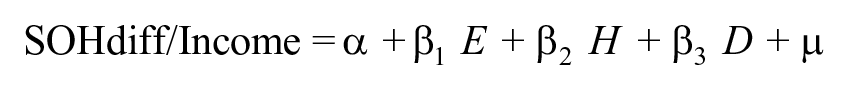
where SOHdiff/Income is the difference between the average market value and the average assessed value in each census block divided by the income of the census block, E is a vector of economic factors such as household permanent and current incomes that affect the value of homes in the census block, H is a vector of housing attributes such as the average age of the homes in the census block, and D is a vector of demographic variables that lead to different perceptions of the value of the homes in the census block, either by the market or by the local government property assessors, and μ is a random error term. We are interested in the demographic variables because we hypothesize that they may represent socioeconomic and racial differences in the way that homes are valued and assessed which may lead to horizontal inequities in the way the property tax is applied.

Our empirical model is similar to the one employed by Allen and Dare (2009). It regresses the market value shielded from taxation against several economic and demographic variables to determine which households receive the greatest amount of benefit from the SOH assessment cap. Our research explores several models, using different specifications of the dependent variable as well as different explanatory variables.

As mentioned, there is still debate among economists about whether property tax incidence should be measured relative to permanent or current income. Some argue that property tax incidence should be calculated using the home’s market value as a measure of permanent income because housing consumption decisions (and their accompanying tax burdens) are made over a long-term time horizon. Although this may be true, other economists question whether the property’s market value is really the best proxy for permanent income. Given the volatility of property market values during the inflationary period of the 1970s, and again during the housing boom and bust of the 2000s, it seems that market values are often based on factors that have nothing to do with permanent income. Furthermore, the political pressure that led to assessment caps was caused by the onerous burden of rising property assessments and their concurrent rising tax bills, which had to be paid out of current, not permanent, income. Thus, the opportunity cost of paying higher property taxes is current consumption, not house value (Englund 2003).

The arguments for using current income are compelling, but the preponderance of past studies have used permanent income proxied by the market value of the home as their measure for income. Therefore, as a compromise, this study estimates several regressions, some that use the average market value of the homes in the census block to measure permanent income, and some that use the median income of the census block to measure current income.

The data for this study were obtained from the Florida Department of Revenue and include the current market value and the assessed property value for all residential owner-occupied single-family detached residences located in the Jacksonville, FL Metropolitan Statistical Area (Clay, Duval, Nassau, and St. Johns counties) for the year 2019. The values of the variables were averaged at the census block level to calculate the current market value, the current assessed value and the difference between the market and assessed values per parcel in each of the census blocks in the four county MSA. These variables were then matched to census block data obtained from the US Census American Community Survey five-year estimates (2014–2018). Thus, property values were matched to a variety of demographic and socio-economic variables at the census block level. In cities, the block group is bounded by streets, roads, or creeks and is usually no bigger than one city block. However, in more rural areas, the block group is usually a larger area. Because this sample is restricted to owner-occupied detached residential units (as opposed to condominiums or rental units), the block group data provide a relatively accurate approximation of the homes and the homeowners in these small areas. There are obvious limitations to using block level data to approximate individual characteristics, but unfortunately, it is a necessity in studies that examine the characteristics of homeowners, since housing data do not include information on the owner’s characteristics. It gives us confidence to know that we are not the only researchers to do this. Data from these small homogenous block groups are routinely used as independent variables to estimate household characteristics by other researchers in the social sciences (see e.g., Chen, Glaeser, and Wessel 2019; Howell and Korver-Glenn 2021; Lee et al. 2019; Ruggles et al. 2019; Kang et al. 2021).

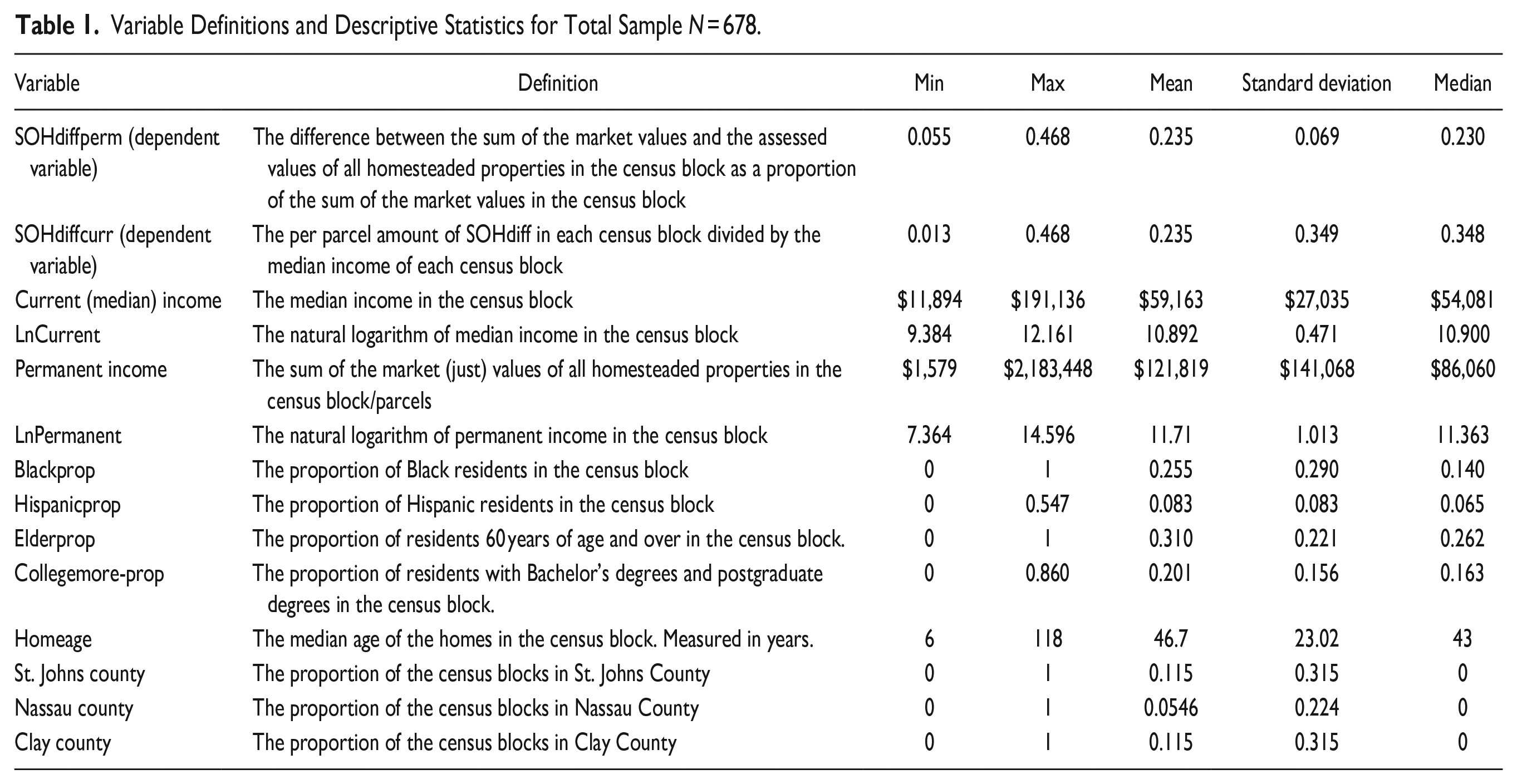
The description and the descriptive statistics for each variable used in the analysis are shown in Table 1. In Table 2, the descriptive statistics are broken down into the four counties in the sample. The bulk of the census blocks in the MSA are in Duval County which includes the urban core of the city and its surrounding environs. St. Johns, Clay, and Nassau counties contain primarily bedroom communities, retirement communities, and some rural lands. Baker County was excluded because its small sample size precluded any meaningful comparisons with the other counties, and it is primarily rural.

Table 1.

Variable Definitions and Descriptive Statistics for Total Sample N = 678.

Variable	Definition	Min	Max	Mean	Standard deviation	Median
SOHdiffperm (dependent variable)	The difference between the sum of the market values and the assessed values of all homesteaded properties in the census block as a proportion of the sum of the market values in the census block	0.055	0.468	0.235	0.069	0.230
SOHdiffcurr (dependent variable)	The per parcel amount of SOHdiff in each census block divided by the median income of each census block	0.013	0.468	0.235	0.349	0.348
Current (median) income	The median income in the census block	$11,894	$191,136	$59,163	$27,035	$54,081
LnCurrent	The natural logarithm of median income in the census block	9.384	12.161	10.892	0.471	10.900
Permanent income	The sum of the market (just) values of all homesteaded properties in the census block/parcels	$1,579	$2,183,448	$121,819	$141,068	$86,060
LnPermanent	The natural logarithm of permanent income in the census block	7.364	14.596	11.71	1.013	11.363
Blackprop	The proportion of Black residents in the census block	0	1	0.255	0.290	0.140
Hispanicprop	The proportion of Hispanic residents in the census block	0	0.547	0.083	0.083	0.065
Elderprop	The proportion of residents 60 years of age and over in the census block.	0	1	0.310	0.221	0.262
Collegemore-prop	The proportion of residents with Bachelor’s degrees and postgraduate degrees in the census block.	0	0.860	0.201	0.156	0.163
Homeage	The median age of the homes in the census block. Measured in years.	6	118	46.7	23.02	43
St. Johns county	The proportion of the census blocks in St. Johns County	0	1	0.115	0.315	0
Nassau county	The proportion of the census blocks in Nassau County	0	1	0.0546	0.224	0
Clay county	The proportion of the census blocks in Clay County	0	1	0.115	0.315	0

Table 2.

Descriptive Statistics for Each County.

Variable	Duval		St. Johns		Nassau		Clay
	n = 485		n = 78		n = 37		n = 78
	Mean	Median	Mean	Median	Mean	Median	Mean	Median
SOHdiff perm	0.240	0.23	0.201	0.193	0.220	0.515	0.220	0.225
SOHdiff curr	0.390	0.34	0.679	0.419	0.526	0.423	00.35	0.343
Medianinc	$55,983	$49,643	$65,255	$60,264	$103,742	$88,929	$63,121	$58,898
LnMedian-Inc	10.91	10.81	11.05	11.01	11.40	11.55	11.05	10.98
PermIncome	98,185	73,807	$225,574	$145,990	224,365	189,132	$104,996	$91,000
LnPermInc	11.49	11.21	11.91	11.89	12.32	12.15	11.56	11.42
Blackprop	0.29	0.19	0.053	0.016	0.04	0.02	0.08	0.04
Hispanic-prop	0.09	0.07	0.055	0.05	0.06	0.06	0.09	0.07
Elderprop	0.29	0.27	0.35	0.32	0.32	0.26	0.159	0.136
College-moreprop	0.185	0.14	0.32	0.32	0.371	0.372	0.158	0.136
Homeage	52	56	34.91	32	38.03	32.0	35.9	35

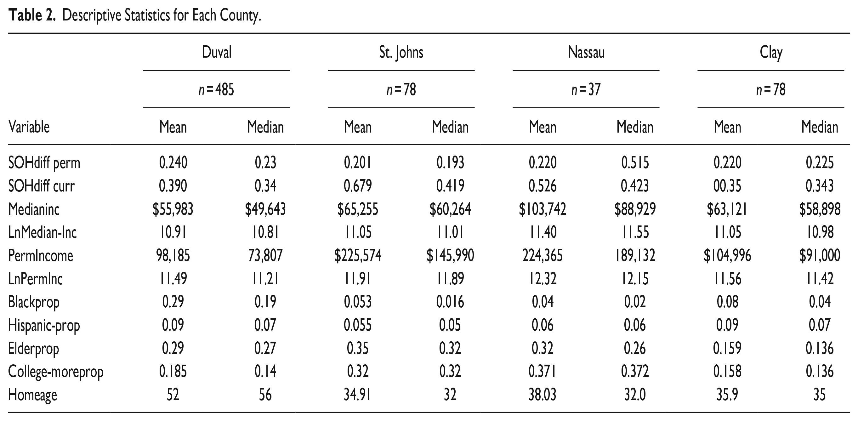
The means and medians of the variables by county show there are some meaningful differences in the counties. For example, the mean of the median income is higher in Nassau County than in the other three counties. Also, the values of the mean and median permanent income, which is the average market value of the homes in the census block, are higher in St. Johns and Nassau counties. Likewise, the proportions of older residents and well-educated residents are higher in St. Johns and Nassau Counties than in the other two counties. The proportions of Black residents in St. Johns, Nassau, and Clay Counties are much lower than in Duval County. This reflects the fact that Duval County is the urban center of the region. Even though the other three counties are suburban “bedroom communities,” they are not identical in character. For example, St. Johns and Nassau Counties contain relatively large enclaves of wealthy retirees, whereas Clay County has a large military presence and is more working class than St. Johns and Nassau. In addition, assessment practices in Florida are the sole responsibility of the county government, and so are likely to vary among the counties. For these reasons, we include dummy variables for each the counties in our regression models.

Although Duval County and its surrounding “bedroom community” counties are a specific example, it is important to note that they are representative of many large cities with surrounding suburban bedroom communities. The demographic statistics show that there has been considerable “White flight” to the surrounding suburbs relative to the central city of Jacksonville, which has occurred in almost all large cities in the United States. In addition, many of the demographic characteristics of the Jacksonville MSA are representative of other large metropolitan areas in the US. The Jacksonville MSA’s median household income in 2021 was $68,394 compared to the national median household income of $69,717 (US Census Bureau 2021). The Jacksonville MSA’s proportion of Black residents in 2020 was 0.208, which is very close to 0.204, the average Black proportion for the 50 urban areas with the highest Black populations in the US (Frey 2021). In addition, Florida home values are in the middle of the distribution of home values in the United States. According to Business Insider (Perino and Davis 2020), Florida’s median home price is ranked 25th out of the 50 states. Thus, although the results of this study are specific to the four counties in our sample, we believe they are generalizable to many other metropolitan areas in the United States.

Empirical Results: Vertical Equity

OLS regression analysis is employed (at the block group level) to estimate the impact of different socioeconomic characteristics on the market value shielded from taxation due to the Save Our Homes amendment. The models use two different representations of the dependent variable. The first is SOHdiffperm, which is the SOH difference as a proportion of the permanent income of the census block. It is calculated as the SOH difference per parcel in the census block divided by the average market value in the census block. The second dependent variable is SOHdiffcurr, which is the average SOH difference in the census block as a proportion of the current median income of the census block. It is calculated as the SOH difference per parcel divided by the median income in the census block.

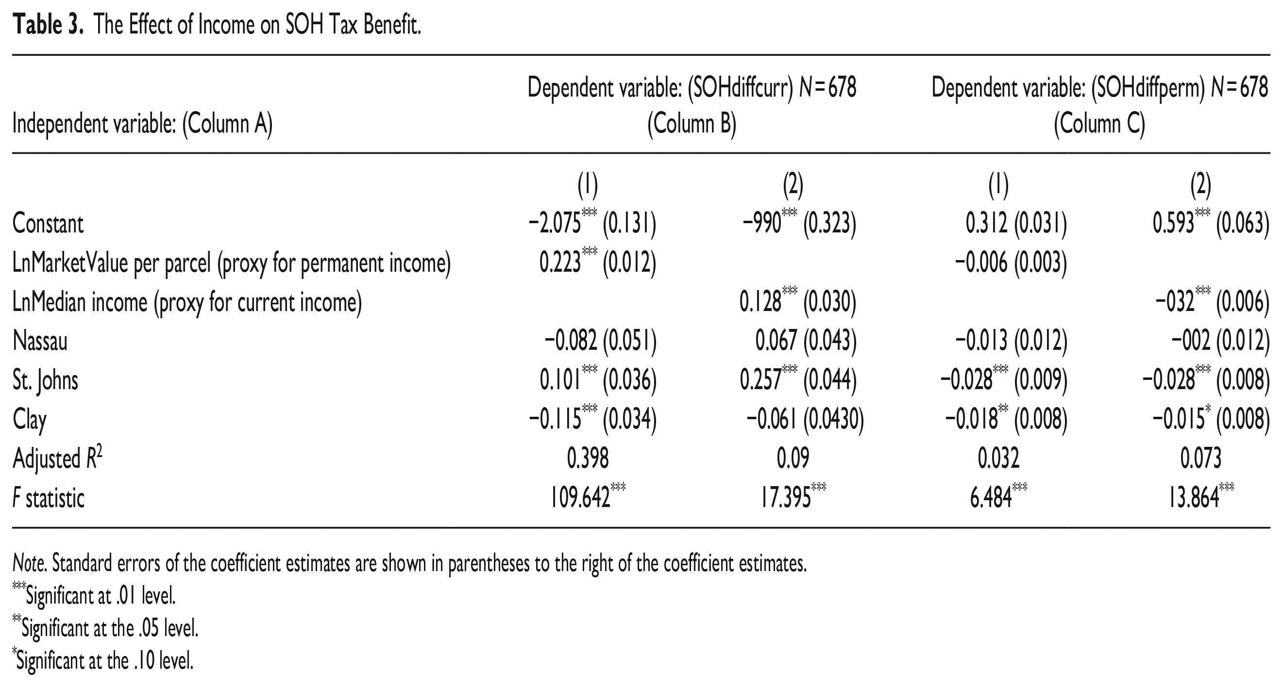
Table 3 shows the regression results for the model analyzing the effect of income alone on the SOH tax benefit. This is the traditional way that economists measure vertical equity. They examine the way the tax burden varies by income without controlling for other variables because vertical equity is defined as the distribution of the tax burden relative only to the distribution of income.¹ However, we have added dummy variables for the counties in the Jacksonville area to determine if the income effects differ among the counties. Column B in Table 3 shows the results when SOHdiffcurr is used as the dependent variable and Column C shows the results when SOHdiffperm is used as the dependent variable. In addition to the two different specifications of the dependent variable, we use two different specifications of the independent variable that measures income; one proxies permanent income (home value) and the other proxies current income (median income). Following Allen and Dare (2009), we use the natural logarithm of the income variables in the regression equations so that we can interpret the coefficients as the effect of a one percentage change in income on the dependent variable, which is the definition of income elasticity.

Table 3.

The Effect of Income on SOH Tax Benefit.

Independent variable: (Column A)	Dependent variable: (SOHdiffcurr) N = 678 (Column B)		Dependent variable: (SOHdiffperm) N = 678 (Column C)
	(1)	(2)	(1)	(2)
Constant	−2.075*** (0.131)	−990*** (0.323)	0.312 (0.031)	0.593*** (0.063)
LnMarketValue per parcel (proxy for permanent income)	0.223*** (0.012)		−0.006 (0.003)
LnMedian income (proxy for current income)		0.128*** (0.030)		−032*** (0.006)
Nassau	−0.082 (0.051)	0.067 (0.043)	−0.013 (0.012)	−002 (0.012)
St. Johns	0.101*** (0.036)	0.257*** (0.044)	−0.028*** (0.009)	−0.028*** (0.008)
Clay	−0.115*** (0.034)	−0.061 (0.0430)	−0.018** (0.008)	−0.015* (0.008)
Adjusted R²	0.398	0.09	0.032	0.073
F statistic	109.642***	17.395***	6.484***	13.864***

Note. Standard errors of the coefficient estimates are shown in parentheses to the right of the coefficient estimates.

***

Significant at .01 level.

Significant at the .05 level.

Significant at the .10 level.

Column B shows the results of the regression model when the dependent variable is the SOH benefit relative to the median income of the census block (SOHdiffcurr). Both the coefficient on permanent income (shown in column B1) and the coefficient on current income (shown in column B2) are positive and significant, which means the SOH benefit relative to current income increases as both the current and permanent income in the census block increases. In this case, the SOH benefit makes the property tax less equitable because the census blocks with higher current and permanent income will have a greater amount of their home’s value shielded from the property tax relative to their current incomes. The county dummy variables indicate there are significant differences in the way the SOH benefit is distributed in the counties. The dummy variable for St. Johns County indicates that the effect of both income measures on the SOH benefit relative to current income is larger in St. Johns County than in the other counties. This means the regressivity of the SOH benefit relative to current income is worse in St. Johns than in the other counties in our sample. Conversely, the negative and significant coefficient on the dummy variable for Clay County shown in column B1 indicates that increases in permanent income are less regressive in Clay County than in the other counties.

Column C shows the results of the regression model when the dependent variable is SOHdiffperm. The results in column C1 show that increases in permanent income have a significant negative effect on the benefits received from the SOH tax benefit relative to permanent income (SOHdiffperm), and column C2 shows that increases in current median income also have a significant negative effect on SOHdiffperm. This is good news for vertical equity because it shows that increases in both permanent and current income reduce the amount of SOH benefit homeowners receive relative to their homes’ market values. Since their SOH benefits are reduced, the effective property tax rate they pay will be greater. This makes the SOH benefit more vertically equitable. It is also interesting to note that the dummy variables for St. Johns and Clay counties are negative and significant. This means that the SOH benefit relative to permanent income decreases even more as both income measures rise in St. Johns and Clay counties relative to Duval and Nassau counties. Thus, the SOH benefit improves the vertical equity of the property tax even more in St. Johns and Clay counties than it does in Duval and Nassau counties.

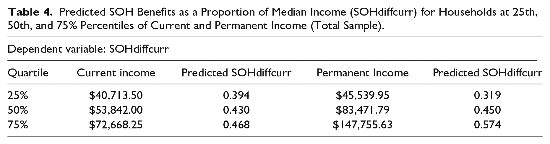
To understand the magnitude of the effects of changes in both permanent and current income on the SOH benefit relative to both income measures, we calculated the predicted SOH benefit as a proportion of permanent and current income for different quartiles of both income measures. These results are shown in Tables 4 and 5.

Table 4.

Predicted SOH Benefits as a Proportion of Median Income (SOHdiffcurr) for Households at 25th, 50th, and 75% Percentiles of Current and Permanent Income (Total Sample).

Dependent variable: SOHdiffcurr
Quartile	Current income	Predicted SOHdiffcurr	Permanent Income	Predicted SOHdiffcurr
25%	$40,713.50	0.394	$45,539.95	0.319
50%	$53,842.00	0.430	$83,471.79	0.450
75%	$72,668.25	0.468	$147,755.63	0.574

Table 5.

Predicted SOH Benefits as a Proportion of the Home’s Market Value (SOHdiffperm) for Households at the 25th, 50th, and 75% Percentiles of Current and Permanent Income (Total Sample).

Dependent variable: SOHdiffperm
Quartile	Current income	Predicted SOHdiffperm	Permanent income	Predicted SOHdiffperm
25%	$40,713.50	0.239	$45,539.95	0.236
50%	$53,842.00	0.230	$83,471.79	0.232
75%	$72,668.25	0.221	$147,755.63	0.229

Table 4 shows that the SOH benefit relative to current income (SOHdiffcurr) increases as both current and permanent incomes rise. This means that the SOH benefit makes the property tax less equitable with respect to current income. Homeowners in the census blocks at the 75th percentile of permanent income receive SOH benefits that are equal to over half (0.574) of the value of the median income in their census blocks. However, homeowners at the 25th percentile and 50th percentile of the permanent income distribution receive SOH benefits that are smaller proportions of the median income of their census blocks (0.319 and 0.450, respectively). Similar results are found when looking at the distribution of current income. The proportion of SOH benefits relative to the median income of the census block is almost half (0.468) for homeowners in the 75th percentile of the median income distribution but only 0.394 and 0.430, for the 25th and 50th percentiles, respectively. These differences demonstrate that the SOH benefit reduces the equity of the property tax relative to the current income of homeowners.

However, opposite results are found when the SOH benefit is compared to permanent income. The results in Table 5 show that the SOH benefit decreases as a proportion of permanent income (SOHdiffperm) as both current and permanent incomes rise. This means that the proportions of the benefit received relative to permanent income are slightly lower for the homeowners in the census blocks with higher median income and with higher average home market values. For example, the homeowners in the census blocks at the 75th percentile of the permanent income distribution get a proportion of SOH benefits relative to their homes’ market value of 0.229, and this is slightly lower than the proportions received by homeowners at the 25th percentile (0.236) and the 50th percentile (0.232). The same is true when the current (median) income of the census block rises. Homeowners in the census blocks at the 75th percentile of the distribution of median income have slightly lower proportions of SOH benefits relative to their permanent incomes (0.221) than the homeowners at the 25th or 50th percentiles (0.239 and 0.230, respectively.) This demonstrates that the SOH benefit improves the vertical equity of the property tax relative to the permanent income of the census block.

In summary, whether the Save Our Homes property tax benefit makes the property tax more or less equitable depends on which income measure is used in determining the ability to pay the tax. If policymakers use the traditional measure of the home’s market value as a proxy for permanent income, then the SOH benefit makes the property tax fairer, or at least it doesn’t harm its equity. However, if policymakers use current income as their measure of ability to pay, then the SOH benefit makes the property tax less fair. Relative to current income, the SOH benefit favors homeowners with higher levels of current income and higher home market values.

Empirical Results: Horizontal Equity

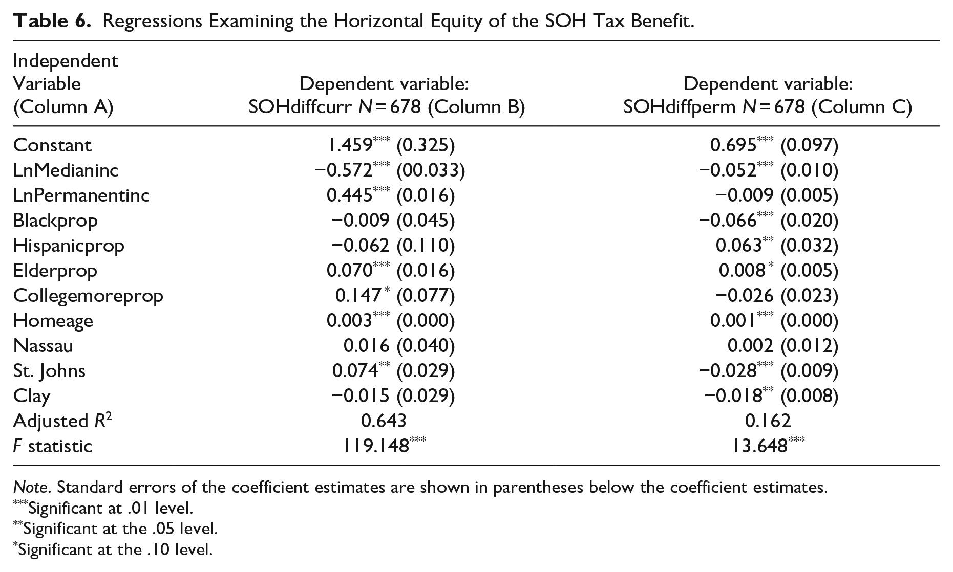
The next analysis examines if there are socio-economic or demographic characteristics that affect the distribution of the SOH tax benefit. If differences in the distribution of the SOH benefit based on these characteristics exist, then horizontal equity is violated. Table 6 shows the results of the horizontal equity regression models. As in the previous analysis, two different dependent variables are used in the regression models. Column B shows the results of the model that uses the SOH benefit as the proportion of the current median income of the census block (SOHdiffcurr) as the dependent variable, and column C shows the results using the SOH benefit as a proportion of the permanent income of the census block (SOHdiffperm) as the dependent variable. In both regressions, we include independent variables from the census block that denote current income, permanent income, race, ethnicity, education level, age of the homeowners, age of the home, and dummy variables that denote the county of residence. In this model, we include both the census block’s median income value (the current income proxy) and the average market value of the homes in the census block (the permanent income proxy) as independent variables. We include both income measures in these models to control for the confounding effect that current and permanent income may have on the other variables. However, since we included both income measures in the models, we examined the diagnostics for multicollinearity in our regression models to determine if the degree of multicollinearity was affecting the fit and interpretation of our models. We found no significant issues in this regard since none of the Variance Inflation Factors were greater than 3.5; thus, no adjustments were necessary.

Table 6.

Regressions Examining the Horizontal Equity of the SOH Tax Benefit.

Independent Variable (Column A)	Dependent variable: SOHdiffcurr N = 678 (Column B)	Dependent variable: SOHdiffperm N = 678 (Column C)
Constant	1.459*** (0.325)	0.695*** (0.097)
LnMedianinc	−0.572*** (00.033)	−0.052*** (0.010)
LnPermanentinc	0.445*** (0.016)	−0.009 (0.005)
Blackprop	−0.009 (0.045)	−0.066*** (0.020)
Hispanicprop	−0.062 (0.110)	0.063** (0.032)
Elderprop	0.070*** (0.016)	0.008 * (0.005)
Collegemoreprop	0.147 * (0.077)	−0.026 (0.023)
Homeage	0.003*** (0.000)	0.001*** (0.000)
Nassau	0.016 (0.040)	0.002 (0.012)
St. Johns	0.074** (0.029)	−0.028*** (0.009)
Clay	−0.015 (0.029)	−0.018** (0.008)
Adjusted R²	0.643	0.162
F statistic	119.148***	13.648***

Note. Standard errors of the coefficient estimates are shown in parentheses below the coefficient estimates.

***

Significant at .01 level.

Significant at the .05 level.

Significant at the .10 level.

The R² and F-statistic values are higher in the regression model that uses the SOH benefit as a proportion of current income (SOHdiffcurr) for the dependent variable than in the regression that uses the SOH benefit as a proportion of the permanent income (SOHdiffperm) for the dependent variable. However, both F-statistics are significantly different from zero. The difference in magnitude of these test statistics in the two models indicates that there is more variation that cannot be explained by the independent variables in the SOHdiffperm regression than in the SOHdiffcurr regression. However, this does not affect the interpretations of the significant variables. Therefore, the low R-squared values do not interfere with the interpretation of our significant results relative to individual explanatory variables.

Column B of Table 6 shows the regression results when the SOH benefit relative to current income (SOHdiffcurr) is used as the dependent variable. In this model the coefficient estimates of both income variables are significant although they have opposite signs. They indicate that the homes in the census blocks with higher median incomes have lower SOH benefits as a proportion of current income, but homes in the census blocks with higher home market values (permanent income) have higher SOH benefits as a proportion of current income. These were the same results found when each income variable was entered by itself into the regression model (the results shown in Table 3). However, in this model, we are controlling for the confounding effects that other socio-demographic variables correlated with income may have on the true income effect. Thus, the income effects in the first model were not serving as a stand-in for the effect of other socio-demographic variables that are correlated with income. We can unequivocally say that whether the SOH benefit improves or harms the vertical equity of the property tax depends on the income measure (permanent or current) that is used as the standard for the ability to pay the tax.

The other significant variables in the model indicate there are horizontal inequities in the SOH benefit relative to current income. For example, the homeowners in census blocks that contain older homes and older residents receive SOH benefits relative to current income that are significantly higher than those in the census blocks with newer homes and younger residents. This is not surprising since older homes and older residents have had more time to accumulate SOH benefits as the market value of their homes grow but the assessed values are limited to 3% or less per year. Also, the census blocks with higher proportions of well-educated residents receive greater SOH benefits as a proportion of current income than the census blocks with lower levels of educational attainment.

Another horizontal inequity is caused by the county in which the homes reside. Holding all other things equal, homes in St. Johns County receive more SOH benefits relative to their current incomes than identical homes in the other counties in the Jacksonville MSA. We’re not sure why this is the case, except that property appraisals for tax purposes are the province of each county so the training of appraisers is likely to vary.

A very important finding in this model is that there are no significant racial differences in the amount of SOH benefits received relative to the current income of the census block. Neither of the coefficient estimates of the variables indicating the proportions of Blacks or Hispanics in the census blocks are significantly different from zero in this model. As we will see shortly, this is not the case in the next model.

Column C of Table 6 shows the regression results when the SOH benefit relative to permanent income (SOHdiffperm) is used as the dependent variable. These results indicate that the median income of the census block has a negative and significant effect on the SOH benefit as a proportion of permanent income, which is good news for vertical equity. Homes in the census blocks with higher median incomes receive less benefit from the SOH assessment cap and so will pay a higher effective property tax rate relative to their homes’ values. The permanent income variable in this model has no significant effect on the SOH benefit relative to permanent income (SOHdiffperm), so it does not affect vertical equity either positively or negatively. Note that the income effects in this model are the same as those in the model that included income by itself (Table 3, Column C1). Thus, once again, the income effects in the first model were not serving as a stand-in for the effect of other socio-demographic variables that are correlated with income.

The results in Table 6, Column C show there are horizontal inequities in the SOH benefits received relative to the permanent income (SOHdiffperm) of the census block. As was the case when the dependent variable was SOH benefits relative to current income (SOHdiffcurr), the variables representing older homes and older residents are positive and significant. This means the SOH benefits relative to permanent income are significantly higher than those in the census blocks with newer homes and younger residents. Once again, this is most likely due to the accumulation of SOH benefits over time. Also, as was the case in the results reported in Column A, there are significant differences in the SOH benefits in the different counties. In this model, the homes in St. Johns County and Clay County receive significantly less SOH Benefit relative to permanent income than homes in Duval or Nassau Counties, other things equal.

However, the most serious horizontal inequity is implied by the negative and significant effect of the variable representing the proportion of Blacks residing in the census block. This means that the SOH benefit as a proportion of permanent income decreases as the proportion of Blacks in the census block increases. This effect cannot be blamed on the statistical fact that Blacks tend to have lower levels of education and income than their White counterparts because income and education are included in the equation as control variables. Unfortunately, this racial effect is quite large, and it is made even more serious by the degree of racial segregation in the study area. The stark differences in the racial makeup among the counties are shown in Figure 1. The census blocks with a greater representation of racial minorities are shown on the map in darker shades. This contrasts significantly with the graph in Figure 2 that shows the geographical distribution of the greatest SOH benefits as a proportion of permanent income (SOHdiffperm), also shown in the darker shades. Except for a few census blocks in Duval County that are located on the St. Johns River or the Atlantic Ocean, the darker shaded census blocks showing the greatest SOH benefits are in the suburban counties, especially St. Johns and Nassau counties. In fact, the two maps are almost mirror images of one another. The dark shaded areas in the first map showing the largest proportion of minorities in the MSA are the light shaded areas in the second map showing the least amount of SOH benefit as a proportion of the home’s market value.

Figure 1.

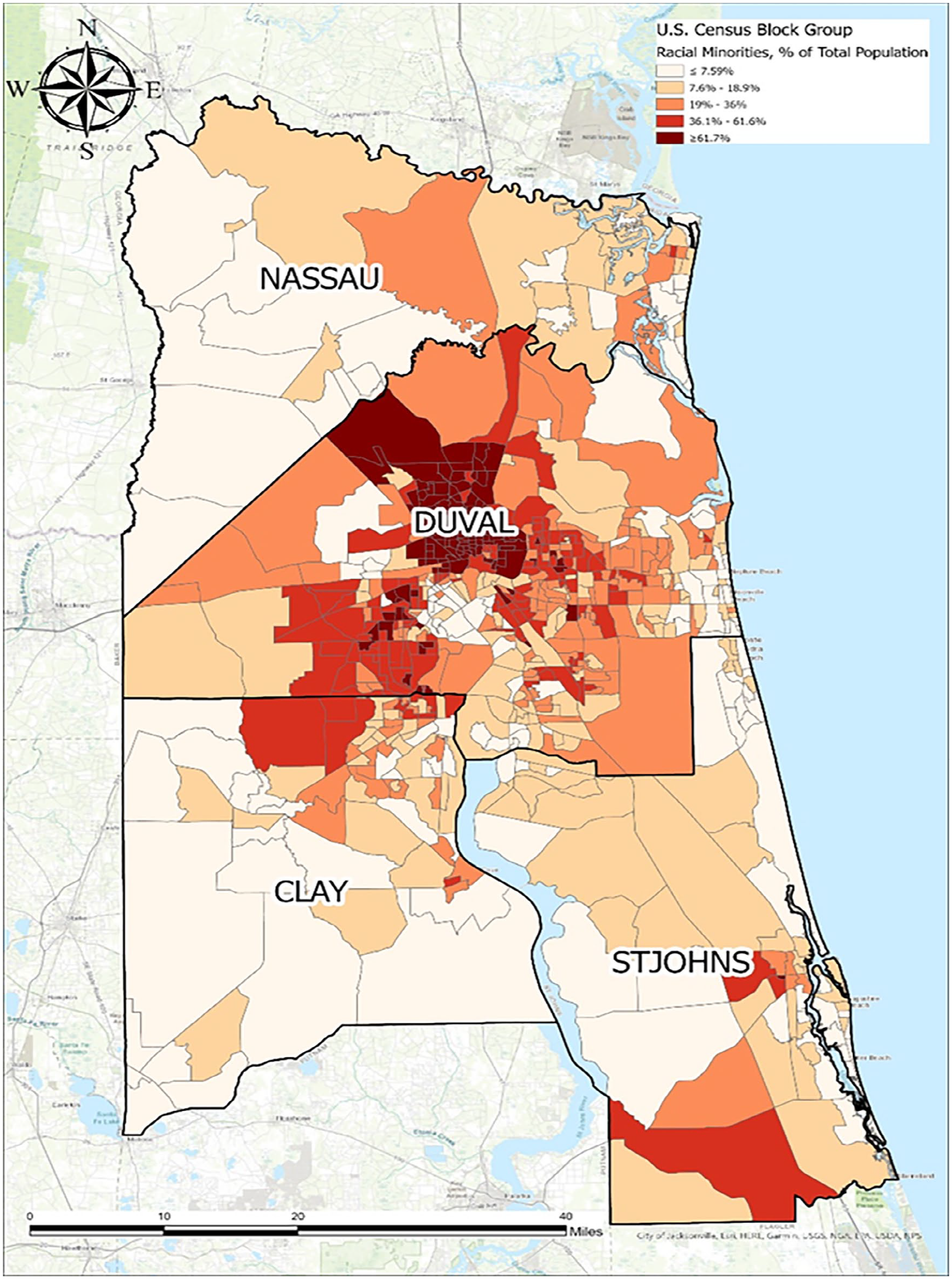
Map created by Robert Jordan.

Figure 2.

SOH value as a proportion of the home’s value in the study area.

Map created by Robert Jordan

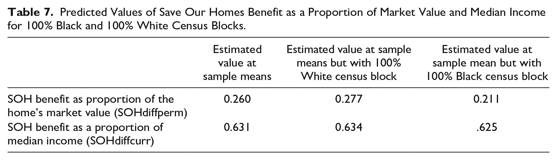
There are 11 census blocks in our sample that are 100% Black, and 95 that are 100% White. To explore the difference between the SOH benefits in these census blocks, we used the regression models to estimate SOHdiffperm and SOHdiffcurr when the means of the explanatory variables in the total sample were inserted into the regression equation. Then we repeated this analysis with the sample means but with the Black variable equal to 1, to indicate a 100% Black census block, and again with the Black variable equal to 0 to indicate a 100% White census block. The results of this analysis are shown in Table 7. Homeowners can expect to receive a SOH benefit equal to 26% of the average value of the homes in the census block and 63.1% of the value of the median income in the census block, when the mean values of all explanatory variables are entered into the regression equations. In contrast, if the sample average home were in a 100% Black census block, then the homeowners would receive only 21.1% of the average value of the homes in the census block and 62.5% of the value of the median income in the census block. But if the sample average home were in a 100% White census block, the benefits would be higher than the average for the total sample: 27.7% of the value of the average home value in the census block, and 63.4% of the value of the median income in the census block. Thus, homes in 100% Black census blocks receive, on average, 6.6 percentage points less value (27.7%–21.1%) from the SOH benefit relative to their home’s value.

Table 7.

Predicted Values of Save Our Homes Benefit as a Proportion of Market Value and Median Income for 100% Black and 100% White Census Blocks.

	Estimated value at sample means	Estimated value at sample means but with 100% White census block	Estimated value at sample mean but with 100% Black census block
SOH benefit as proportion of the home’s market value (SOHdiffperm)	0.260	0.277	0.211
SOH benefit as a proportion of median income (SOHdiffcurr)	0.631	0.634	.625

Our results are consistent with recent research done by others, especially Beal, Borg, and Stranahan (2016, 2017) that examined the same geographic area. However, these results are not specific to just one part of the country. Howard and Avenancio-León (2022) used over a decade of tax assessment and sales data for 118 million homes throughout the country. They found that property tax assessments were higher relative to the sales values of the homes in areas with more Black residents. Berry (2021) examined assessment to sales ratios using Census Housing Values in Chicago, New York, Detroit, and New Orleans. He found that the relative assessment ratio, which is the property’s assessment to sales ratio divided by the county average assessment to sales ratio was under one for census tracts with 0%–20% Black residents, but the ratio increased steadily as the percentage of Black residents in the census tract increased, so that when the census tract reached 90%–100% Black residents the ratio was close to 1.6. This means that the census tracts with 20% or fewer Black residents had assessment/sales ratios that were below the county average, but the census tracts that had 90%–100% Black residents had assessment/sales ratios that were 60% over the county average. This either means that county governments’ property appraisers are overvaluing the homes in predominantly Black neighborhoods for tax purposes, or the private sector residential property appraisers are undervaluing the homes’ market values in predominantly Black neighborhoods, or most likely, some of both. For purposes of our study, this means that the differences between the market values and the assessed values of the homes in predominantly Black census blocks are smaller, so they receive significantly less benefit from the Save Our Homes tax break and pay relatively more property tax relative to their homes’ market values than the homes in predominately White neighborhoods.

Studies such as ours are important because think tanks and the popular media are paying attention to this problem (Kamin 2020; Mock 2020, 2021; Narragon et al. 2021; Van Dam 2020). For example, a recent report from the Brookings Institution (Perry et al. 2018) concluded that similar homes with similar amenities in majority Black neighborhoods were worth 23% less, on average, than homes in neighborhoods with very few or no Black residents. Interestingly, this is almost the same percentage difference that we found in our study.² They estimated that this difference amounted to $156 billion in cumulative losses in majority Black neighborhoods. Not only do differences such as these result in property tax inequities, but they also affect the amount of home equity that Black homeowners have available for home renovations, children’s college expenses, and down payments when they are ready to move to their next home.

Discussion

As stated in the beginning of the paper, this study was designed to answer two questions: (1) Do assessment caps make the property tax more regressive (or less progressive), and (2) Are they fair to all taxpayers, or do some demographic and socioeconomic groups get more benefit from the caps than others? The answer to the first question depends on the income measure used to determine the property owner’s ability to pay the tax. Using the traditional income measure of the home’s market value as a proxy for permanent income, the answer is no, the property tax caps do not make the property tax more regressive. When we analyzed the relationship between both current and permanent income and the SOH benefit as a proportion of the home’s market value (SOHdiffperm), we found that the benefit relative to the home’s value was smaller in the census blocks that had higher home values and higher median incomes. Thus, we concluded that the SOH assessment cap makes the property tax slightly less regressive (or more progressive) relative to the market value of the home. This result was surprising based on previous research that found that assessment caps made the property tax more regressive (Anderson 2006; Bowman 2006; Dye, McMillen, and Merriman 2006; IAAO 2008; Moore 2008).

However, the answer to whether the assessment cap makes the property tax more regressive is yes when the current income (proxied by the median income of the census block) is used to measure the homeowner’s ability to pay the property tax. When we analyze the relationship between both current and permanent income on the SOH benefit as a proportion of the median income of the census block (SOHdiffcurr), we find that the benefit relative to current income is larger in the census blocks that have higher median incomes and higher home values. Thus, the SOH assessment cap makes the property tax more regressive (or less progressive) relative to the homeowner’s current income with respect to both current and permanent income. This is important because it is current income that is forgone when homeowners pay their property taxes.

Since property tax assessment caps are regressive relative to current income, more equitable forms of property tax relief should be considered. For example, Florida already has a Homestead Exemption that exempts the first $25,000 of a home’s assessed value if the home is owner-occupied and valued at $50,000 or less. The homestead exemption is $50,000 if the home is valued at $75,000 or more. This is more equitable than the SOH tax break because the exemption is a greater percentage of the home’s value for lower valued homes. However, the counties with the lowest property values often must increase their millage rates to have enough revenues to cover their county expenditures. This reduces the tax relief and the equity of the property tax for homeowners whose home values are above $75,000. Thus, a policy with progressive millage rates combined with the homestead exemption would be the most equitable form of property tax relief.

The answer to the second question is a resounding no, the assessment caps are not fair to all taxpayers. There are some groups that get more benefit from the caps than others. Our research finds that assessment caps cause serious horizontal inequities, especially relative to the racial distribution of the census blocks where the homes are located. The 100% Black census blocks in our sample received 6.6 percentage points less value from the caps relative to the market values of their homes than the 100% White census blocks. Differences like these mean that homeowners in 100% Black neighborhoods pay more property tax relative to the value of their homes than comparable homeowners in 100% White neighborhoods. These results are consistent with previous studies that found higher assessment to sales (A/S) ratios in neighborhoods with higher percentages of minorities (Allen and Dare, 2009; Avenancio-León 2022; Berry 2021; Harris 2004; Howell and Korver-Glenn, 2021).

Our results are especially troubling because this study controls for income and education levels, two variables that are correlated with race. In other studies that have not controlled for these variables, racial differences in A/S ratios are often attributed to differences in income and education levels between minorities and Whites. However, in this study, racial differences in the benefits of assessment caps persist despite these variables being controlled in the analysis. Our research was conducted in one large urban/suburban metropolitan area in the south. But other recent studies (Howard and Avenancio-León 2022; Berry 2021) have shown that these differences in property assessments in Black and White neighborhoods exist in many other areas of the United States. We believe our findings are not an isolated case. Horizontal inequities such as these need to be addressed by property appraisers and policy makers.

As stated above, the problem seems to be two-fold: county government property appraisers over-value the homes in predominantly Black neighborhoods for tax purposes, and private sector property appraisers under-value the market value of homes in predominantly Black neighborhoods. This means that the difference between a home’s market value and assessed value is smaller in predominantly Black neighborhoods; thus, homeowners in predominately Black neighborhoods pay a higher effective property tax rate than comparable homeowners in predominantly White neighborhoods. Since the problem originates with property appraisers, it can be addressed with better training for property appraisers. Government property appraisers need to be made aware of the differences in home values that exist among the various neighborhoods of their county. A three bedroom, two bath, 1,800 square feet home does not sell for the same price in every neighborhood of the county. Every home buyer knows this, so it needs to be acknowledged by the county’s property appraisers using large data sets available from real estate sites such as Zillow.com and Realtor.com to finetune their appraisals in different parts of the county.

Real estate agents and private sector property appraisers also need to be trained to identify their own implicit, even unconscious, racial biases. One egregious example of a biased private sector property appraisal occurred in our sample area in 2020 (Kamin 2020). A bi-racial couple had their home in a predominantly White neighborhood appraised to refinance it. The Black spouse was home for the appraisal. When the appraisal came back low, they scheduled a second appraisal. In preparation for the second appraisal, they removed all the family photos, and art and books that featured Blacks, and the White spouse was home when the appraiser came. The new appraisal came back 41% higher. Unfortunately, examples like this are still common in all parts of the country. But even more important than training White property appraisers to recognize and correct their racial biases, the property appraisal field needs to diversify. According to the U.S. Bureau of Labor Statistics (2022), over 95% of property appraisers are White. Extensive recruitment for people of color must be made by educational institutions that train property appraisers and by the Appraisal Institute.

We all hope to live in a color-blind society someday, but research such as ours, shows that our society is not quite there yet. Until it is, research that points out racial disparities, and policy makers that devise solutions to overcome the inequities created by the disparities are vitally important. This research is an attempt to contribute to these efforts.

Footnotes

Acknowledgements

The authors wish to thank Robert Jordan for compiling the data and creating the maps for this project.

Declaration of Conflicting Interests

The author(s) declared no potential conflicts of interest with respect to the research, authorship, and/or publication of this article.

Funding

The author(s) received no financial support for the research, authorship, and/or publication of this article.

ORCID iD

Mary O. Borg

Notes

Author Biographies

Mary O. Borg is a Professor of Political Economy at the University of North Florida. Her research interests include the economic consequences of state lotteries, lottery-funded merit scholarships, and other public sector policy issues. Her publications have appeared in the National Tax Journal, Public Finance Review, and the Journal of Economic Education.

John Rody Borg is a Professor of Economics and Public Policy at Jacksonville University. His research interests include the market valuation of mergers in the early twentieth century, the economic consequences of Florida merit scholarships, education pedagogy and other public sector policy issues. His publications have appeared in the International Journal of Industrial Organization, the Journal of Financial and Quantitative Analysis, Florida Political Chronicle and College Teaching. He works as an expert economist and has testified on economic damages in state and federal courts over 100 times.

References

Aaron

Henry

. 1974. “A New View of Property Tax Incidence.” The American Economic Review 64 (2): 212–21.

Allen

Marcus

. 2003. “Measuring Vertical Property Tax Inequity in Multifamily Property Markets.” Journal of Real Estate Research 25 (2): 171–84. doi:10.1080/10835547.2003.12091107

Allen

Marcus

Dare

William

. 2002. “Identifying Determinants of Horizontal Property Tax Inequity: Evidence From Florida.” Journal of Real Estate Research 24 (2): 153–64. doi:10.1080/10835547.2002.12091091

Allen

Marcus

Dare

William

. 2009. “Changes in property tax progressivity for Florida homeowners after the ‘Save Our Homes amendment.’” Journal of Real Estate Research 31 (1): 81–92. doi:10.1080/10835547.2009.12091232

Anderson

Nathan B.

2006. “Property Tax Limitations: An Interpretative Review.” National Tax Journal 59 (3): 685–94. doi:10.17310/ntj.2006.3.18

Avenancio-León

Carlos F.

Howard

Troup

. 2022. “The Assessment Gap: Racial Inequalities in Property Taxation.” The Quarterly Journal of Economics 137 (3): 1383–434.

Baer

David

. 2007

“State and Local Property Tax Burdens in 2005.”

AARP, May 1. https://www.aarp.org/money/taxes/info-2007/2007-09-tax.html

Beal-Hodges

Mary

Borg

Mary O.

Stranahan

Harriet A.

2016. “A re-examination of the property tax burden.” Journal of Business & Economics Research 14 (2): 51–60.

Beal

Mary

Borg

Mary O.

Stranahan

Harriet

. 2017. “The Equity Effects of Property Tax Caps: Evidence From Florida.” Academic Journal of Interdisciplinary Studies 6 (s2): 141–51. doi:10.2478/ajis-2018-0039

10.

Berry

Christopher R.

2021. “Reassessing the Property Tax.” SSRN, March 9. https://papers.ssrn.com/sol3/papers.cfm?abstract_id=3800536

11.

Bidanset

Paul

McCord

Michael

Davis

Peadar

Sunderman

Mark

. 2019. “An Exploratory Approach for Enhancing Vertical and Horizontal Equity Tests for Ad Valorem Property Tax Valuations Using Geographically Weighted Regression.” Journal of Financial Management of Property and Construction 24 (2): 231–50. doi:10.1108/jfmpc-04-2019-0033

12.

Birch

John W.

Sunderman

Mark A.

Smith

Brent C

. 2004. “Vertical Inequity in Property Taxation: A Neighborhood Based Analysis.” The Journal of Real Estate Finance and Economics 29 (1): 71–8. doi:10.1023/b:real.0000027201.39235.63

13.

Bowman

John H.

2006. “Property Tax Policy Responses to Rapidly Rising Home Values: District of Columbia, Maryland, and Virginia.” National Tax Journal 59 (3): 717–33. doi:10.17310/ntj.2006.3.21

14.

Bowman

John H.

Mikesell

John L.

1975. “Uniform Assessment of Property: Returns From Institutional Remedies.” National Tax Journal 31 (2): 137–52. doi:10.1086/ntj41863106

15.

Bowman

John H.

Mikesell

John L.

1989. “Elected Versus Appointed Assessors and the Achievement of Assessment Uniformity.” National Tax Journal 42 (2): 181–9. doi: 10.1086/NTJ41788787

16.

Cammenga

Janelle

. 2021. “Where Do People Pay the Most in Property Tax.” Tax Foundation, September 1. https://taxfoundation.org/county-property-tax-paid-2021/

17.

Case

Karl E.

1978. Property Taxation: The Need for Reform. Cambridge, MA: Ballinger. https://www.proquest.com/books/property-taxation-need-reform-united-states/docview/59054503/se-2?accountid=14690

18.

Chen

Jiafeng

Glaeser

Edward L.

Wessel

David

. 2019. “The (non-) Effect of Opportunity Zones on Housing Prices.” No. w26587. National Bureau of Economic Research.

19.

Cornia

Gary

Slade

Barrett A.

2005. “Property Taxation of Multifamily Housing: An Empirical Analysis of Vertical and Horizontal Equity.” Journal of Real Estate Research 27 (1): 17–46. doi:10.1080/10835547.2005.12091152

20.

Cornia

Gary

Slade

Barrett A.

2006. “Horizontal Inequity in the Property Taxation of Apartment, Industrial, Office, and Retail Properties.” National Tax Journal 59 (1): 33–55. doi:10.17310/ntj.2006.1.02

21.

Dye

Richard F.

McMillen

Daniel P.

Merriman

David F.

(2006). “Illinois’ Response to Rising Residential Property Values: An Assessment Growth Cap in Cook County.” National Tax Journal 59 (3): 707–16. doi:10.17310/ntj.2006.3.20.

22.

Englund

. (2003). Taxing Residential Housing Capital. Urban Studies 40(5–6): 937–952. https://doi.org/10.1080/0042098032000074254

23.

Florida Department of Revenue. 2020. “County just, Assessed, and Taxable Value.” https://floridarevenue.com/property/Documents/jat.pdf (accessed April 29, 2021).

24.

Frey

W. H.

2021. “Mapping America’s Diversity With the 2020 Census.” Brookings. January 29, 2023.

25.

Goolsby

William

. 1997. “Assessment Error in the Valuation of Owner-Occupied Housing.” Journal of Real Estate Research 13 (1): 33–45. doi:10.1080/10835547.1997.12090863.

26.

Harris

Lee A.

2004. “Assessing Discrimination: The Influence of Race in Residential Property Tax Assessments.” Journal of Land Use 20 (1): 1-60.

27.

Hodge

Timothy R.

McMillen

Daniel P.

Sands

Gary

Skidmore

Mark

. 2017. “Assessment Inequity in a Declining Housing Market: The Case of Detroit.” Real Estate Economics 45 (2): 237–58.

28.

Howell

Junia

Korver-Glenn

Elizabeth

. 2021. “The Increasing Effect of Neighborhood Racial Composition on Housing Values, 1980–2015.” Social Problems 68 (4): 1051–71.

29.

IAAO (International Association of Assessing Officers) 2008. “Assessed Value Cap Overview.” Journal of Property Tax Assessment and Administration 7 (1): 57–67.

30.

Kamin

Debra

. 2020. “Black Homeowners Face Discrimination in Appraisals.” New York Times. August 25. https://www.nytimes.com/2020/08/25/realestate/blacks-minorities-appraisals-discrimination.html

31.

Kang

Yuhao

Zhang

Fan

Peng

Wenzhe

Gao

Song

Rao

Jinmeng

Duarte

Fabio

Ratti

Carlo

. 2021

“Understanding House Price Appreciation Using Multi-source Big Geo-data and Machine Learning.”

Land Use Policy 111:104919.

32.

Lee

Barrett A.

Farrell

Chad R.

Reardon

Sean F.

Matthews

Stephen A.

2019. “From Census Tracts to Local Environments: An egocentric Approach to Neighborhood Racial Change.” Spatial Demography 7: 1–26. doi:10.1007/s40980-018-0044-5

33.

McGreal

Stanley

Brown

Louise

Adair

Alastair

Webb

James

. 2007. “Vertical Tax Equity: An Analysis of Residential Valuation in a Major U.K. City.” Journal of Housing Research 16 (1): 1–18. doi:10.1080/10835547.2007.12091973

34.

McMillen

Daniel

Singh

Ruchi

. 2020. “Assessment Regressivity and Property Taxation.” The Journal of Real Estate Finance and Economics 60: 155–69.

35.

Metcalf

Gilbert

. 1993. “The Lifetime Incidence of State and Local Taxes: Measuring Changes During the 1980s.” doi:10.3386/w4252

36.

Mieszkowski

Peter M.

1967. “On the Theory of Tax Incidence.” Journal of Political Economy 75 (3): 250–62.

37.

Mock

Brentin

. 2020. “A Neighborhood’s Race Affects Home Values More Now Than in 1980.” Bloomberg. September 21. https://www.bloomberg.com/news/articles/2020-09-21/race-gap-in-home-appraisals-has-doubled-since-1980

38.

Mock

Brentin

. 2021. “What it Will Take to Close the Race Gap in Home Appraisal.” Bloomberg. March 3. https://www.bloomberg.com/news/articles/2021-03-03/appraisers-acknowledge-bias-in-home-valuations

39.

Moore

J. Wayne

. 2008. “Property Tax Equity Implications of Assessment Capping and Homestead Exemptions for Owner-Occupied Single-Family Housing.” Journal of Property Tax Assessment & Administration 5 (3): 37–72. https://www.proquest.com/scholarly-journals/property-tax-equity-implications-assessment/docview/210712848/se-2?accountid=14690

40.

Musgrave

Richard A.

1961. The Theory of Public Finance: A Study in Public Economy. New York, NY: McGraw-Hill.

41.

Narragon

Melissa

Wiley

Danny

McManus

Doug

Vivian

Kangli

Xue

Karamon.

Kadiri

2021. “Racial and Ethnic Valuation Gaps in Home Purchase Appraisals.” Freddie Mac Economic & Housing Research Note 9 (20): 2021.

42.

Perino

Marissa

Davis

Dominic-Madori

. 2020. “Here’s the Typical Home Price in Every State — and What You Can Actually Get for That Money.” Business Insider. April 10.

43.

Perry

Andre

Rothwell

Jonathan

Harshbarger

David

. 2018. “The Devaluation of Assets in Black Neighborhoods.” Library Catalog: www.brookings.edu

44.

Phares

Donald

. 1980. Who Pays State and Local Taxes? Cambridge, MA: Oelgeschlager, Gunn and Hain.

45.

Plummer

Elizabeth

. 2003. “Evidence on the Incidence of Residential Property Taxes Across Households.” National Tax Journal 56 (4): 739–53. doi:10.17310/ntj.2003.4.02

46.

Ruggles

Fitch

Magnuson

Schroeder

. (2019, May). Differential privacy and census data: Implications for social and economic research. In AEA papers and proceedings (Vol. 109, pp. 403-408). 2014 Broadway, Suite 305, Nashville, TN 37203: American Economic Association.

47.

Sirmans

G. Stacy

Diskin

Barry A.

Friday

H. Swiny

. 1995. “Vertical Inequity in the Taxation of Real Property.” National Tax Journal 48 (1): 71–84. doi:10.1086/ntj41789124

48.

Skidmore

Mark

Ballard

Charles L.

Hodge

Timothy R.

2010. “Property Value Assessment Growth Limits and Redistribution of Property Tax Payments: Evidence From Michigan.” National Tax Journal 63 (3): 509–37.

49.

smartasset.com. 2021. “Florida Property Tax Calculator.” SmartAsset. https://smartasset.com/taxes/florida-property-tax-calculator (accessed August 30, 2021).

50.

Smith

Brent

. 2000. “Applying Models for Vertical Inequity in the Property Tax to a Non-Market Value State.” Journal of Real Estate Research 19 (3): 321–44. doi:10.1080/10835547.2000.12091019

51.

Stiglitz

Joseph E.

Rosengard

Jay K.

2015. Economics of the Public Sector. New York, NY: Norton.

52.

Suits

Daniel B.

1977

“Measurement of Tax Progressivity.”

The American Economic Review 67 (4): 747–52. http://www.jstor.org/stable/1813408

53.

Sunderman

Mark

Birch

John

Cannaday

Roger

Hamilton

Thomas

. 1990. “Testing for Vertical Inequity in Property Tax Systems.” Journal of Real Estate Research 5 (3): 319–34. doi:10.1080/10835547.1990.12090625

54.

Tiebout

Charles M.

1956. “A Pure Theory of Local Expenditures.” Journal of Political Economy 64 (5): 416–24.

55.

U.S. Bureau of Labor Statistics. 2022. “Household Data Annual Averages. Table 11. Employed Persons by Detailed Occupation, Sex, Race, and Hispanic or Latino Ethnicity Employed Persons.” https://www.bls.gov/cps/cpsaat11.htm

56.

US Census Bureau. 2021. “American Community Survey 1-Year Estimates.” Census Reporter Profile page for Jacksonville, FL Metro Area. http://censusreporter.org/profiles/31000US27260-jacksonville-fl-metro-area.

57.

Van Dam

Andrew

. 2020. “Black Families Pay Significantly Higher Property Taxes Than White Families, New Analysis Shows.” Washington Post. July 2. https://www.washingtonpost.com/business/2020/07/02/black-property-tax/

58.

Walczak

Jared

. 2020. “Property Tax Limitation Regimes: A Primer.” Tax Foundation, June 16. https://taxfoundation.org/property-tax-limitation-regimes-primer/

59.

Zodrow

George R.

2001. “The Property Tax as a Capital Tax: A Room With Three Views.” National Tax Journal 54 (1): 139–56.