Modeling dynamic processes with panel data: An application of continuous time models to prevention research

Abstract

Many interventions are characterized by repeated observations on the same individuals (e.g., baseline, mid-intervention, two to three post-intervention observations), which offer the opportunity to consider differences in how individuals vary over time. Effective interventions may not be limited to changing means, but instead may also include changes to how variables affect each other over time. Continuous time models offer the opportunity to specify differing underlying processes for how individuals change from one time to the next, such as whether it is the level or change in a variable that is related to changes in an outcome of interest. After introducing continuous time models, we show how different processes can produce different expected covariance matrices. Thus, models representing differing underlying processes can be compared, even with a relatively small number of repeated observations. A substantive example comparing models that imply different underlying continuous time processes will be fit using panel data, with parameters reflecting differences in dynamics between control and intervention groups.

Keywords

Continuous time models differential equations stochastic perturbations dynamical systems latent change score model integration of structural-differential equations

Intervention research often focuses on the identification of mean differences as the primary outcome of interest. We proceed from developmental and clinical perspectives built on dynamic systems theory, where interventions may result in not only mean-level changes but also changes in the relations within and between variables over time (Compas et al., 2015; Horowitz et al., 2007; Shelleby et al., 2018). That is, by understanding and modifying the underlying processes that contribute to increased risk and dysfunctional outcomes, it may be possible to promote desirable outcomes over time.

To understand the covariance between variables and within variables as they change across time, repeated observations are required. Many intervention studies involve collecting repeated observations on the same individuals (e.g., baseline, mid-intervention, two to three post-intervention observations), which offer the opportunity to test for differences in how individuals or groups vary over time. Moreover, effective interventions may not be limited to changing the mean levels of outcomes; they may also change how variables relate to each other. Indeed, changing relations between variables may be one of the fundamental differences between interventions that have enduring effects and those that do not, as this would be suggestive of a change in the dynamics of an individual’s system. The present article focuses on providing tools for modeling concurrent change between variables to offer prevention science the opportunity to address novel questions about concurrent change and to model changes in dynamics, even with a limited number of repeated observations.

The initial sections of this article provide a grounding in language for expressing change relations and then explore the effects and challenges of external influences on the modeling of change. The fitting of models for repeated observations that exhibit frequent reciprocal, nonlinear change is the point of focus, as such processes may be particularly difficult to observe using models that focus on mean differences. We present a method for numerical approximation of such models both conceptually and in the context of a substantive example. In the substantive example, we model anxiety/depression in the context of an intervention, as particularly effective interventions for anxiety/depression may achieve efficacy (in part) by changing the dynamics of people’s anxious responses to key precursor stimuli (Bettis et al., 2018; Foa et al., 1980; Kanfer et al., 1975).

Expressing Change Relations

We begin by introducing a general framework for understanding change that can be used to describe theories of change across a wide range of modeling approaches (Deboeck et al., 2013, 2015). Derivatives are the basis for this general framework. Derivatives express the change in one variable with respect to another variable (Blanchard et al., 2006). Commonly, derivatives are used to express the change of a variable with respect to a change in time. The value of a variable at a specific point in time is the level or zeroth derivative (e.g., the position of a car at a specific point in time). A directional change in level with respect to time is the velocity or the first derivative (e.g., the change in position of the car over some time interval when driving in one direction along a straight road). A change in the velocity with respect to time is the acceleration or the second derivative (e.g., the change in speed of the car due to acceleration or braking). One of the advantages of expressing relations in this framework is that each of these terms is mathematically defined. Descriptions of change discussed using terms such as level, velocity, and acceleration are directly translatable into testable models.

When plotting the change in a variable over time, the zeroth, first, and second derivatives each has a different representation. Like plotting a single point at a given time, the zeroth derivative is the instantaneous level of a variable at a given time. Straight-line changes in variables correspond to times across which the velocity of a variable is constant and nonzero, and there is no acceleration. When trajectories across time curve, similar to the curve of a quadratic model, the velocity is changing due to either positive or negative acceleration. For example, Figure 1 depicts change in two variables over time (utilization of a particular resource and risk of a problematic outcome). Furthermore, we could imagine that change in resource utilization has the effect of reducing risk. In this example, the effect of the resource on risk begins immediately but is initially too small to be detected. Change in resource utilization is small over any brief interval of time and gradually increases with time. Like a small lifestyle change, the effect on risk is not immediately apparent, but continued application of a change allows for small changes in risk to accumulate into a discernible effect later in time.

Figure 1.

The Initial Risk Trajectory of an Individual Can Be Increasing Due to Other, Potentially Unmeasured, Factors.

The scenario in Figure 1 is challenging from a statistical perspective. Even though the effect of resources on risk reduction is visually apparent, tests on the 1-year follow-up, a linear growth model, or calculating the correlation of the trajectories would not support the inference statistically. Both the resource and risk trajectories can have derivatives at each moment across time. If one calculates the correlation of derivatives from the two variables, specifically the velocity of resources and acceleration of risk, only then does a statistical relation become apparent. The risk trajectory, which was increasing due to other factors, gradually decelerates and eventually improves in response to the resources in the environment.

When the trajectories of two variables change in tandem, correlations will be evident among multiple derivatives (e.g., correlated velocities and correlated accelerations). When variables do not change in tandem, such that change in one promotes changes in the other, relations may occur only between specific pairs of derivatives, as some pairs of derivatives can be mathematically independent (Deboeck et al., 2013). As promoting changes may result in scenarios where changes in a variable do not result in simultaneous, in-tandem changes of the desired outcome, this presents a challenge for prevention research. Models that relate derivatives to each other (i.e., differential equation models) can be used to explore different derivative relations (Blanchard et al., 2006).

Open Systems

In the social, behavioral, and medical sciences, systems of interconnected variables are usually open systems, rather than closed systems (Abraham & Shaw, 2005; Granic & Hollenstein, 2003; Vedeler & Garvey, 2009). Open systems are not isolated from their surroundings and consequently, interact with unobserved variables. These exogenous, unobserved variables are evident in the system, as they contribute to perturbations to the studied variables. The perturbations, which can be considered dynamic errors, differ from more commonly modeled measurement error in that they change the true states of the variables. Moreover, as these stochastic perturbations change the true states of the variables, they affect not only the current state of a variable but also future states.

When we engage in the modeling of change processes, we must consider the frequency and magnitude of stochastic perturbations relative to one’s sampling rate. Frequently, significant amounts of time elapse between observations, with many unmeasured variables that randomly perturb the change of a variable over time. For some variables, the frequency and magnitude of these stochastic perturbations are relatively small, and the resulting variables may follow relatively smooth developmental trajectories (e.g., intraindividual change; Nesselroade, 1991). For some variables, the frequency and magnitude of these stochastic perturbations are pronounced, producing deviations from smooth trajectories; in the more extreme (but not uncommon) cases, the resulting trajectories may be particularly nonlinear and exhibit frequent back-and-forth fluctuations (e.g., intraindividual variability; Nesselroade, 1991). When modeling the relations of derivatives to each other, it becomes necessary to consider the frequency and magnitude of stochastic perturbations. Relating derivatives of variables that follow smoother developmental trajectories, and those that exhibit more frequent fluctuations, requires different modeling approaches.

Models of Derivatives

We now consider a series of three models wherein different derivatives for two variables can be related to each other. The models presented are all applicable to situations where there are relatively few observations on the same individuals across time (e.g., monthly observations across 3 months on multiple individuals; i.e., panel data), although the same concepts apply to more intensively sampled intraindividual data (e.g., Bergeman & Deboeck, 2014; Montpetit et al., 2010). The series of models builds incrementally from one that is more appropriate when stochastic perturbations are rare and small in magnitude (e.g., Figure 2(a)), toward a model where stochastic perturbations are frequent or larger in magnitude (e.g., Figure 2(c)). All of the models presented are continuous time models, as all of them explicitly include time in the models (Voelkle et al., 2012), but differ substantially in the true-score change processes that are assumed to occur from one observation to the next.

Figure 2.

Plots of Three Different Processes With Increasing Nonlinearity Due to Stochastic Perturbations.

Latent growth curve model

One foundational model in the developmental literature is the latent growth curve model (LGCM), which is related to multilevel modeling with time as a predictor (Mehta & Neale, 2005; Newsom, 2015). Figure 3 depicts an LGCM with two variables X and Y observed on three occasions t = 0, 1, 2 (squares). Like a standard LGCM, the loadings (λ_{time,derivative}; arrows) of the observed indicators on the latent variables (circles) have been fixed to define the latent variables.¹ In the present model, the loadings result in latent variables that represent the level (X at t = 0) and velocity (dX/dt) of the indicators over time (Boker et al., 2004). Consequently, for each indicator, at each time:

X_{t, i} = λ_{level, t} X_{t = 0, i} + λ_{velocity, t} {(d X / d t)}_{i} + θ_{t, i}

the observed values are equal to the level of X at t = 0 (λ_level,t X_t _=0,i) plus the linear change since t = 0 (λ_velocity,t(dX/dt) _i ). The level and velocity are commonly, and equivalently, conceptualized as the intercept and slope. A different estimate of level and velocity is allowed for each individual i, although across all individuals the level and velocity are assumed to be multivariate normally distributed (Bollen, 1989). The model, as presented, also includes independent measurement errors at each time and each individual θ_t _,i.

Figure 3.

An Example of a Latent Growth Curve Model, With the Latent Variable Names Replaced With Derivatives.

Using latent variables that represent the level and velocity of the variables, one can pose questions about the relations between derivatives (Deboeck et al., 2015). For example, path a could address whether one’s level of resources at t = 0 is related to the rate of change (velocity) in the outcome. In contrast, path b could address whether the rate of change in resources (velocity) relates to the rate of change in risk. Recoding time from 0, 1, 2 to −1, 0, 1, such that t = 0 occurs in the center of a series of three observations separated by equal intervals, would allow for consideration of whether the average level in resources is related to the velocity of risk. These different paths allow one to determine whether the amount of resources, or the changes in available resources, or both, relate to changes in risk over the course of 3 months. It should be noted that while this model can be fit, the direction arrow for velocity can be a point of concern as when estimated over long periods of time, some of the information used to estimate the variability in X velocity postdates information used to estimate the variability in Y velocity. This requires an assumption of temporal equilibrium such that the causal process does not change depending on when you happened to make the observations.

Latent change score model

The LGCM works well when trajectories are relatively smooth, as shown in Figure 2(a), but less so when the dynamics of the system or the influence of perturbations results in trajectories with increasingly nonlinear profiles, as shown in Figure 2(b) (McArdle & Nesselroade, 2014; Newsom, 2015). For variables with these trajectories, the average levels or velocities estimated from all observations may not be an appropriate description of change across time. In such a system, resources and risk are neither constant nor continually growing; there are steps forward and setbacks. In such cases, it becomes preferable to estimate multiple levels and velocities across a time series, as the level and velocity can differ between different pairs of observations.

Latent change score (LCS) models are one alternative to LGCMs that allow for multiple estimates of level and velocity across a series of observations. Figure 4 depicts an example of an LCS model with two variables measured over three observations. Except for the first indicator X ₀, in this model:

Figure 4.

An Example of a Latent Change Score (LCS) Model.

X_{t, i} = 1 X_{t - d t, i} + d t {(d X / d t)}_{t - d t, i}

where dt is a fixed value equal to the time elapsed between two observations. This equation states that an observation (X_t _,i) is equal to the prior observation (X_t _−dt,i) plus the elapsed interval (dt) multiplied by the velocity at which the variable is changing ((dX/dt) _t _−dt,i). Note that in this equation, there is no measurement error; this is a necessary constraint when using observed variables such that the latent variables are equal to the velocity (change) between the two observations t − dt and t (Newsom, 2015).² This model, therefore, states that the value observed for an indicator at time t is exactly equal to the prior observations plus the change between the two observations, although the amount of change for any individual is allowed to differ i. In addition to constraining the error variances of later indicators to be zero (no measurement error), additional constraints are required to allow the model depicted to be identified. One common constraint when considering stationary processes is that the variance of the velocities, which can be considered the innovations to the system or stochastic perturbations, is constant across time, and that a single parameter can be estimated to represent both variances. As the derivatives are correlated and not constrained to be equal, individuals can have different velocities between each pair of observations, which allows this model to approximate nonlinear changes using linear segments.

As with the latent variables in the prior model, the latent velocity is assumed to be normally distributed, and to differ as a random effect would for each individual. Consequently, the velocity from one observation to the next is allowed to vary for each individual, but for any given individual and any pair of observations, the velocity is a single value. Consequently, to the degree to which the change between observations is relatively close to linear, as in Figure 2(b), this model may be reasonable. Also, as with the previous model, paths a and b can be used to address whether the level or velocity of resources affects the velocity of risk. That is, over a monthly timescale, we can ascertain whether the level of resources or the change in resources is related to monthly changes in risk.

Stochastic differential equations

One assumption of the LCS model is that the velocity between subsequent observations is linear for each individual. This assumption may be incorrect when (1) the underlying variables have nonlinear trajectories; (2) the rate, magnitude, and effects of stochastic perturbations are sufficient to contribute to nonlinear trajectories; and (3) observations are sampled infrequently relative to the rate at which variables change. With increasingly nonlinear changes occurring between observations, the velocity estimated by LCS between each pair of observations may no longer be a reasonable approximation of the data.

When it is likely that an individual exhibits frequent changes in velocity between observations, as shown in Figure 2(c), the changes in velocity can be approximated through the introduction of latent variables. Figure 5 shows an example of a model similar to the LCS model, but with additional latent variables between observations. There are two primary consequences of these additional latent variables. First, rather than estimating a single velocity between two observations, the change between two observations consists of many more, smaller linear segments, thus allowing for ongoing stochastic perturbations that may cause frequent back-and-forth changes. Second, as seen in paths a and b, the effects of variables are evaluated as the ongoing, minute effects, which can accumulate over time. It should be noted that while the model expresses linear relations between the derivatives (i.e., linear in the equations), the resulting trajectories are nonlinear and can be more akin to those depicted in Figure 2(c).

Figure 5.

This Figure Expands Upon the Latent Change Score Model by Introducing Latent Steps Between Observations.

As the number of latent steps increases, one approaches a model where individuals continuously experience stochastic perturbations, and variables are modeled as if they affect each other continuously rather than at discrete intervals. As the number of latent variables becomes very large, this approach becomes a numerical approximation of a stochastic differential equation (SDE) model (Mikosch, 1998). SDEs are differential equation models that include stochastic distributions, which may be useful in modeling the stochastic perturbations that affect the changes across time in open systems (Abraham & Shaw, 2005). Rather than producing deterministic trajectories like ordinary differential equation models, SDEs produce a distribution of outcomes, as the exact values of the stochastic perturbations for any individual are unknown. These models may be a reasonable approximation of open systems, particularly where variables continue to affect each other continuously between observations. Solving for the distribution of outcomes expected from an SDE requires one to integrate the SDE, thus solving for the sum of all changes occurring between two subsequent observations for every infinitesimally small period.

Solving SDEs analytically requires extensions of calculus specifically developed for models that include stochastic distributions (Bergstrom, 1990; Mikosch, 1998). The number of models for which analytic solutions exist, and that have been applied in the social and behavioral sciences, is very limited (e.g., Oravecz et al., 2009; Voelkle et al., 2012). Figure 5 with the a paths, when solving for an infinite number of latent variables, is equal to a first-order SDE that has been called the exact discrete model (EDM; Oud & Jansen, 2000). The exact discrete model relates the level to the velocity of variables, such that:

d X / d t = A X + w

where w is a stochastic error process defined for all possible intervals of time called the Wiener process (Durrett & Durrett, 1999; Lindsey, 2004), and A is a matrix expressing the level–velocity relations both within and between variables. Here, X and dX/dt are represented as matrices, as each may include one or more variables. The stochastic perturbations in w are assumed to have the following properties: (a) the integration of w over any interval produces normally distributed stochastic errors with a mean of zero and a variance related to the interval over which the integration occurs, (b) nonoverlapping increments are independent (uncorrelated), (c) the statistical distribution of increments is stationary (e.g., constant variance), and (d) the function is continuous, that is, its value exists at all possible times. The dX/dt latent variables in Figure 5 possess these properties. As Figure 5 is a structural equation model (SEM), the latent variables are normally distributed, the latent variables are not specified to correlate (independence), the variances are constrained to be equal over time (a condition of stationarity), and as the number of latent steps between measurement occasions increases the model will approximate a continuous function. Furthermore, to identify the model, the relations within and between variables are assumed to be constant, as is the case with matrix A. The remaining paths, like the LCS model, are fixed to be equal to 1 or the increment between latent variables dt, such that each subsequent observation is equal to the prior observation plus the change (latent variable). Figure 5 therefore represents both the SDE model in equation (1) and the summing up (integration) of this equation from one observation to the next.

The EDM offers an analytic, and therefore mathematically exact, solution for the SDE in equation (1). The model depicted in Figure 5 approximates the EDM solution by summing the change from one moment to the next, equivalent to a Riemann sum in calculus; as the number of latent variables becomes large, the numerical approximation of the analytic solution becomes reasonable (Deboeck & Boulton, 2016). Given that equation (1) can be solved exactly, why set up a relatively complicated SEM, such as Figure 5, rather than use an exact solution? The limitation of the EDM is that the exploration of model variations required re-solving for the analytic solution using stochastic calculus unless the variation can be shown to be expressible as a series of first-order models with the same error structure (e.g., Oud, 2006). The numeric approximations made by introducing latent steps as shown in Figure 5, which have been proposed as integration of structural-differential equations (InSDE; Deboeck & Boulton, 2016), provide a route for comparing SDE models representing different underlying processes. InSDE draws on researchers’ broader familiarity with SEM as opposed to the much more specialized and less commonly understood calculus methods for SDE models. The InSDE approach allows one to leverage the typical advantages of SEM such as flexible specification of different (differential equation) models, incorporation of different modeling components (e.g., random intercepts from LGCMs), inclusion of measurement models, and different specifications of measurement invariance, without requiring the application of stochastic calculus to solve for analytic solutions. The following section considers the potential for this approach in prevention research by comparing models of differing underlying processes with limited data, followed by a substantive example.

Testing Novel Relations With Panel Data

When considering a relatively limited number of repeated observations, researchers rarely give consideration to the dynamics of how an individual changes from one time to the next. Models relating derivatives are often expected to require an intensive number of repeated observations. Many methods first estimate derivatives from observed data and use these estimates in subsequent modeling (e.g., Boker et al., 2004, 2009; Deboeck, 2019); these methods typically require more intensive measurements, as they require a minimum of two observations to make a single velocity estimate. In actuality, fitting differential equations does not require intensive measurements, when one integrates the differential equation from one time to the next rather than estimating derivatives in a separate step. The difference with an approach such as the EDM or InSDE is that how individuals change from one moment to the next is mathematically specified, including probabilistic components such as the stochastic perturbations. Then, like any integral, one can solve for the expected change from one specified time to another.

Consequently, competing models, representing different underlying processes, can be compared even with relatively few observations. One essential step in the estimation of an SEM is the calculation of implied mean and covariance matrices given the model and assuming the estimated parameters (Bollen, 1989). Figure 5 represents two models, one with a level–velocity relation (path a) and one with a velocity–velocity relation (path b). Both models include only two observations over time, and velocities for both variables exist only as latent variables. As one example, the implied covariance between X ₁ and Y ₁ can be calculated using Wright’s tracing rules as the number of latent steps increases to numerically approximate the integration of the SDEs. The resulting covariance is the sum of four terms for the Path A model:

\begin{matrix} cov (X_{1,} Y_{1}) = {(1 + d t \times a Y)}^{int} {(1 + d t \times a X)}^{int} θ_{XY} + d t \times β \times θ_{X} {(1 + d t \times a X)}^{int} \sum_{i = 0}^{int - 1} {(1 + d t \times a X)}^{i} {(1 + d t \times a Y)}^{int - 1 - i} \\ + q_{1} \times β \times d t^{2} \sum_{i = 1}^{int - 1} {(1 + d t \times a X)}^{i} \sum_{j = 0}^{i - 1} {(1 + d t \times a Y)}^{j} {(1 + d t \times a X)}^{i - 1 - j} + q_{cov} \times d t^{2} \sum_{i = 0}^{int - 1} {(1 + d t \times a X)}^{i} {(1 + d t \times a Y)}^{i} \end{matrix}

The covariance for the Path B model likewise consists of four terms:

\begin{matrix} cov (X_{1,} Y_{1}) = {(1 + d t \times a Y)}^{int} {(1 + d t \times a X)}^{int} θ_{XY} + d t \times β \times θ_{X} {(1 + d t \times a X)}^{int} \sum_{i = 0}^{int - 1} {(1 + d t \times a X)}^{i} {(1 + d t \times a Y)}^{int - 1 - i} \\ + q_{1} \times β \times d t^{2} \sum_{i = 1}^{int - 1} {(1 + d t \times a X)}^{i} \sum_{j = 0}^{i - 1} {(1 + d t \times a Y)}^{j} {(1 + d t \times a X)}^{i - 1 - j} + q_{1} \times b \times d t \sum_{i = 0}^{int - 1} {(1 + d t \times a X)}^{i} {(1 + d t \times a Y)}^{i} \end{matrix}

The covariance between the initial observations (θ _XY ) produces the same covariance contribution for both models (first term of each covariance equation), where int is the number of sums (intervals) used to estimate the equation, which corresponds to the number of intervening latent steps plus one, and set dt equal to 1/int if the total time interval between observations is equal to 1. In Figure 5, with three intervening latent variable steps, int is equal to 4, and dt is equal to .25. The initial variance of X (θ _X ) and the variance of the derivatives of X (q ₁/dt) provide a similar contribution to the covariance for both models (second and third terms of covariance equations); although in the first difference between models, in Model A, the β corresponds to path a, while in Model B, the β corresponds to the multiplication of the paths b and aX. The fourth contributions to the covariance for the two models (fourth terms of equations), however, are markedly different. For Model A, the covariance ( $q_{cov}$ ) between derivatives provides the final contribution to the covariance. For Model B, there is an additional contribution of the variance of the derivative of X ( $q_{1} / d t$ ). While in the prior derivative variance term all contributions included b × aX, this term constitutes the contributions to covariance that include b but not aX.

The essential thing to take from these equations is that the effect of the level of resources on the velocity of risk (path a) and the effect of the velocity of resources on the velocity of risk (path b) produce different implied covariance matrices. Estimating the parameters would then provide numerical matrices comparable to an observed data matrix, and it is possible to determine which model appears to be a better fit to the data. Even with a relatively small number of observations, the differences in the implied covariance matrices allow for these different relations to be disentangled.

The potential of these models for prevention research is profound. Most common use of panel data is to fit growth models (e.g., LGCMs) that assume a single trajectory across all observations or methods that model a limited number of changes (e.g., LCS models or cross-lagged panel models). However, models representing moment-to-moment changes, perturbations, and processes are also possible (SDEs). Moreover, competing models representing different underlying processes can be compared. This is possible only for methods that aim to integrate (stochastic) differential equation models from one time to the next (e.g., EDM) or approximate integration numerically (e.g., InSDE).

Substantive Example

In this section, we demonstrate how to fit two SDEs to the same data, explicate the differences in underlying processes that each represents, and compare the models to determine which better describes the observed data. We discuss the steps involved in numerical approximation of the SDE solutions. Unfortunately, simple functions are not presently available for implementing this approach, so implementation requires significant programming. The online supplement includes the scripts from the example to help jumpstart interested researchers.

Models of an intervention

The present data are from a study testing the efficacy of a cognitive-behavioral preventive intervention for children of parents with a history of depression (Compas et al., 2009, 2010, 2011, 2015). Children of depressed parents are at risk for a variety of problems (Beardslee et al., 2007) because of inherited genetic factors, because living with a depressed parent can be highly stressful, and because depression often impairs parenting. The data for the current study are the same as Compas et al. (2015), which examined the effect of a two-pronged intervention. One prong involved teaching children skills to cope with stress related to their parents’ depression. The other involved teaching better parenting skills (warmth, structure) to parents. Previous research has demonstrated that both have important effects on children’s emotional outcomes and both are malleable via psychological intervention (Compas, Keller, & Forehand, 2011). Participants were randomly assigned to either the active intervention condition (n = 122) or a reading control group (n = 120). For parents and 9- to 15-year-old children, the active intervention consisted of a 12-session program (8 weekly sessions and 4 monthly booster sessions). Participants in the readings control group were mailed sets of written materials to provide education about the nature of depression, the effects of parental depression on families, and signs of depression in children. Data were collected at 6 times: baseline (before the intervention) and 2, 6, 12, 18 and 24 months after baseline. Out of many measures, we focused on two: Children’s reports of secondary control coping (SCC) on the Responses to Stress Questionnaire (Compas et al., 1997, 1999) and anxiety/depression on the Youth Self-Report (Achenbach, 1991).

The present article focuses on the analysis of the later four observations (6–24 months) and does not include the baseline or 2-month observation. Initial examination of the data, Figure 6, highlights substantial changes occurring across the initial observations. It was expected that anxiety/depression would initially show a steep reduction following the onset of treatment but that reductions would become less steep further from the initial treatment, reflecting the diminishing effect of the intervention over time. Examination of means across individuals and individual trajectories suggested a rapid exponential decline in the first several months, with a relatively stable asymptote in the later months. It can also be anticipated that this early period is likely to have dynamics that differ from the later dynamics. While the SDEs presented thus far could be modified to accommodate the individual trajectories and potential differences in the initial dynamics, the present data offer insufficient observations (two or three) to consider modeling both the different trajectories and allowing for the parameters in the SDE to change as a function of time. During periods of more complex and greater change, for modeling of changing dynamics and individual intercepts or trajectories to occur, denser observations are required. Consequently, the present article focuses on the later observations, after a steadier state may have been achieved. For the purposes of examining the effects of an intervention, this is reasonable as one would want to demonstrate that there is a sustained difference in dynamics sometime after completion of an intervention, and not solely during a transitional period.

Figure 6.

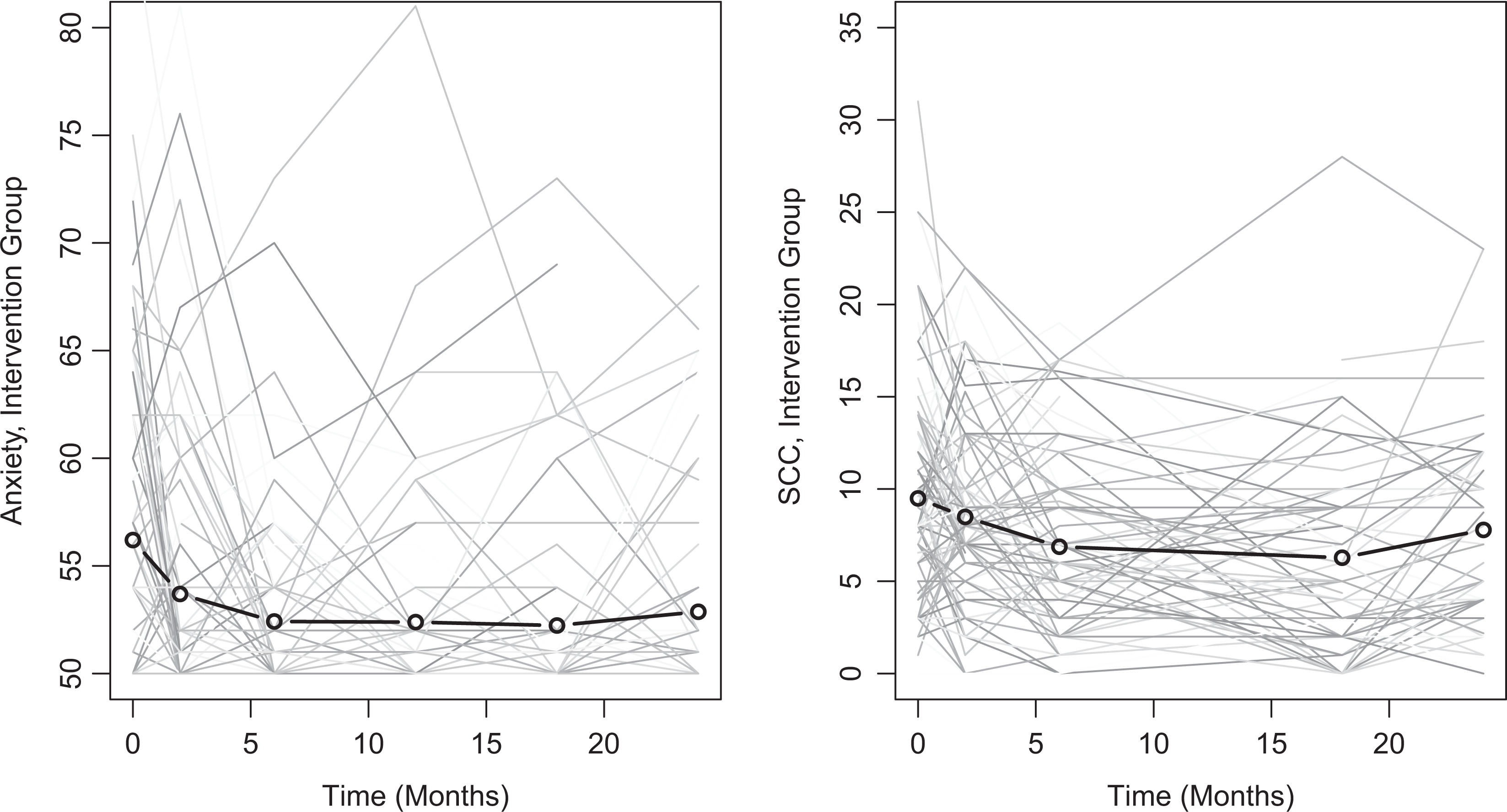
Observed Participants’ Trajectories (Thin Gray Lines) for Anxiety/Depression (Left) and SCC (Right) for the Intervention Group.

An LGCM with only an intercept was fit to the later observations (6–24 months) to examine whether a model that allowed for individuals to have unique means that were constant across time (time invariant) was a reasonable approximation of the data. Models were fit separately for anxiety/depression (four observations, n = 192) and SCC (three observations, n = 187) using full-information maximum likelihood. The random intercept-only LGCMs fit the data relatively well and seem to be a reasonable approximation of the trajectories between 6 and 24 months (CFI_ANX = .978, RMSEA_ANX = .062; CFI_SCC = .962, RMSEA_SCC = .079).

The random intercepts capture the steady-state, time-invariant differences between individuals but do not describe how individuals vary around their individual intercepts. For these data, one could conceptualize the observed indicators at any time to consist of two components: (1) a time-invariant component similar to a random intercept and (2) a time-varying component specified by a SDE model as in equation (1). To separate the time-varying and time-invariant components, an approach in the SEM literature can be used (Hamaker et al., 2015) which, when combined with an SDE, can produce the model depicted in Figure 7. Two variations, Models A and B, are depicted in Figure 7. Both models include effects of level on velocity for both anxiety/depression and SCC; these would allow for a person above or below their intercept to revert back to their intercept.

Figure 7.

The Models Fit to the Intervention Data.

Two models were used to test how the variations in SCC across time are related to anxiety/depression. In Model A, the level of SCC affects the velocity of anxiety/depression. This model posits that one’s level, relative to an individual’s random intercept for SCC, relates to the velocity of anxiety/depression. In Model A, the stochastic perturbations of anxiety/depression and SCC (velocities) are allowed to correlate, as there may be common events that affect both variables. Model B posits a different underlying process where SCC “drives” anxiety/depression, such that changes (velocity) in SCC predict the velocity of anxiety/depression. This model posits that it is not the levels of SCC that relate to change in anxiety/depression, but rather that there are in-tandem changes in SCC driving anxiety/depression.

Model implementation in SEM

Fitting the model in Figure 7 and getting appropriate SDE estimates is the same as any other SEM, with only one exception. To approximate the SDE numerically, the few latent steps depicted between observation occasions in the figure must be expanded to a large number of latent steps (e.g., 100+ latent steps for each 6-month interval). This avoids the need for particularly specialized knowledge in stochastic calculus, although it imposes a programming burden. Typically, convergence must be first achieved with a small number of latent steps, and then the estimated solutions used as start values in models with an iteratively larger number of steps.³ Although time-consuming, iteratively increasing the latent steps allows one to confirm whether the estimated parameters converge to a value as the time between latent steps (dt) approaches zero. A lack of asymptotic convergence is a useful indication that models have been incorrectly specified, are under-identified, or lack sufficient information in the data (empirical under-identification). The online supplement includes plots of the estimated parameters demonstrating the convergence of estimates toward an asymptote parameter with an increasing number of intervening latent variables.

Results and discussion

The Akaike information criterion (AICs) and Bayesian information criterion (BICs) for Model A (level–velocity) and Model B (velocity–velocity) did not show clear support for one model over the other, with the AIC being lower for Model A (AIC_A = 4292.5, AIC_B = 4297.0) and the BIC being lower for Model B (BIC_A = 594.3, BIC_B = 591.7). Although clear support for one model over the other is not supported by these data, examination of the estimates is still informative about different processes. Table 1 presents the estimates for the “Readings” group, the difference between the “Readings” and “Intervention” groups, the standard error of the difference, and the Wald-statistic p value for the difference. Both models estimate similar parameters for the time-invariant parts of the models, the random intercept means (ν_ANX, ν_SCC), variances (ψ_TI,ANX, ψ_TI,SCC), and their covariance (ψ_TI,S-A). In both models, the random effect of anxiety/depression has a statistically lower mean and less variance for the Intervention group compared to the Readings group, as would be typically expected for a successful intervention.

Table 1.

Estimates for Model A (Level–Velocity) and Model B (Velocity–Velocity) With Statistical Tests for Differences in the Parameters Between the “Reading” and “Intervention” Groups.

Parameter	Model A (level–velocity)				Model B (velocity–velocity)
Parameter	Readings	Group Diff	S.E. Diff	p Value	Readings	Group Diff	S.E. Diff	p Value
Random effects (time-invariant)
Mean anxiety/depression (ν_ANX)	55.50	−2.82	0.78	.000	55.49	−2.83	0.79	.000
Mean SCC (ν_SCC)	7.84	−0.89	0.71	.208	7.80	−0.79	0.71	.267
Variance anxiety/depression (ψ_TI,ANX)	33.08	−22.29	7.60	.003	33.32	−22.88	8.15	.005
Variance SCC (ψ_TI,SCC)	20.30	−10.85	6.58	.099	20.94	−8.29	6.56	.206
Covariance anxiety, SCC (ψ_TI,S-A)	14.96	−8.86	5.11	.083	14.93	−5.64	4.83	.243
TV initial covariance
Variance anxiety/depression (ψ_TV,ANX)	15.39	−5.50	5.59	.326	25.30	−12.68	9.17	.166
Variance SCC (ψ_TV,SCC)	−0.09	1.89	3.95	.632	−11.50	9.09	6.26	.146
Covariance anxiety/depression, SCC (ψ_TV,S-A)	12.54	4.59	6.54	.483	13.03	2.40	5.22	.646
Derivative relations
Anxiety/depression level–velocity (β_A)	−1.43	0.60	0.63	.342	−1.55	0.84	0.69	.225
SCC level–velocity (β_S)	−1.69	1.03	0.89	.244	−9.30	8.27	19.45	.671
SCC level to anxiety/depression velocity(β_ModelA)	−0.82	1.17	0.90	.195	—	—	—	—
SCC velocity to anxiety/depression velocity(β_ModelB)	—	—	—	—	0.90	−0.72	0.28	.010
Stochastic perturbations
Variance anxiety/depression (ψ _q _A)	78.02	−53.55	3.22	.021	45.29	−21.75	15.29	.155
Variance SCC (ψ _q _S)	39.59	−10.36	7.34	.550	182.52	−147.28	356.9	.680
Covariance anxiety/depression, SCC (ψ _q _S-A)	36.12	−31.39	5.35	.041	—	—	—	—

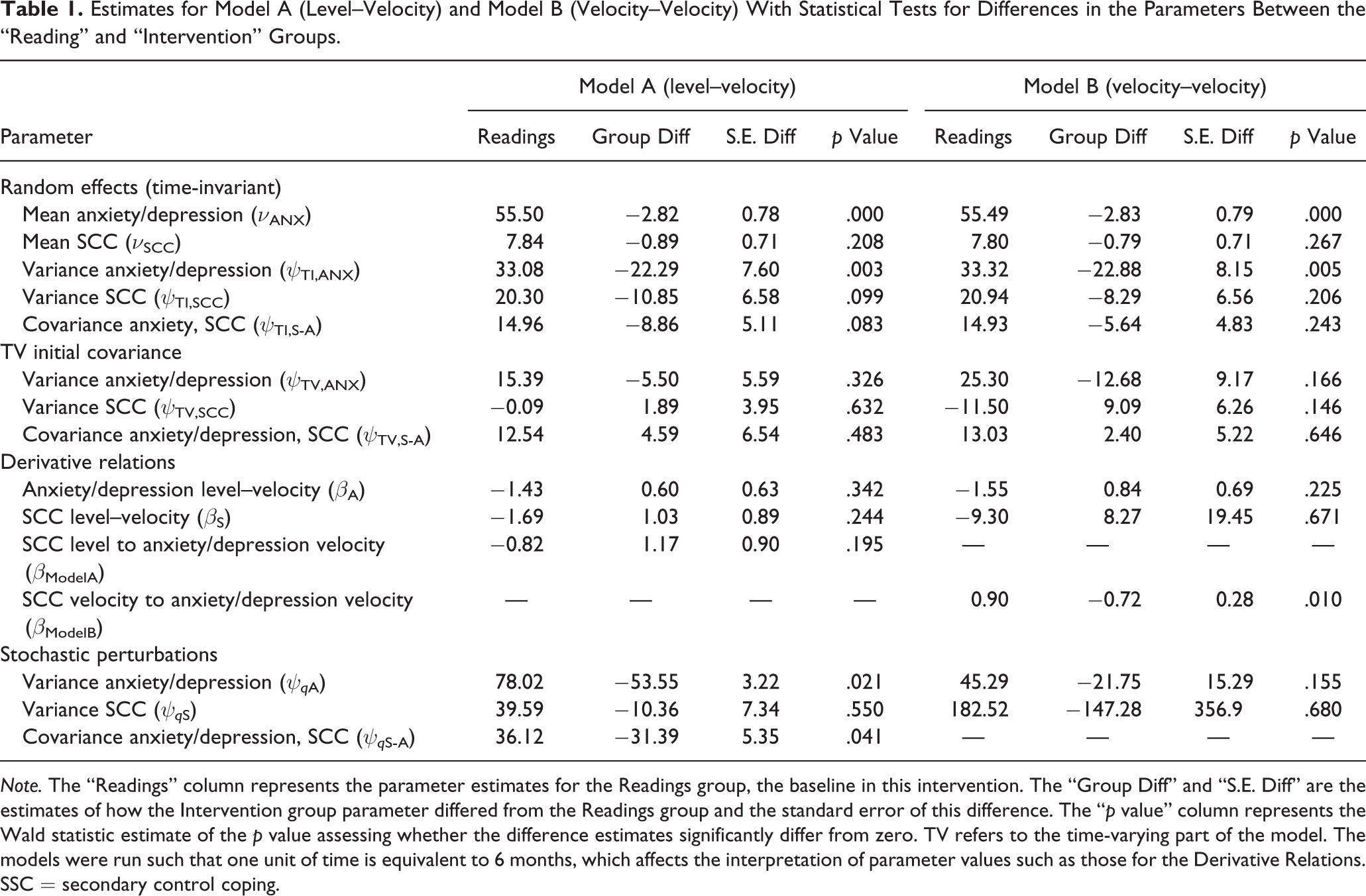
Note. The “Readings” column represents the parameter estimates for the Readings group, the baseline in this intervention. The “Group Diff” and “S.E. Diff” are the estimates of how the Intervention group parameter differed from the Readings group and the standard error of this difference. The “p value” column represents the Wald statistic estimate of the p value assessing whether the difference estimates significantly differ from zero. TV refers to the time-varying part of the model. The models were run such that one unit of time is equivalent to 6 months, which affects the interpretation of parameter values such as those for the Derivative Relations. SSC = secondary control coping.

In the time-varying part of the model, some differences suggest that the intervention may have affected more than the mean and variance of the random effects. In Model A, the variance of the stochastic perturbations for anxiety/depression (ψ _q _A) is significantly lower in the Intervention group (p = .021). This may suggest that participants become better (i.e., more valid) evaluators of their own anxiety/depression as a result of the intervention, such that there is less noise around the trajectories of people who received the intervention. The dynamics within and between variables, however, are not significantly different for the two groups. No evidence is provided that the intervention has changed the regulation of anxiety/depression (anxiety/depression level–velocity, β_A, p = .342) or SCC (SCC level–velocity, β_S, p = .244) across time, nor the effect of the level of SCC on the changes in anxiety/depression (SCC level to anxiety/depression velocity, β_ModelA, p = .195).

Model B offers a different perspective on the data, and another possible way in which the children were affected by the intervention. Model B does not provide evidence for a difference in the stochastic perturbations to anxiety/depression for the two groups (ψ _q _A, p = .155). As with Model A, Model B provides no evidence that the intervention has changed the regulation of anxiety/depression (anxiety/depression level–velocity, β_A, p = .225) or SCC (level–velocity, β_S, p = .671) across time. Model B does, however, suggest that the way in which the velocity (changes) of SCC affects the velocity of anxiety/depression is positive for the Reading group (β_ModelB, β = .90) and significantly closer to zero for the Intervention group (β_ModelB difference = –0.72, p = .010). The positive value for the Reading group suggests that time-varying changes in SCC are positively related to changes in anxiety/depression, but for the Intervention group, the relation might be much closer to zero (i.e., .90–.72 = .18). Alternatively, Model A (where the velocity of SCC and anxiety/depression are correlated) suggests not that one variable affects the other but that events may affect time-varying changes to both anxiety/depression and SCC. This covariance is smaller for the Intervention group in Model A, with the Reading group having a correlation of .65 and the Intervention group a correlation of .18.

Let us emphasize that the purpose of this analysis was not to draw strong conclusions about the intervention. Rather, we present this example to highlight how models with time-varying changes and time-invariant components can be fit to intervention panel data. This example also demonstrates the fitting of an SDE to the time-varying component of the model. In fitting this SDE, we fit models exploring different underlying dynamic processes by changing the level–velocity and velocity–velocity relations. The results suggest a change in mean structure that would be expected for a successful intervention. In addition, however, the time-varying parameters allowed for examination of differences in the regulation of variables (level–velocity within variables), stochastic perturbations around one’s mean, and coupled relations between variables. These parameters may give insight into whether and how the intervention has changed the system dynamics within and between variables.

Conclusions

Many interventions involve collecting repeated observations on the same individuals (e.g., baseline, mid-intervention, two to three post-intervention observations), which offers the opportunity to consider differences in how individuals vary over time. This article presents the possibility of modeling both time-varying and time-invariant effects using SEM and SDEs. The introduction of SDEs allowed for framing nonlinear processes as relations between derivatives. In the substantive example, this procedure allowed for the exploration of two different processes in the time-varying part of the model. Although these processes included regulation within variables, ongoing stochastic perturbations, and different relations between variables, the models were successfully fit to a relatively limited number of repeated observations. Differences in the dynamics of the Reading and Intervention groups became apparent, suggesting that effective interventions may not be limited to changes in means but may also result in changes to how variables affect each other over time.

SDEs offer the opportunity to specify a variety of processes for how individuals change from one time to the next. This offers intervention researchers multiple research opportunities. The variety of differential equations that can be explored, including different relations between derivatives and inclusion of stochastic elements, allows for the exploration of the dynamics within and between variables. These models also offer the opportunity to assess whether an intervention has changed the dynamics of a system, in addition to producing mean differences. Changes to the dynamics of an underlying system may be instrumental to understanding why certain interventions are effective and why the effects of some interventions are more transient. Moreover, certain changes to system dynamics may be important for producing interventions with more sustained effects. Interventions targeting differential self-regulation in anxiety/depression, versus those reducing the variance of perturbations to anxiety/depression, versus those that change the coupling to other variables may be differentially effective. If the key to successful interventions lies in changing dynamics, rather than just producing mean differences, these methods offer a window to understanding how interventions affect the dynamics within and between variables.

Supplemental Material

Supplemental Material, 201912_Additional_Function - Modeling dynamic processes with panel data: An application of continuous time models to prevention research

Supplemental Material, 201912_Additional_Function for Modeling dynamic processes with panel data: An application of continuous time models to prevention research by Pascal R. Deboeck, David A. Cole, Kristopher J. Preacher, Rex Forehand and Bruce E. Compas in International Journal of Behavioral Development

Supplemental Material

Supplemental Material, 201912_Level_to_Velocity_Coupling - Modeling dynamic processes with panel data: An application of continuous time models to prevention research

Supplemental Material, 201912_Level_to_Velocity_Coupling for Modeling dynamic processes with panel data: An application of continuous time models to prevention research by Pascal R. Deboeck, David A. Cole, Kristopher J. Preacher, Rex Forehand and Bruce E. Compas in International Journal of Behavioral Development

Supplemental Material

Supplemental Material, 201912_Primary_Script_(RUN_THIS) - Modeling dynamic processes with panel data: An application of continuous time models to prevention research

Supplemental Material, 201912_Primary_Script_(RUN_THIS) for Modeling dynamic processes with panel data: An application of continuous time models to prevention research by Pascal R. Deboeck, David A. Cole, Kristopher J. Preacher, Rex Forehand and Bruce E. Compas in International Journal of Behavioral Development

Supplemental Material

Supplemental Material, JBD905354_supplemental_figure - Modeling dynamic processes with panel data: An application of continuous time models to prevention research

Supplemental Material, JBD905354_supplemental_figure for Modeling dynamic processes with panel data: An application of continuous time models to prevention research by Pascal R. Deboeck, David A. Cole, Kristopher J. Preacher, Rex Forehand and Bruce E. Compas in International Journal of Behavioral Development

Supplemental Material

Supplemental Material, JBD905354_supplemental_material - Modeling dynamic processes with panel data: An application of continuous time models to prevention research

Supplemental Material, JBD905354_supplemental_material for Modeling dynamic processes with panel data: An application of continuous time models to prevention research by Pascal R. Deboeck, David A. Cole, Kristopher J. Preacher, Rex Forehand and Bruce E. Compas in International Journal of Behavioral Development

Footnotes

Funding

The author(s) declared receipt of the following financial support for the research, authorship, and/or publication of this article: The data for this paper were support by NIH grants R01MH069928 and R01MH069940.

ORCID iD

Pascal R. Deboeck

Supplemental Material

Supplemental material for this article is available online.

Notes

References

Abraham

R. H.

Shaw

C. D.

(2005). Dynamics: The geometry of behavior (4th ed.). Aerial Press.

Achenbach

T. M.

(1991). Integrative guide for the 1991 CBCU4 -18, YSR, and TRF profiles. University of Vermont, Department of Psychiatry.

Beardslee

W. R.

Wright

E. J.

Gladstone

T. R. G.

Forbes

(2007). Long-term effects from a randomized trial of two public health preventive interventions for parental depression. Journal of Family Psychology, 21, 703–713. http://doi.org/10.1037/0893-3200.21.4.703

Bergeman

C. S.

Deboeck

P. R.

(2014). Trait stress resistance and dynamic stress dissipation on health and well-being: The reservoir model. Research in Human Development, 11, 108–125.

Bergstrom

A. R.

(1990). Continuous time econometric modelling. Oxford University Press.

Bettis

A. H.

Forehand

Sterba

S. K.

Preacher

K. J.

Compas

B. E.

(2018). Anxiety and depression in children of depressed parents: Dynamics of change in a preventive intervention. Journal of Clinical Child and Adolescent Psychology, 47, 581–594.

Blanchard

Devaney

R. L.

Hall

G. R.

(2006). Differential equations. Thomson Brooks.

Boker

S. M.

Deboeck

P. R.

Edler

Keel

P. K.

(2009). Generalized local linear approximation of derivatives from time series. In Chow

Ferrer

Hsieh

(Eds.), Statistical methods for modeling human dynamics: An interdisciplinary dialogue (pp. 161–178). Taylor & Francis Group.

Boker

Neale

Rausch

(2004). Latent differential equation modeling with multivariate multi-occasion indicators. In van Montfort

Oud

Satorra

(Eds.), Recent developments on structural equation models (pp. 151–174). Springer.

10.

Bollen

K. A.

(1989). Wiley series in probability and mathematical statistics. Applied probability and statistics section. Structural equations with latent variables. John Wiley & Sons.

11.

Compas

B. E.

Champion

J. E.

Forehand

Cole

D. A.

Reeslund

K. L.

Fear

Hardcastle

Keller

Rakow

Garai

Merchant

M. J.

Roberts

(2010). Coping and parenting: Mediators of 12-month outcomes of a family group cognitive-behavioral preventive intervention with families of depressed parents. Journal of Consulting and Clinical Psychology, 78, 623–634.

12.

Compas

B. E.

Connor

I. K.

Saltzman

Thomsen

A. H.

Wadsworth

(1999). Getting specific about coping: Effortful and involuntary responses to stress in development. In Lewis

Ramsey

(Eds.), Stress and soothing (pp. 229–256). Erlbaum.

13.

Compas

B. E.

Connor

Osowiecki

Welch

(1997). Effortful and involuntary responses to stress: Implications for coping with chronic stress. In Gottlieb

B. H.

(Ed.), Coping with chronic stress (pp. 105–130). Plenum.

14.

Compas

B. E.

Forehand

Keller

Champion

Reeslund

K. L.

McKee

Fear

J. M.

Colletti

C. J. M.

Hardcastle

Merchant

M. J.

Roberts

Potts

Garai

Coffelt

Roland

Sterba

S. K.

Cole

D. A.

(2009). Randomized clinical trial of a family cognitive behavioral preventive intervention for children of depressed parents. Journal of Consulting and Clinical Psychology, 77, 1009–1020.

15.

Compas

B. E.

Forehand

Thigpen

J. C.

Hardcastle

Garai

McKee

Keller

Dunbar

J. P.

Watson

K. H.

Rakow

Bettis

Reising

Cole

Sterba

S. K.

(2015). Efficacy and moderators of a family group cognitive-behavioral preventive intervention for children of parents with depression. Journal of Consulting and Clinical Psychology, 83, 541–553. https://dx-doi-org.web.bisu.edu.cn/10.1037/a0039053

16.

Compas

B. E.

Forehand

Thigpen

J. C.

Keller

Hardcastle

E. J.

Cole

D. A.

Potts

Watson

K. H.

Rakow

Colletti

Reeslund

Fear

Garai

McKee

Merchant

M. J.

Roberts

(2011). Family group cognitive-behavioral preventive intervention for families of depressed parents: 18- and 24-month outcomes. Journal of Consulting and Clinical Psychology, 79, 488–499. https://dx-doi-org.web.bisu.edu.cn/10.1037/a0024254

17.

Compas

B. E.

Keller

Forehand

(2011). Prevention of depression in families of depressed parents. In Strauman

Costanzo

P. R.

Garber

(Eds.), Prevention of depression in adolescent girls (pp. 318–339). Duke University Press.

18.

Deboeck

P. R.

(2019). Empirical Bayes derivative estimates. Multivariate Behavioral Research, 1–23. doi: 10.1080/00273171.2019.1642729

19.

Deboeck

P. R.

Boulton

A. J.

(2016). Integration of stochastic differential equations using structural equation modeling: A method to facilitate model fitting and pedagogy. Structural Equation Modeling, 23, 888–903.

20.

Deboeck

P. R.

Nicholson

J. S.

Bergeman

C. S.

Preacher

K. J.

(2013). From modeling long-term growth to short-term fluctuations: Differential equation modeling is the language of change. In Millsap

R. E.

van der Ark

L. A.

Bolt

D. M.

Woods

C. M.

(Eds.), New developments in quantitative psychology (pp. 427–447). Springer.

21.

Deboeck

P. R.

Nicholson

J. S.

Kouros

Little

T. D.

Garber

(2015). Integrating developmental theory and methodology: Using derivatives to articulate change theories, models, and inferences. Applied Developmental Science, 19, 217–231.

22.

Durrett

(1999). Essentials of stochastic processes (Vol. 1). Springer.

23.

Foa

E. B.

Steketee

Milby

J. B.

(1980). Differential effects of exposure and response prevention in obsessive-compulsive washers. Journal of Consulting and Clinical Psychology, 48, 71–79. http://doi.org/10.1037/0022-006X.48.1.71

24.

Granic

Hollenstein

(2003). Dynamic systems methods for models of developmental psychopathology. Development and Psychopathology, 15, 641–669.

25.

Hamaker

E. L.

Kuiper

R. M.

Grasman

R. P.

(2015). A critique of the cross-lagged panel model. Psychological Methods, 20, 102–116.

26.

Horowitz

J. L.

Garber

Ciesla

J. A.

Young

J. F.

Mufson

(2007). Prevention of depressive symptoms in adolescents: A randomized trial of cognitive-behavioral and interpersonal prevention programs. Journal of Consulting and Clinical Psychology, 75, 693–706. http://doi.org/10.1037/0022-006X.75.5.693

27.

Kanfer

F. H.

Karoly

Newman

(1975). Reduction of children’s fear of the dark by competence-related and situational threat-related verbal cues. Journal of Consulting and Clinical Psychology, 43, 251–258. http://doi.org/10.1037/h0076531

28.

Lindsey

J. K.

(2004). Statistical analysis of stochastic processes in time (Vol. 14). Cambridge University Press.

29.

McArdle

J. J.

Nesselroade

J. R.

(2014). Longitudinal data analysis using structural equation models. American Psychological Association.

30.

Mehta

P. D.

Neale

M. C.

(2005). People are variables too: Multilevel structural equations modeling. Psychological Methods, 10, 259.

31.

Mikosch

(1998). Elementary stochastic calculus, with finance in view (Vol. 6). World Scientific Publishing Company.

32.

Montpetit

M. A.

Bergeman

C. S.

Deboeck

P. R.

Tiberio

S. S.

Boker

S. M.

(2010) Resilience-as-process: Negative affect, stress, and coupled dynamical systems. Psychology and Aging, 25, 631–640.

33.

Nesselroade

J. R.

(1991). Interindividual differences in intraindividual change. In Collins

L. M.

Horn

J. L.

(Eds.), Best methods for the analysis of change: Recent advances, unanswered questions, future directions (pp. 92–105). American Psychological Association.

34.

Newsom

J. T.

(2015). Longitudinal structural equation modeling: A comprehensive introduction. Routledge.

35.

Oravecz

Vandekerckhove

Tuerlinckx

(2009). A hierarchical Ornstein–Uhlenbeck model for continuous repeated measurement data. Psychometrika, 74, 395–418.

36.

Oud

(2006). Comparison of four procedures to estimate the damped linear differential oscillator for panel data. In van Montfort

Oud

Satorra

(Eds.), Longitudinal models in the behavioral and related sciences (pp. 19–39). Routledge.

37.

Oud

J. H.

Jansen

R. A.

(2000). Continuous time state space modeling of panel data by means of SEM. Psychometrika, 65, 199–215.

38.

Shelleby

E. C.

Shaw

D. S.

Dishion

T. J.

Wilson

M. N.

Gardner

(2018). Effects of the family check-up on reducing growth in conduct problems from toddlerhood through school age: An analysis of moderated mediation. Journal of Consulting and Clinical Psychology, 86, 856–867. http://doiorg/10.1037/ccp0000337

39.

Vedeler

Garvey

A. P.

(2009). Dynamic methodology in infancy research. In Valsiner

Molenaar

P. C. M.

Lyra

M. C. D. P.

Chaudhary

(Eds.), Dynamic process methodology in the social and developmental sciences (pp. 431–453). Springer.

40.

Voelkle

M. C.

Oud

J. H.

Davidov

Schmidt

(2012). An SEM approach to continuous time modeling of panel data: Relating authoritarianism and anomia. Psychological Methods, 17, 176.

Supplementary Material

Please find the following supplemental material available below.

For Open Access articles published under a Creative Commons License, all supplemental material carries the same license as the article it is associated with.

For non-Open Access articles published, all supplemental material carries a non-exclusive license, and permission requests for re-use of supplemental material or any part of supplemental material shall be sent directly to the copyright owner as specified in the copyright notice associated with the article.

0.00 MB

0.01 MB

0.00 MB

0.02 MB

0.11 MB