
Abstract
The term ‘configuration’ refers to an arrangement of parts. For example, the elements of a structure constitute a configuration and so do the atoms of a molecule and the components of an electrical network. The most common usage of the term configuration is in reference to geometric compositions that consist of points, lines, surfaces and so on. The term ‘configuration processing’ refers to the skill of dealing with creation and manipulation of configurations. In particular, the term ‘formex configuration processing’ implies configuration processing with the aid of ‘formex algebra’. Formex algebra is evolved to perform processes needed for configuration processing, just as the ordinary algebra is evolved to perform operations needed for creation and manipulation of numerical models. The term ‘formex’ is derived from the word ‘form’ and it is meant to imply a ‘representation of form’. This article has two main objectives. The first objective is to provide a general feeling of how the elements of formex algebra perform configuration processing. This objective is achieved through simple examples, without involvement in too many details. It will be seen that working with parameters is a natural characteristic of formex configuration processing. Thus, a formex solution is, normally, for a class of problems rather than an individual one. This would allow consideration of different variants of a configuration by simply changing the values of the parameters. It will also be seen the ease with which freeforms can be created. The coverage also includes information about ‘Formian’ which is the name of the computer software for formex configuration processing. The second objective of this article is to record the story of the development of formex algebra from the beginnings in the mid-1970s to the middle of the second decade of the 21st century, covering some 40 years of development. Formex configuration processing is an effective and elegant conceptual tool for generation and manipulation of forms. However, there are also other approaches to configuration processing. In particular, there are now a number of highly successful software systems for configuration processing using various tactics. Formex algebra will be a natural complement for these systems.
Background
In May 1963, a research centre called the ‘Space Structures Research Centre’ was established in the Department of Civil Engineering of Battersea College of Advanced Technology in London, UK. The research Centre was founded by the then Head of the Civil Engineering Department, Professor ZS Makowski, with the aim of carrying out fundamental research in all aspects of ‘spatial structures’. Professor Makowski (1922–2005) was a leading expert in the field of spatial structures and devoted his whole career to work in this field. 1
The Battersea College of Advanced Technology later became the ‘University of Surrey’ in 1966 and moved to the town of Guildford near London. Also, the Space Structures Research Centre became a part of the new University and moved to Guildford. The author of this article was a member of the research team at the Centre from the beginning. The aims of the Centre had a wide scope; however, a main research activity of the Centre was the ‘computer aided configuration processing of spatial structures’.
In the 1960s, great advancements were made in digital computer technology, followed by innovative software ideas and high-level computer languages like Algol 60 and FORTRAN. This, in turn, created a suitable environment for major advances in the theory of structures using matrix algebra.
All these were very much welcomed by people working in the field of spatial structures, enabling them to deal with structures having many elements and nodes. It became practical to write computer programs for structural analysis and one of the very first such programs was written in the Space Structures Research Centre in 1964, using a primitive computer language called ‘Sirius Autocode’ for analysis of grids (‘Sirius’ was the name of an early mainframe computer).
However, while enjoying the capabilities of computing facilities for analysis of spatial structures, a new ‘monster’ started to show its face. To elaborate, before the availability of digital computer facilities, all sorts of approximate methods and analogies were being used to analyse structures and these approaches did not involve large amounts of ‘data preparation’. However, when all the elements and nodes of a spatial structure had to be considered in the analysis, the generation of data became a major issue.
Data preparation by hand turned out to be tedious, error prone and time consuming. It was not unusual for the data preparation of a spatial structure with a thousand elements (a relatively small spatial structure) to take 2 or 3 weeks of boring hard work and then the analysis to be performed in a matter of hours by computer.
In the years that followed, the technique that emerged for data generation was to write a computer program for each individual project in a language like Algol 60 or FORTRAN, taking advantage of similarities, repetitions and regularities of the parts of the configuration. By the early 1970s, experience in writing such programs for data preparation showed that some types of procedures recurred frequently and the collection of such recurring procedures resembled the operations of an ‘algebra’.
Early days of formex algebra
In early 1974, the ideas related to an algebraic system for ‘configuration processing’ were written down in a document. 2 The document lays the foundations of a ‘new algebra’. It defines an ‘object’ called a ‘formex’ (plural ‘formices’) consisting of a structured collection of ‘numbers’ for representation of configurations. The document also defines ‘equality’ for formices as well as some ‘operations and functions’ applicable to formices. Indeed, these are the ingredients that constitute an ‘algebra’. Namely, an object together with some ‘relations’, ‘operations’ and ‘functions’. The document contains a number of examples showing how algebraic formulations can be used to represent configurations in a simple and elegant manner.
The document was presented to an invited audience at one of the London offices of the British Steel Corporation in March 1974. Subsequently, a modified version of the document was published as a paper in the International Journal of Computers and Structures, June 1975. 3
Work on formex ideas continued unabatedly and the concepts, terminology and notation kept on improving. The next publication on formex ideas was a conference paper entitled ‘Formex Formulation of Double-layer Grids’. This was presented at a Conference on Spatial Structures, University of Lyon, France, February 1978. 4 A much extended version of this material was written in June 1978 and presented at a Course on ‘Analysis, Design and Construction of Double-layer Grids’ at the University of Surrey in September 1978. 5 A revised version of this material was written in April 1979 and was eventually published in 1981. 6
Early stages of the development of formex algebra continued until the late 1980s. Three major publications that appeared in the period 1984–1985 were as follows: a contribution on the formex formulation of domes by Jaime Sanchez Alvarez, 7 a text book on formex algebra giving a full account of the concepts as they stood in 1984 8 and a book chapter on formex formulation of barrel vaults. 9
Throughout the development of formex ideas, the research students at the Space Structures Research Centre of the University of Surrey made important contributions. Research students working on formex topics in the late 1980s were OFA Al-Labbar, MH Yassaee, Lambros Babilis, Parvindokht Pakandam and Wenxiao Shan.
Algebras have long lives. Also, it takes a long time for an algebra to ‘grow up’. Actually, an algebra never stops growing. However, once one learns to use an algebra, even if it is just the rudiments, then it becomes an effective conceptual tool. And, as the algebra develops further, it becomes more powerful as well as more convenient to use.
Formian: the programming language of formex algebra
Once the basic ideas of formex algebra were established, attempts were made to create a programming language that can be used for execution of formex formulations. Starting in mid-1970s, a programming language called ‘FORMEL’ (standing for ‘formex language’) was defined. 10 However, implementation of FORMEL did not reach a workable stage although its definition later became a useful starting point for the programming language ‘Formian’.
In the meanwhile, in late 1970s, Mahmood Harischian 11 (Heristchian) produced a set of FORTRAN subroutines for formex operations. These subroutines were utilised frequently before the availability of Formian.
Work on the creation of the programming language Formian started in early 1980s. The work involved both the definition of the conceptual constitution of the language (grammar) and the implementation of the definition of the language, that is, production of a software through which the instructions of the language can be executed. The first version of Formian was functional in 1984. 12 The implementation of Formian was led by Peter Disney.
During the years that followed, many ideas for improving Formian were incorporated into the language and a paper containing the definition of Formian was presented at a conference in London in 1989. 13 The paper was later published in the International Journal of Computers and Structures in 1991.
This article, together with its Japanese translation, was also presented at a Symposium on ‘Preprocessing’ in Osaka, Japan, 1990. 14 The Osaka Symposium was organised by Katsuhiko Imai and K Wakiyama who were deeply involved in formex configuration processing. The proceedings of the Osaka Symposium also included a paper (in Japanese) by K Imai regarding the use of formex configuration processing for practical design of spatial structures. Figure 1 shows Peter Disney demonstrating Formian during the Osaka Symposium.
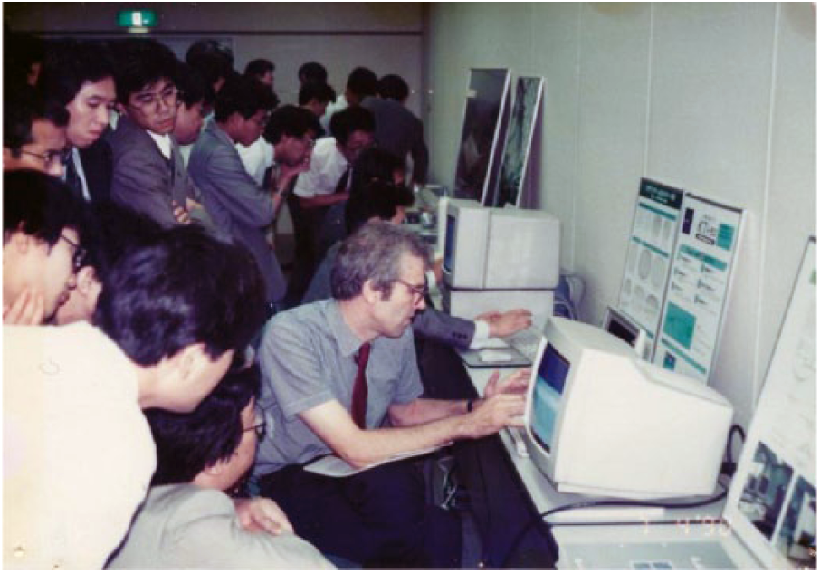
Peter Disney demonstrating Formian during the Symposium on Preprocessing in Osaka, 1990.
In the late 1980s, the Taiyo Kogyo Corporation became involved in the Formian project. Taiyo Kogyo is a well-established Japanese firm of spatial structure constructors and their contribution to the Formian project was of great value. In particular, a highly innovative mathematician, Chiaki Yamamoto, from Taiyo Kogyo, joined the Formian team which benefitted the team substantially. A major step forward at this stage was the writing of a BNF definition of the syntax of Formian which was published in the proceedings of the Symposium on preprocessing in Osaka, 1990 14 (BNF is a language for the precise definition of the syntax of programming languages). Continuation of the improvements in the concepts and implementation resulted in a new version of Formian in 1993. 15
Formian went through another upgrading in the latter part of 1990s, acquiring better screen facilities. The person who was responsible for this upgrading was Nicolas Haywood. The result was a version of Formian that is referred to as Formian-2 and has been in use since then.
How does formex algebra work?
Formex algebra is the central issue in this article and yet no indication of the working of formex algebra has been given so far. The objective of this section is to fill the gap and provide a general notion of what formex algebra is.
Commonly used algebras are ‘number algebra (ordinary algebra)’, ‘matrix algebra’ and ‘Boolean algebra’. Also, ‘formex algebra’ is a new addition to the family of algebras. In what follows, the constitution of an algebra is explained using a simple example from ordinary algebra.
Consider Figure 2 that shows a diamond-shaped quadrilateral with sides of equal length. The diameters of the diamond are denoted by Da and Db and the internal angles are denoted by A and B, where B = 180° − A.

A diamond-shaped quadrilateral.
It is required to derive a formula that gives the relationship between Da and Db.
To solve the problem, one may observe, from the dotted triangle in Figure 2, that
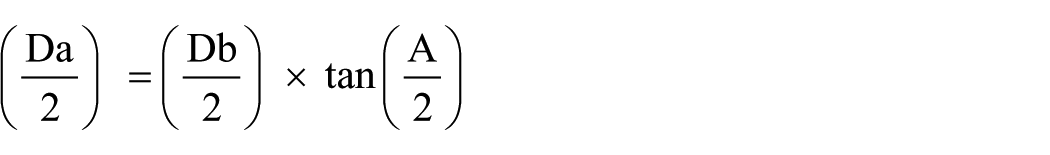
or
This gives the required relationship between the two diameters Da and Db, with ‘A’ being a ‘parameter’. The formula provides a general parametric rule that applies to every diamond shape of any proportions and size. This is the ‘magic of algebra’ that allows ‘general rules’ (parametric rules) to be created so simply. A parametric formulation may also be said to be ‘generic’.
The items employed in the formulation are ‘number’ (denominator of A/2), ‘symbolic representation of number’ (Da, Db and A), ‘relation’ of equality (=), as well as, ‘operation and function’ (multiplication, division and tangent function). Interestingly, in spite of the example being very simple, it involves all the fundamental ingredients of the ordinary algebra.
To elaborate, the constitution of ordinary algebra (number algebra) consists of:
A set of ‘objects’ (the set of all numbers);
A set of ‘relations’ (=, >, <, etc.);
A set of ‘operations and functions’ (+, −, …, sin, cos, etc.).
A constitution of this type is shared by other algebras. Also, the ability of producing ‘parametric formulations’ (generic formulations) is shared by other algebras. For instance, the constitution of ‘formex algebra’ also consists of a set of objects (formices), a set of relations and a set of operations and functions. However, the nature of the ‘objects’, ‘relations’, ‘operations and functions’ of an algebra is such to suit the field of application of that algebra. A simple example is now used to give a feeling of the nature of formex algebra.
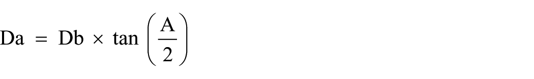
Consider the flat grid that has a diagonal pattern, as shown in Figure 3. Formex algebra may be used to produce a parametric (generic) formulation of this diagonal grid. The grid has a simple form and is suitable as a first example. The grid lies in the X-Y plane and thus the Z-coordinates of all the points of the grid are equal to zero. The overall plan dimensions of the grid are given as L1 and L2 in Figure 3. At a stage of the formulation, the actual geometry of the grid will be represented in terms of X-Y-Z Cartesian coordinates. However, it is convenient to initially formulate the configuration relative to the simple integer coordinates shown in Figure 3 along first and second directions.
A single layer grid with a diagonal pattern.
A configuration can, normally, be formulated in many different ways and the choice of a particular approach depends on the preferences of the user. However, a typical approach in formex configuration processing is to begin by representing a few of the elements explicitly and then using these element as ‘seeds’ for propagation in various ways. This approach is adopted to deal with the formulation of the diagonal grid of Figure 3.
One may start the formulation by representing the ‘cross’ at the left bottom corner of the grid. The elements of this cross are indicated by a, b, c and d. Element ‘a’, in terms of the simple integer coordinates can be represented by [0,0,0; 1,1,0].
This is a ‘formex’ representing the element that connects point ‘0,0,0’ to point ‘1,1,0’. Similarly, elements b, c and d can be represented by formices, as shown at the bottom of Figure 3. Note that in the simple integer coordinate system of Figure 3, the size of divisions along the first direction may be different from that in the second direction.
The whole of the corner cross of the grid may be represented by
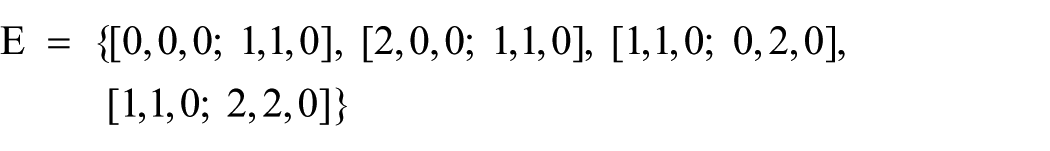
Here, E is a ‘formex variable’ that represents all the four elements of the corner cross. Now, it may be noticed that all the internal elements of the grid can be generated by replicating the corner cross six times in the first direction with the result being replicated four times in the second direction. This double replication may be represented by writing

The term ‘rinid’ is a function name for double translational replication in the first and second directions. The number of replications in the first and second directions is given by 6 and 4 and the ‘pace’ of the replications in the first and second directions is given by 2 and 2. The symbol ‘|’ in the above formula is a ‘separator’ that separates the function from its argument ‘E’. Formex (variable) F is then representing all the internal elements of the grid. To make the formulation parametric, one can write F as

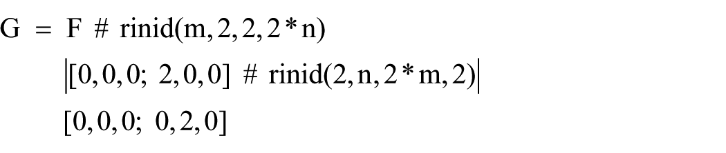
Here, m and n are the numbers of replication in the first and second directions, respectively, as shown in Figure 3. The whole grid including the edge elements may then be represented by

where
The formex [0,0,0; 2,0,0] represents the element indicated by ‘e’ in Figure 3;
The formex [0,0,0; 0,2,0] represents the element indicated by ‘f’ in Figure 3;
The symbol # is the ‘composition operator’ that ‘puts together’ the formices on its left and right.
To complete the formulation, the simple integer coordinates are transformed into actual Cartesian coordinates. This is done by writing

The effect of the ‘bt’ function here is to scale the grid such that the overall dimensions become L1 and L2.
Finally, the complete parametric formulation of the grid will then be


The parameters here are as follows:
Overall length of the grid in the X-direction, L1;
Overall length of the grid in the Y-direction, L2;
Number of crosses in the X-direction, m;
Number of crosses in the Y-direction, n.
For example, using the above formulation, the resulting grids for three choices of parameters are shown in Figure 4.

Three variants of the diagonal grid together with their corresponding parameter values.
A view of the screen of Formian-2 is shown in Figure 5, with the formulation of the diagonal grid of Figure 3 appearing on the left and the plot of the grid appearing on the right of the screen. The parts of the formulation enclosed between compound symbols (*) are ‘comments for information’.
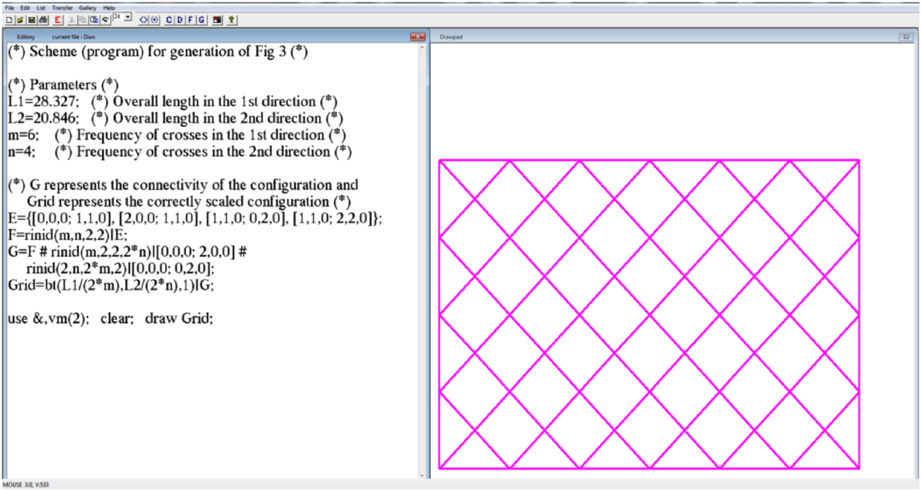
A view of the screen of Formian-2.
In this article, the focus of attention is on configurations of spatial structures. However, formex algebra itself does not have any limitations on the field of application. The algebra can be used in any situation when its conceptual tools may serve to solve problems. In this respect, formex algebra is like the other algebras. Ordinary algebra is employed in so many different fields of application, but it does not belong to any of these fields. Initially, formex algebra has been evolved with spatial structural forms in mind. However, it may also be used in so many other disciplines. It may be used to represent protein molecules or a DNA. It may also be used for the creation of art effects. For instance, Figure 6 shows a painting by the American artist Tony Robbin 16 using Formian. Incidentally, in his article, Tony Robbin also shows examples of four-dimensional (4D) tessellations created using formex algebra. In fact, formex algebra can deal with objects with any number of dimensions.
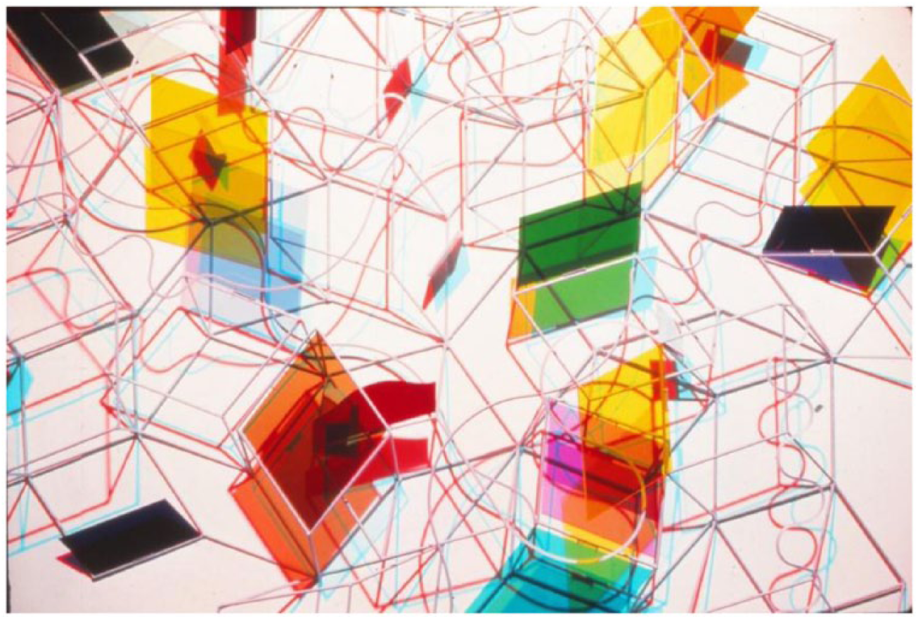
A painting by Tony Robbin using Formian.
Finally, Figure 7 shows samples of patterns created by primary school children using formex formulations.
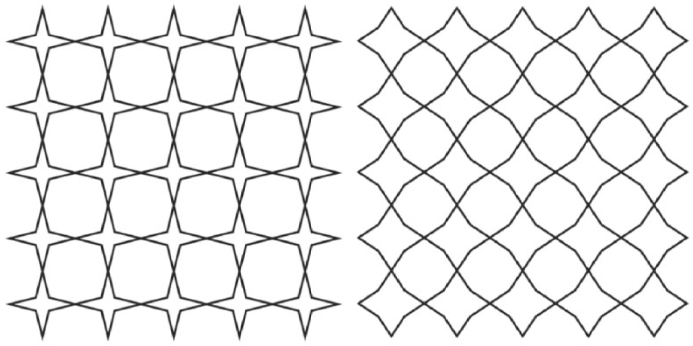
Patterns generated by primary school children using formex algebra.
Actually, experience with children using an elementary subset of the concepts of formex algebra for ‘pattern making’ has been quite successful and there are benefits in introducing the basics of formex algebra at an early age. Figure 8 shows the group of pupils of a primary school, near the University of Surrey in Guildford, UK, visiting the Space Structures Research Centre for their session on ‘formex pattern creation’.
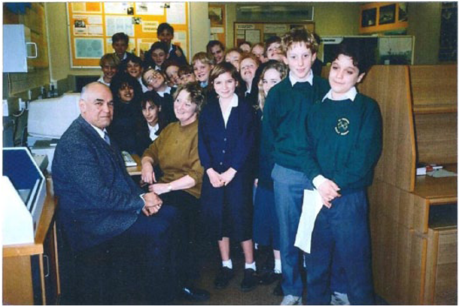
Children visiting the Space Structures Research Centre of the University of Surrey, UK, from a nearby primary school, for their pattern creation session using Formian.
A study regarding the teaching of the elements of formex algebra to school children was carried out by Kirsty McKeon, 17 who was a primary school teacher, in the mid-1980s.
Formex algebra in the 1990s
Last decade of the 20th century turned out to be a highly productive period for formex ideas. With the fundamental basic concepts of formex algebra having reached a good level of maturity and with Formian providing a convenient computing medium for configuration processing, a number of valuable ideas were evolved in the 1990s that enriched formex algebra considerably. Examples are as follows:
Concept of ‘paragenic transformations’, 18 with contributions from Deepali Hadker.
Concept of ‘scallop forms’,19,20 with contributions from Hiroyuki Tomatsuri (Penta-Ocean Construction Co Ltd, Japan) and Masumi Fujimoto (Faculty of Engineering, Osaka City University, Japan).
Concept of ‘pellevation’,21–23 with contributions from Isabell Hofmann.
Development of conceptual tools for dealing with ‘geodesic forms’, with contributions from Dimitra Tzourmakliotou, EE Khalafalla and Oliver Champion.24,25
Concept of ‘novation’, 26 with contributions from FGA Albermani (University of Queensland, Australia). Also, a recent paper provides detailed guidelines for the application of the concept of novation, 27 with contributions from Omidali Samavati.
Development of conceptual tools for form finding of ‘tension structures’, 28 Fevzi Dansik.
Regularisation of spatial structural configurations, 29 with contributions from Koichiro Ishikawa (Fukui university, Japan), John Butterworth (University of Auckland, New Zealand, actually, John Butterworth was a principal member of the research team at the Space Structures Research Centre of the University of Surrey in the 1960s and 1970s). Another researcher involved in this field of work was Yoshihiko Kuroiwa from Tomoe Corporation. 30
Configuration processing of ‘nexorades’ (reciprocal frames),31,32 with contributions from Olivier Baverel.
The concepts of pellevation and novation are particularly useful for parametric formulation of freeforms and their effects will be illustrated here through an example of a flat single layer grid with a ‘honeycomb (hexagonal) pattern’. The plan view of the grid is shown in Figure 9(a), with the overall dimensions being L by L (60 m by 60 m).
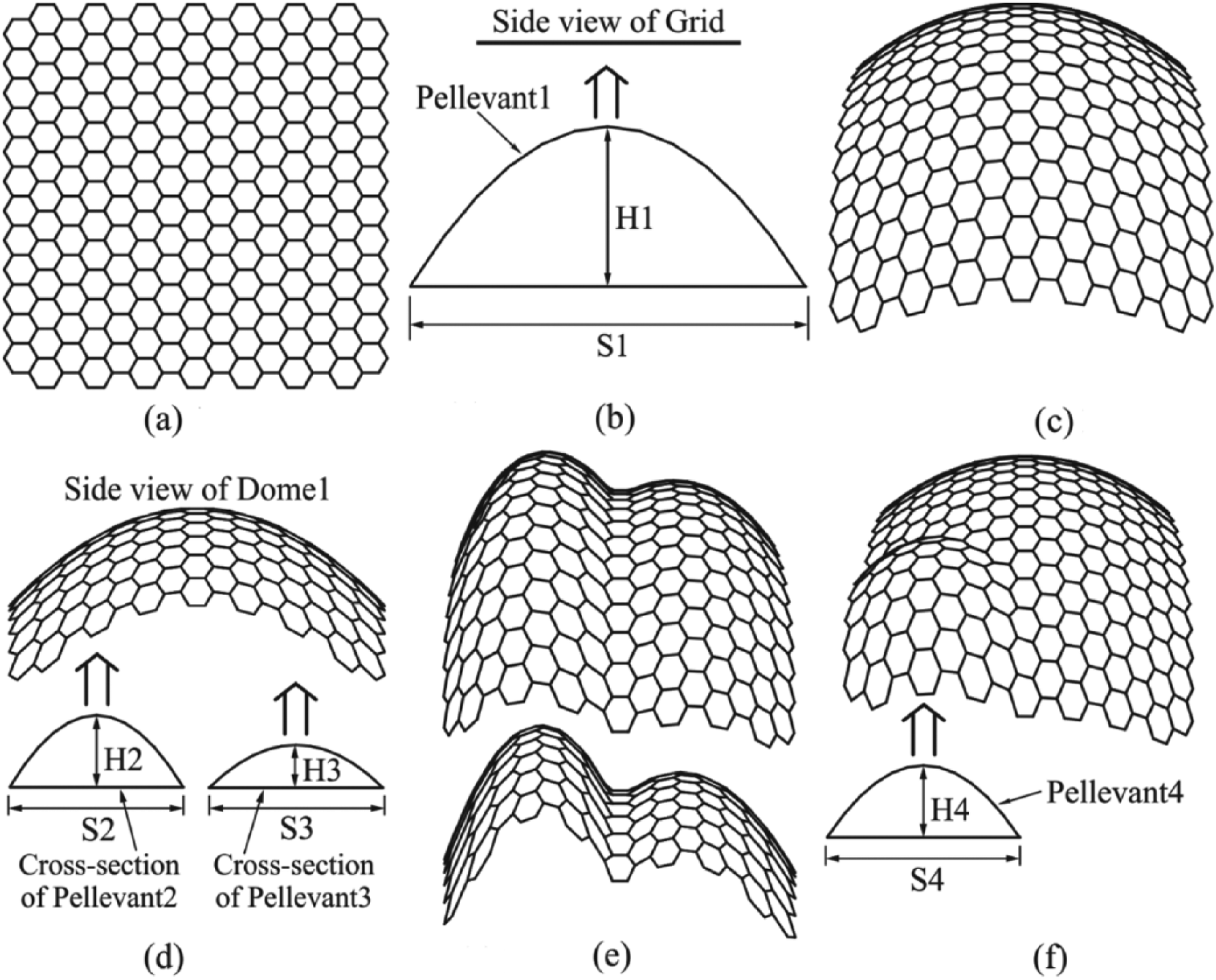
Illustrating the application of the concept of pellevation: (a) Grid, (b) side views of Grid and Pellevant1, (c) Dome1 obtained by pellevating the Grid with Pellevant1, (d) side view of Dome1 with Pellevants 2 and 3, (e) perspective and side views of Dome2 and (f) Dome3 obtained by pellevating of Dome1 with Pellevant4.
The term ‘pellevation’ is a derivative from the Latin word ‘elevare (meaning raise)’. A good way of visualising the effect of pellevation is to think of it as ‘die-stamping’. There are many different shapes of ‘die’ that may be chosen for the process of pellevation and each of these dies is referred to as a ‘pellevant’. Once the type of a pellevant with its size and position are specified, then it will be ‘stamped’ on the given form.
For example, Figure 9(b) shows the side view of the grid of Figure 9(a) (this side view is just a piece of line), together with the side view of a ‘paraboloid of revolution’ which is to be used as a pellevant. This pellevant is referred to as ‘Pellevant1’. The rise of Pellevant1 is chosen to be H1 = 35 m. Also, the span of Pellevant1 is chosen to be S1 = 1.5 L (thus, S1 is slightly larger than the diagonal of Grid). The arrow shape above Pellevant1 in Figure 9(b) indicates the direction of pellevation (stamping). The result of the pellevation of Grid with Pellevant1 is the dome a view of which is shown in Figure 9(c). This dome is referred to as Dome1.
The next stage of the example is illustrated in Figure 9(d), where Dome1 is pellevated again twice with cylindrical pellevants whose cross sections are shown under the side view of Dome1. These pellevants that are called Pellevant2 and Pellevant3 have parabolic cross sections with their span and rise indicated in Figure 9(d).
The pellevation of Dome1 with parameter values S2 = S3 = L/2, H2 = 15 m and H3 = 6 m will give rise to a freeform dome that is referred to as Dome2. A perspective view together with a side view of Dome2 is shown in Figure 9(e). Finally, Dome1 is subjected to another pellevation with a paraboloidal pellevant, called Pellevant4. The outcome of the pellevation with parameter values S4 = 45 m and H4 = 15 m is a freeform dome called Dome3 as shown in Figure 9(f).
The domes generated in the example of Figure 9 relate to the given parameter values. However, many other variants of the domes of Figure 9 may be generated using other possible parameter values.
Another important concept for manipulation of configurations is the concept of ‘novation’. The term ‘novation’ is a derivative from the Latin word ‘novo’ (meaning renew). The effect of novation is to change (renew) the form of a given configuration as guided by specified movements (relocations) of points on or around the configuration.
For example, consider Figure 10(a) that shows a perspective view of the grid of Figure 9(a). The specified movements in this case are as follows:
Corner nodal points numbered 1, 2, 7 and 8 (indicated by dots) are chosen to have zero movement (relocation). That is, the positions of these nodes are to remain fixed.
Nodal points 3 and 6 are chosen to have downward vertical relocations, as indicated by arrows in Figure 10(a).
Nodal points 4 and 5 are chosen to have upward vertical relocations.
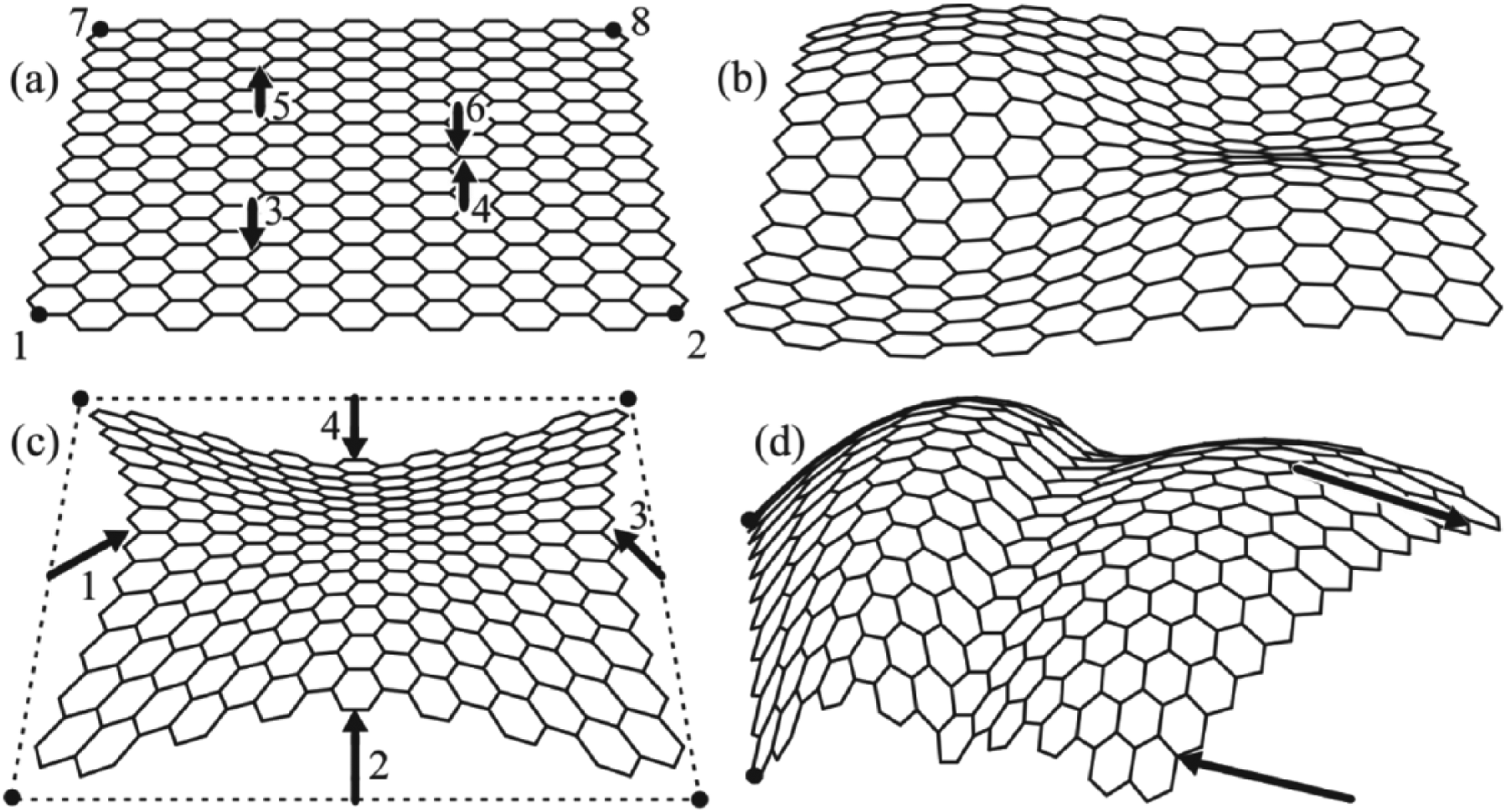
Some examples of the application of novation, as explained in the text.
With these specifications, the ‘novation function’ of Formian will produce the configuration shown in Figure 10(b). Here, all the points that have specified relocations will go through the dictated movements. In addition, the rest of the nodes will follow the trend set by the specified relocations and move in ‘conformity’ (harmony) with the trend. Normally, only a few points have ‘specified relocations’ and the relocations of the other nodes are governed by ‘conformity’.
Figure 10(c) shows another ‘novated’ form of the honeycomb grid of Figure 10(a), where the dotted boundary in Figure 10(c) is the ‘circumscribed square’ of the grid. The specified relocations in this case are as follows. First, the four corners of the boundary (indicated by dots) are to have no movement (their positions are fixed). Also, the midpoints of the edges of the boundary are to have relocations indicated by arrows, where arrows 1 and 3 have upward slope and arrows 2 and 4 have downward slope.
Finally, the pellevated dome of Figure 9(e) is subjected to novation, as shown in Figure 10(d). Here, the specified relocations consist of fixity for two corner nodes at the left, as well as movements for two nodes on the right, as indicated by arrows.
An important point to be noticed here is that the configuration of Figure 10(d) has been subjected to pellevation as well as novation. Actually, in configuration processing, it is a usual practice to create a simple base configuration, to begin with, and then keep on modifying the initial form in various ways to move towards the required shape of the configuration, just as a blacksmith gradually shapes a red hot piece of iron.
Formex algebra in the 21st century, 2000–2015
Good progress has been made regarding formex ideas and Formian during the 21st century so far. Also, major progress was made in another front. Namely, in documenting and publishing the concepts of formex algebra and Formian in order to produce updated material for learning and teaching and as practical guide for the application of formex ideas. To elaborate, three major papers were published in 2000, 2001 and 2002 in the International Journal of Space Structures. The papers are entitled ‘Formex Configuration Processing’ in three parts I, II and III. This collection of papers provides a suitable starting point for learning formex configuration processing. Later, in 2009, these three papers were published as chapters in the book: ‘Structural Morphology and Configuration Processing of Space Structures’. 33
Another two major publications in the field of formex configuration processing appeared in 2005 and 2011. The first one is a book by Janusz Rebielak, 34 entitled ‘Shaping of Space Structures. Examples of Applications of Formian in Design of Tension-strut Systems’. This book contains a rich collection of examples of application of Formian in configuration processing of tension-strut systems. Many of the examples in the book are highly innovative. Also, this book contains an extensive bibliography consisting of some 326 references.
The other publication that appeared in 2011 is a book by Amila Y’Mech, entitled ‘Geodesic Domes: Their geometry and how to use it’. 35 The book provides a practical approach to the generation of geodesic forms using Formian.
Another important project in the period under consideration related to what may be called ‘form tailoring’. This implies creation of a configuration from a combination of (pieces of) different configurations. 36 The researcher involved in this work was Mahdi Moghimi.
Also, reference should be made to the research related to the concept of a ‘plenix’ (plural plenices). A plenix is an object that plays the role of a ‘parametric database’ and has many uses in Formian. The rudiments of the concept of a plenix were evolved in the mid-1970s. These initial ideas were advanced by Mahmood Heristchian (Haristchian) 37 through his PhD research in late 1970s. The next researcher to further improve the theory of plenices in the mid-1980s was Anna Hee. 38 Finally, the plenix ideas were advanced considerably by Masoud Bolourian39,40 in the early years of the 21st century.
Formian-K: the new version of Formian
With the continuous advancement of formex configuration processing concepts and ideas, the need for a major updating of Formian was strongly felt in the recent years. The work on this updating started in 2012 and the updated version was in hand in 2015. The new version is referred to as Formian-K. Among many new and/or improved aspects in Formian-K, the more important additions and/or changes are as follows:
Much improved graphics capabilities.
Addition of extensive programming aids such as looping, subscripting, conditional statements and possibility of creating supplements (user-defined functions).
Extended formex operations (numerex operations).
Improved export facilities, a consequence of which is to increase the ability of Formian to work in combination with other software systems.
New ‘help’ system.
Addition of a ‘gallery’ (of forms) containing over 200 families of spatial structural forms that can be readily used or modified in accordance with the user’s wishes.
Details related to the above items are found in Nooshin et al. 41
A view of the screen of Formian-K is shown in Figure 11. The scheme (program) that is seen on the left is for the generation of the Grid of Figure 9(a), Dome1 of Figure 9(c), Dome2 of Figure 9(e) and the freeform dome of Figure 10(d). The green parts in the scheme are ‘comments for information’. Also, the parameters are listed at the top, and they can be changed as required. The freeform dome of Figure 10(d) is shown in the graphics area on the right.
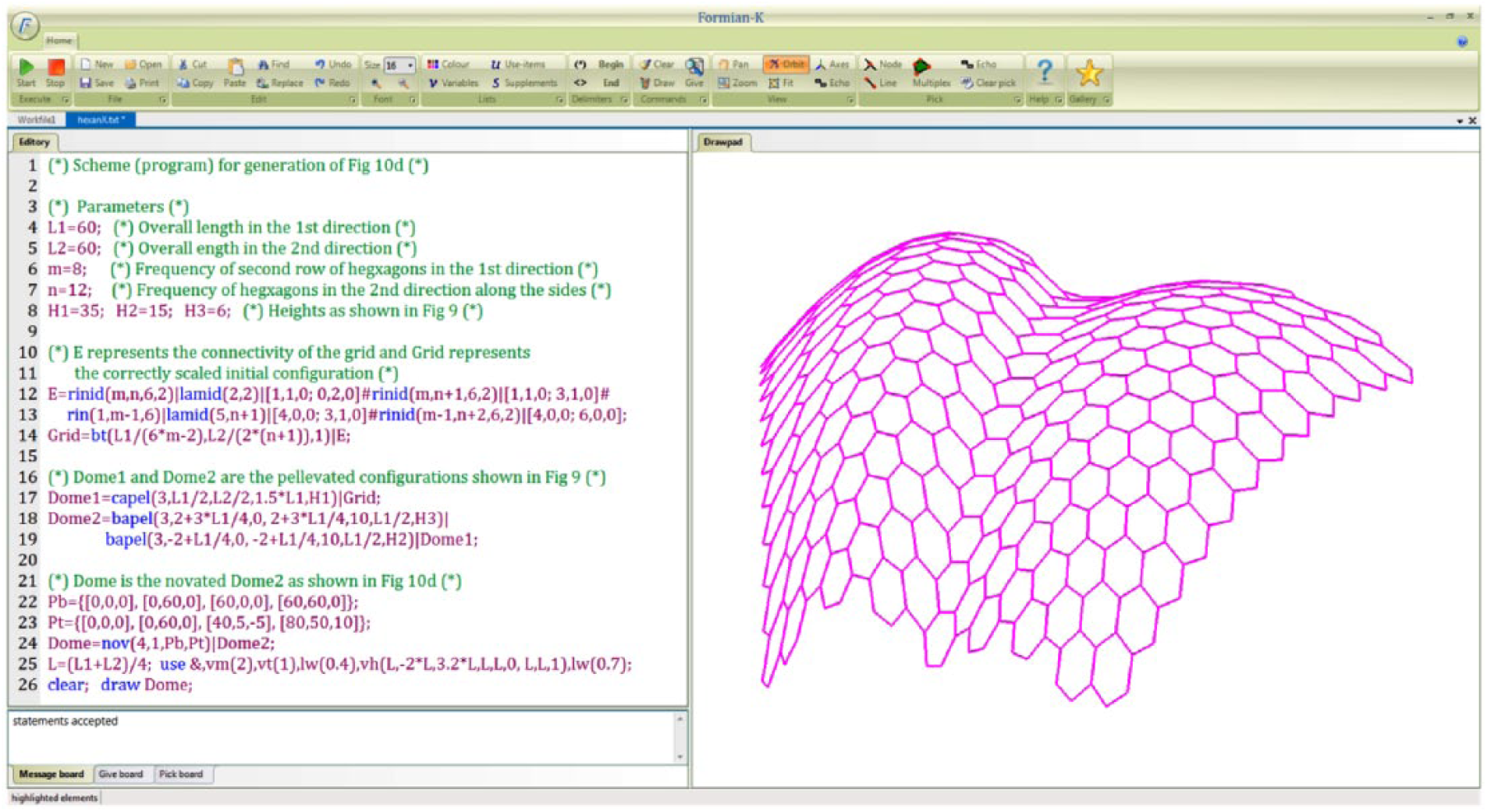
A view of the screen of Formian-K.
The principal people involved in the implementation of Formian-K are Ali Sabzali and Omidali Samavati.
Note: Formexia.com is a website dedicated to the provision of information on formex configuration processing as well as the other aspects of the application of formex ideas and concepts. Also, Formian-2 and Formian-K can be downloaded from this website.
Conclusion
The article has given an overall general feeling for the formex approach in configuration processing. It is demonstrated that the formex concepts provide an effective and convenient way of dealing with configuration processing problems.
Formex algebra turns configuration processing into a serious discipline. A discipline that becomes a well-defined simple conceptual framework for creation and manipulation of forms of all kinds. A discipline that can be taught and learnt at various levels from primary schools to the universities. A discipline that allows configuration processing techniques and procedures to be clearly described and discussed.
Like all conceptual systems, formex configuration processing is a living entity that grows and changes in response to practical needs. Formex configuration processing is a young branch of human knowledge.
Footnotes
Acknowledgements
The early work in formex configuration processing was greatly helped by substantial donations from a group of Iranian engineers. These were A Sarshar, A Jahanshahi, CG Abkarian, GA Mirzareza, MS Yazdani and J Hassanein and their contributions are gratefully acknowledged. Also, during the 1990s, the Taiyo Kogyo Corporation of Japan, NASA (Award No NAGW-4132) and the Tomoe Corporation of Japan were instrumental in supporting research in formex configuration processing. In particular, Yoshito Isono (Taiyo Kogyo Corporation), Kajal Gupta (NASA) and Fujio Matsushita (Tomoe Corporation) were extremely helpful. Their generous contributions are gratefully acknowledged. In the recent years, the Iranian Academic Centre for Education, Culture and Research, Kerman Branch (ACECR) has sponsored the production of Formian-K. In particular, Reza Kamyab (of ACECR) has been very supportive. The help is highly appreciated.
Declaration of conflicting interests
The author(s) declared no potential conflicts of interest with respect to the research, authorship and/or publication of this article.
Funding
The author(s) received no financial support for the research, authorship and/or publication of this article.