Generalizability Theory as a Unifying Framework of Measurement Reliability in Adolescent Research

Abstract

In adolescence research, the treatment of measurement reliability is often fragmented, and it is not always clear how different reliability coefficients are related. We show that generalizability theory (G-theory) is a comprehensive framework of measurement reliability, encompassing all other reliability methods (e.g., Pearson r, coefficient alpha and KR-20, intraclass correlation coefficients). As such, G-theory provides the flexibility and comprehensiveness not offered by conventional reliability methods. Within the G-theory framework, the similarities and differences of different reliability coefficients can be easily understood, and planning for optimal measurement protocols in adolescence research is feasible. Using hypothetical data, we show how different conventional reliability estimates are related to G-theory estimates and how G-theory estimates are obtained in research practice. Adolescence researchers may use G-theory as the general framework for understanding different reliability estimates.

Keywords

reliability generalizability theory intraclass correlation Cronbach’s coefficient alpha interrater reliability Pearson correlation variance components analysis of variance

In adolescence research, as in other social and behavioral sciences, measurement reliability is always an important concern. The meaning and interpretation of our statistical findings hinge on the quality of our measurement data, and reliability is an important aspect of the measurement quality (Wilkinson and the Task Force on Statistical Inference, 1999). As it has been widely discussed in measurement literature, validity is the most fundamental concern in any measurement situation. It is also generally understood that measurement reliability is a necessary, though not sufficient, condition for measurement validity (Brennan, 2006; Crocker & Algina, 1987). The purpose of this article is on measurement reliability, and readers interested in issues related to measurement validity should consult relevant sources in the literature (e.g., Brennan, 2006; Crocker & Algina, 1987; Worthen, White, Fan, & Sudweeks, 1999).

There are different types of reliability estimates, depending on the measurement error sources of interest, such as internal consistency reliability coefficient (Cronbach’s coefficient alpha, KR-20), coefficient of stability (test-retest reliability coefficient), coefficient of equivalence (parallel-form reliability coefficient), and interrater reliability coefficient. In adolescence research and some other areas of psychology, intraclass correlation coefficient is also a widely used reliability estimate for assessing measurement reliability across-raters or across-occasions (e.g., Maisto et al., 2011; Valen, Ryum, Svartberg, Stiles, & McCullough, 2011). Generalizability theory (Brennan, 2010; Cronbach, Gleser, Nanda, & Rajaratnam, 1972), however, has emerged as a comprehensive framework for measurement reliability.

Many adolescence researchers may not be familiar with the generalizability theory (G-theory) and its advantages over conventional forms of reliability estimates (e.g., test-retest reliability, interrater reliability, intraclass correlation, Cronbach’s coefficient α). In this article, we discuss the underlying rationale for different coefficients and present illustrative examples about how the G-theory provides a unified framework for estimating reliability in different situations. We further discuss that the G-theory approach subsumes all other seemingly different reliability coefficients (e.g., intraclass correlations, Cronbach’s coefficient alpha, test-retest reliability) as its special cases. Adolescence researchers may use G-theory as the general framework for understanding different reliability estimates.

Reliability and Its Estimates in Classical True Score Theory

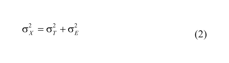
In classical test theory (e.g., Crocker & Algina, 1986; Gulliksen, 1987; Traub, 1994), the observed score (X) from a measurement process (e.g., taking a test, rating provided by an observer) consists of two components: true score (T) and error (E):

X = T + E

Classical true score theory has one basic assumption: the measurement error (E) is random. This basic assumption leads to three resultant assumptions: (a) the mean of errors is zero (μ_E = 0); (b) the correlation between the true score and errors is zero (ρ_T,E = 0); (c) for a population of examinees, errors from two tests (or two forms, two occasions with the same form, two raters, etc.) are not correlated ( $ρ_{E_{1}, E_{2}} = 0$ ). Under these assumptions, the observed score variance ( $σ_{X}^{2}$ ) is the sum of the true score variance ( $σ_{T}^{2}$ ) and the error variance ( $σ_{E}^{2}$ ):

σ_{X}^{2} = σ_{T}^{2} + σ_{E}^{2}

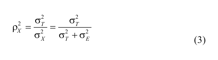
Reliability coefficient ( $ρ_{X}^{2}$ ) is mathematically defined as the ratio of true score variance ( $σ_{T}^{2}$ ) to the observed score variance ( $σ_{X}^{2}$ , often called “total score variance”):

ρ_{X}^{2} = \frac{σ_{T}^{2}}{σ_{X}^{2}} = \frac{σ_{T}^{2}}{σ_{T}^{2} + σ_{E}^{2}}

In other words, a reliability coefficient theoretically represents the proportion of the true score variance ( $σ_{T}^{2}$ ) to the sum of true score variance and error variance ( $σ_{T}^{2} + σ_{E}^{2}$ ).

Equation 3, however, only represents the theoretical measurement reliability. In reality, we only know the observed score variance ( $σ_{X}^{2}$ ). We do not know how much of the observed score variance is true score variance ( $σ_{T}^{2}$ ) and how much is error variance ( $σ_{E}^{2}$ ). Consequently, Equation 3 is not used directly for calculating a reliability coefficient. Instead, we need procedures to estimate the reliability coefficient in a given measurement situation.

Under the assumption of true parallel forms, it can be shown (e.g., Crocker & Algina, 1986) that the correlation coefficient ( $ρ_{X_{1} X_{2}}$ ) between the scores (X₁, X₂) on two parallel forms is theoretically equivalent to the reliability coefficient ( $ρ_{X}^{2}$ ) defined in Equation 3. In other words, although we cannot directly use Equation 3 to obtain the reliability coefficient, we can use the correlation coefficient between two parallel forms as the estimate for the reliability coefficient. There are two assumptions for true parallel forms: (a) each examinee has the same true score on both forms, and (b) the two forms have equal error variances ( $σ_{E 1}^{2} = σ_{E 2}^{2}$ ) (Crocker & Algina, 1986). These two assumptions essentially mean the two tests have (a) equal means (μ₁ = μ₂) and (b) equal variances ( $σ_{X_{1}}^{2} = σ_{X_{2}}^{2}$ ). Traub (1994) provides detailed definition of true parallel tests.

True parallel tests exist in theory only. But when we have measurements that are reasonably parallel, we can estimate reliability coefficient by computing the Pearson correlation coefficient between the two measurements. The two measurements may be obtained in different measurement contexts, such as scores obtained from two test forms (parallel forms), from two occasions (test-retest), or two ratings provided by two raters/observers (interrater), and so forth. The Pearson correlation (as a population parameter) takes the following form:

ρ_{X_{1} X_{2}} = \frac{σ_{X_{1} X_{2}}}{\sqrt{σ_{X_{1}}^{2} σ_{X_{2}}^{2}}}

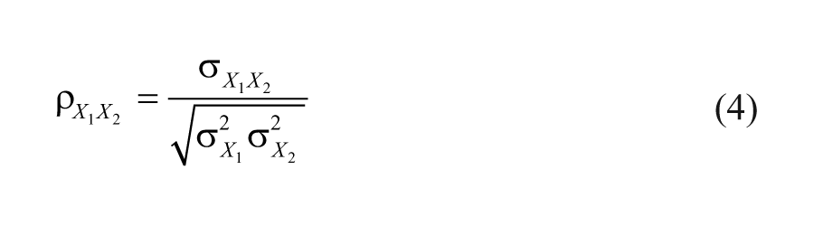
where $σ_{X_{1} X_{2}}$ is the covariance between X₁ and X₂, and $σ_{X_{1}}^{2}$ and $σ_{X_{2}}^{2}$ are the variances for X₁ and X₂, respectively.

Major Types of Reliability Coefficients

Depending on the measurement context, a reliability estimate may take different forms. In classical test theory, there are basically two major forms that a reliability estimate may take: Cronbach’s coefficient alpha and the Pearson correlation coefficient.

Coefficient Alpha

In a situation where a test (i.e., any measurement instrument) involving multiple items is administered to a group of examinees, coefficient alpha (Cronbach, 1951) is the most widely used reliability estimate. Coefficient alpha belongs to the category of reliability estimates for internal consistency of the items, and it takes the following form:

α = \frac{k}{k - 1} (1 - \frac{\sum_{i = 1}^{k} σ_{i}^{2}}{σ_{X}^{2}})

where, k is the number of items, $\sum_{i = 1}^{k} σ_{i}^{2}$ is the sum of item variances ( $σ_{i}^{2}$ ) across all the k items on the test. $σ_{X}^{2}$ is the total score variance. Table 1 illustrates the computation of coefficient alpha for a hypothetical data set of six items (e.g., Likert 6-point scale, 0-5) administered to 10 adolescent respondents. For this small data example in Table 1, α = .86 would generally be considered as representing a high degree of internal consistency among the six response items.

Table 1.

Illustration of Coefficient Alpha Calculation.

	Item
Person	1	2	3	4	5	6	Total score
1	1	0	1	0	4	1	7
2	3	2	3	3	5	3	19
3	4	5	5	4	5	3	26
4	2	2	3	1	3	0	11
5	0	0	1	1	1	0	3
6	3	5	4	4	4	3	23
7	1	1	0	0	4	5	11
8	4	5	4	5	5	1	24
9	2	1	1	0	4	5	13
10	3	3	4	4	5	3	22
Variance	1.61	3.64	2.64	3.56	1.40	3.04	56.69^a
Mean	2.3	2.4	2.6	2.2	4.0	2.4	15.9
$α = \frac{k}{k - 1} (1 - \frac{\sum_{i = 1}^{k} σ_{i}^{2}}{σ_{X}^{2}}) = \frac{6}{6 - 1} (1 - \frac{1.61 + 3.64 + 2.64 + 3.56 + 1.40 + 3.04}{56.69}) = \frac{6}{5} (1 - \frac{15.89}{56.69}) = . 86$

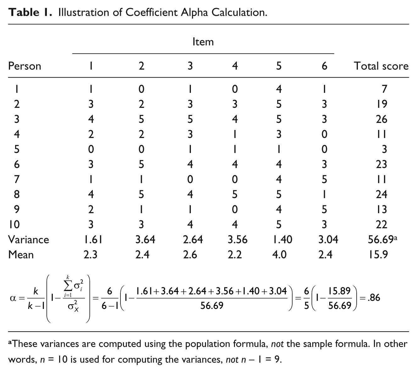
These variances are computed using the population formula, not the sample formula. In other words, n = 10 is used for computing the variances, not n – 1 = 9.

There are other approaches for estimating internal consistency reliability of a test, such as split-half method, KR-20 formula, or Hoyt’s method. Coefficient alpha is theoretically the average of all possible split-half coefficients (Crocker & Algina, 1986). Kuder and Richardson (1937) designed a coefficient (KR-20) for dichotomously scored items, which is a special case of coefficient alpha developed later by Cronbach (1951). Hoyt’s method (Hoyt, 1941) of using an analysis variance model is also equivalent to coefficient alpha algebraically.

Pearson Correlation as Reliability Coefficient

In many situations, the Pearson correlation is used as the reliability coefficient. Computationally, Pearson correlation coefficient can serve as a reliability estimate when there are two sets of scores obtained from one group of examinees (or ratees). Several measurement situations fall under this category: test-retest reliability coefficient, alternate-form reliability coefficient, interrater reliability coefficient. In these situations, the Pearson correlation coefficient between the two sets of scores is computed, and this correlation coefficient is treated as the reliability coefficient. Because reliability coefficient represents the proportion of total (observed) score variance ( $σ_{X}^{2}$ ) contributed to by the true score variance ( $σ_{T}^{2}$ ) (see Equation 3), the Pearson correlation coefficient in this context is a reliability coefficient. As such, conceptually, it already represents the concept of “variance accounted for” (Traub, 1994). For this reason, when used as reliability coefficient, Pearson correlation coefficient should not be squared, and this is contrary to the common practice of squaring correlation coefficient (e.g., coefficient of determination, R², etc.) in many other statistical analyses. Although this point might not be obvious to some readers, the technical illustration for this has been amply provided in psychometric/measurement literature (e.g., Crocker & Algina, 1987; Traub, 1994).

Sources of Measurement Error

As discussed above, different forms of reliability estimates may be obtained, such as Cronbach’s coefficient α (coefficient of internal consistency), interrater reliability coefficient (i.e., coefficient of stability), alternate-form reliability coefficient (i.e., coefficient of equivalence), and interrater reliability coefficient. However, these different forms of reliability estimates are not conceptually equivalent because they capture the measurement error from different sources. For internal consistency (Cronbach’s coefficient α and alternatives), the main source of measurement error is content sampling. For coefficient of stability, the main source of measurement error is time sampling. For coefficient of equivalence, the main source of measurement error is content sampling across forms. For interrater reliability, the main source of measurement error is rater inconsistency (e.g., inconsistent rating criterion for different ratees). Which reliability coefficient to use in a specific measurement situation depends on what measurement error source is the most relevant concern in that situation.

Norm-Referenced Versus Criterion-Referenced Score Interpretation

Norm-Referenced Score Interpretation

Classical true score theory and its reliability procedures were developed for norm-referenced measurement of individual differences. In norm-referenced measurement, the measurement focus is the relative standings of individuals, not the absolute scores. So a typical reliability coefficient (e.g., test-retest reliability coefficient) quantifies the degree of consistency of the relative standings of individuals, but not the consistency of actual scores.

To illustrate the norm-referenced interpretation of a reliability coefficient, Table 2 presents a hypothetical data set in which 10 adolescents (Targets) were rated by two researchers (J₁ and J₂). The interrater reliability coefficient (Pearson correlation) between the ratings provided by J₁ and J₂ is .84, a moderately high interrater reliability coefficient, suggesting that the relative standings of the 10 adolescents are reasonably stable across the two raters.

Table 2.

InterRater Reliability Example.

	Judges
Targets (ratees)	J ₁	J ₂	J₂’
1	52	40	50
2	48	52	62
3	44	48	58
4	40	36	46
5	36	34	44
6	34	44	54
7	30	26	36
8	26	30	40
9	22	18	28
10	18	22	32
Mean	35	35	45
Standard Deviation	11.21	11.21	11.21

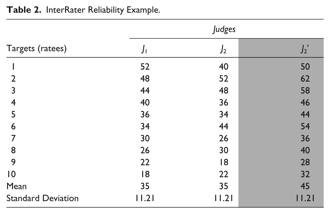
Let’s now assume that the rating from the second judge were really J₂’ (the shaded column). Notice that J₂’ = J₂ + 1. In this situation, it is obvious that the individuals have the same relative positions on J₂ and J₂’, but they have higher scores on J₂’ than on J₂. Classical reliability coefficient only quantifies the consistency of relative standings but not the consistency of actual ratings. As a result, the score difference between J₂ and J₂’ is ignored in classical reliability; the interrater reliability coefficient between J₁ and J₂’ is the same ( $r_{J_{1} J_{2}^{’}} = . 84$ ) as that between J₁ and J₂ ( $r_{J_{1} J_{2}} = . 84$ ). Also, because J₂’ is the linear transformation of J₂ (J₂’ = J₂ + 10), the examinees’ relative standings are exactly the same on J₂ and J₂’. As a result, the Pearson correlation between J₂ and J₂’ is perfect ( $r_{J_{1} J_{2}^{’}} = 1.00$ ), despite the fact that each examinee is 10 points higher on J₂’ than on J₂.

Criterion-Referenced Score Interpretation

In some situations, we are not only concerned about the consistency of relative standings of the individuals (norm-referenced interpretation) but also about the consistency of actual scores (e.g., across testing occasions, across two parallel forms, or across two different raters/observers). In criterion-referenced¹ score interpretation, the measurement interest is not only in the consistency of relative standings but also in the consistency of actual scores. For example, if we are interested in understanding the reliability of the Beck Depression Inventory (BDI) as applied to an adolescent population, it would be grossly insufficient to report only interrater reliability in the form of Pearson correlation coefficient across two raters (norm-referenced reliability). It is crucial that another form of reliability estimate is available that will inform us about the consistency of actual scores across the two raters (criterion-referenced reliability), because the clinical diagnosis of depression depends on the actual score (rating) on BDI. To quantify measurement consistency of both relative standings and actual ratings, we need something different from the Pearson correlation that represents the conventional interrater reliability.

Intraclass Correlation Coefficient (ICC)

Intraclass correlations are rarely discussed in a typical measurement book. For example, a quick look at several measurement books (Crocker & Algina, 1986; Gulliksen, 1987; McDonald, 1999; Traub, 1994) showed that this topic was not covered in any of these books. In adolescence research literature, intraclass correlation coefficient (ICC) has been used widely (e.g., Cicchetti, 1994; Maisto et al., 2011; Brown, West, Loverich, & Biegel, 2011; Valen et al., 2011) although the exact meaning of ICC as used in many research articles in adolescent literature may not always be sufficiently clear. In general, unlike the Pearson correlation coefficient (interrater, test-retest, and parallel form reliability estimates), ICC takes into account both the consistency of relative standings and the consistency of actual scores. ICC relies on the analysis of variance (ANOVA) model to partition score variance into different components. Historically, there has been considerable discussion in the literature on the use of ICCs (e.g., Algina, 1978; Bartko, 1966, 1976, 1978a, 1978b; McGraw & Wong, 1996; Shrout & Fleiss, 1979). Shrout and Fleiss (1979) provided the procedural details for three “Cases” of ICC:

Case 1: ICC(1, 1) or ICC(1, J): Each target is rated by a different set of judges, randomly selected from a larger population of judges;

Case 2: ICC(2, 1) or ICC(2, J): A random sample of J judges is selected from a larger population of judges, and each judge rates all the n targets;

Case 3: ICC(3, 1) or ICC(3, J): Each target is rated by each of the J judges, and these judges are the only judges of interest (i.e., not a sample of judges).

Under each ICC case, the score for each ratee may be represented by a single judge’s rating, or by the average rating of J judges. Statistically, it is well known that the mean score based on J judges is more reliable than the score from a single judge. So reliability may be estimated for the rating of a single judge, ICC(Case #, 1), or for the average scores, each based on J judge, ICC( Case #, J).

Of the three ICC cases discussed in Shrout and Fleiss (1979), Case 2 is the most widely known and used. Case 2 represents a crossed two-way design, with targets crossed with judges, and both factors (“target” and “judge”) are random. For Table 2 data, let’s assume that we have two judges (J₁ and J₂) rating 10 adolescents. Let’s further assume that J₂’ is J₂ transformed (J₂’ = J₂ + 10). If we are concerned about both the consistency of relative standings and the consistency of actual ratings from the two judges, we will use an ICC as the reliability coefficient, rather than interrater reliability in the form of a Pearson correlation coefficient.

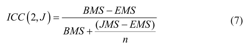
For Case 2 (two-way crossed design), the ANOVA model² contains both “target” (T) and “judge” (J) as the factors. The interaction term between “target” and “judge” (T*J), however, is confounded with error (e) due to insufficient degrees of freedom for separate estimates. Once the score variance is partitioned into different sources through the ANOVA model, the reliability for a single judge’s rating can be computed by the intraclass correlation for Case 2: ICC(2, 1):

I C C (2, 1) = \frac{B M S - E M S}{B M S + (J - 1) E M S + \frac{J (J M S - E M S)}{n}}

where, BMS is the mean square for the targets being rated, EMS is the error (residual) mean square, JMS is the mean square for judges, n is the number of targets, and J is the number of judges. On the other hand, the reliability for the mean scores based on J judges, ICC(2, J), can be obtained from

I C C (2, J) = \frac{B M S - E M S}{B M S + \frac{(J M S - E M S)}{n}}

For Table 2 data, two-way ANOVA provides the needed mean squares for each hypothetical pair of ratings, as shown in Table 3.

Table 3.

Analysis of Variance Results for Data in Table 2.

Source of variance		df	MS
Between J₁ and J₂:
Targets	(BMS)	9	231.11
Judges	(JMS)	1	.00
Residual	(EMS)	9	20.00
Between J₂ and J₂’:
Targets	(BMS)	9	251.11
Judges	(JMS)	1	500.00
Residual	(EMS)	9	.00
Between J₁ and J₂’:
Targets	(BMS)	9	231.11
Judges	(JMS)	1	500.00
Residual	(EMS)	9	20.00

We can compute ICCs for each hypothetical pair of ratings in Table 2:

For J_{1} and J_{2} : I C C (2, 1) = \frac{231.11 - 20.00}{231.11 + (2 - 1) 20.00 + 2 (. 00 - 20.00) / 10} = \frac{211.11}{231.11 + 20.00 - 4} = . 85

I C C (2, J) = \frac{231.11 - 20.00}{231.11 + (. 00 - 20.00) / 10} = \frac{211.11}{231.11 - 2} = . 92 (for J = 2)

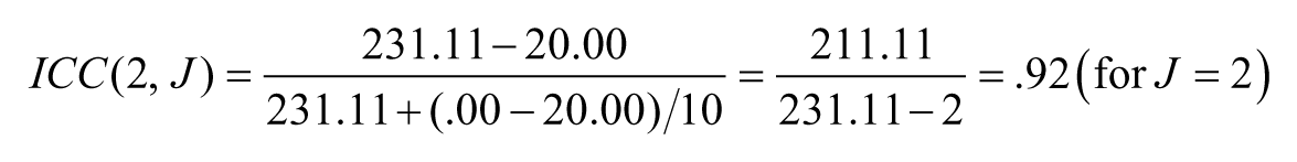
Similarly, we can obtain ICCs for the other hypothetical pairs of ratings:

For J₂ and J₂’: ICC(2, 1) = .72

ICC(2, J) = .83, (for J = 2)

For J₁ and J₂’ : ICC(2, 1) = .61

ICC(2, J) = .76, (for J = 2)

For Table 2 data, the previously computed interrater reliability estimates (Pearson correlations) and the ICCs obtained above are presented in Table 4 for easy comparison. It is shown that, because J₁ and J₂ have the same means, that is, as a group, there is no score change, the ICC(2,1) captures inconsistency in relative standings only; consequently, ICC(2,1) is equivalent to the interrater reliability estimate (Pearson r of .84). Between J₂ and J₂’, however, the relative standings of the ratees are exactly the same across the two ratings; as a result, Pearson correlation coefficient is 1.00, indicating perfect reliability. But because there is rating score change (10 points difference between J₂’ and J₂), the inconsistency of actual rating scores is captured by ICC(2,1) = .72, numerically much lower than interrater reliability of 1.0. Between J₁ and J₂’, there is inconsistency across the two ratings both in the relative standings and in the actual ratings (means of 35 and 45, respectively). As a result, the ICC for J₁ and J₂’ pair of ratings should be the lowest among the three hypothetical pairs of ratings (J₁ vs. J₂, J₂ vs. J₂’, J₁ vs. J₂’ ). ICC(2,1) for J₁ and J₂’ is computed to be .61, considerably lower than the interrater reliability (i.e., Pearson r) of .84.

Table 4.

Interrater Reliability (Pearson r), ICCs and Generalizability Coefficients (for Table 2 Data).

	Hypothetical data pairs
	J₁ vs. J₂	J₂ vs. J₂’	J₁ vs. J₂’
Interrater reliability (Pearson r)	.84	1.00	.84
Intraclass correlations (ICC)
ICC(2,1): Case 2, J = 1	.85^a	.72	.61
ICC(2,2): Case 2, J = 2	.92^b	.83	.76
Generalizability coefficients
For relative decision (ρ²)
J = 1	.84	1.00	.84
J = 2	.91	1.00	.91
For absolute decision (ϕ)
J = 1	.84	.72	.61
J = 2	.91	.83	.76

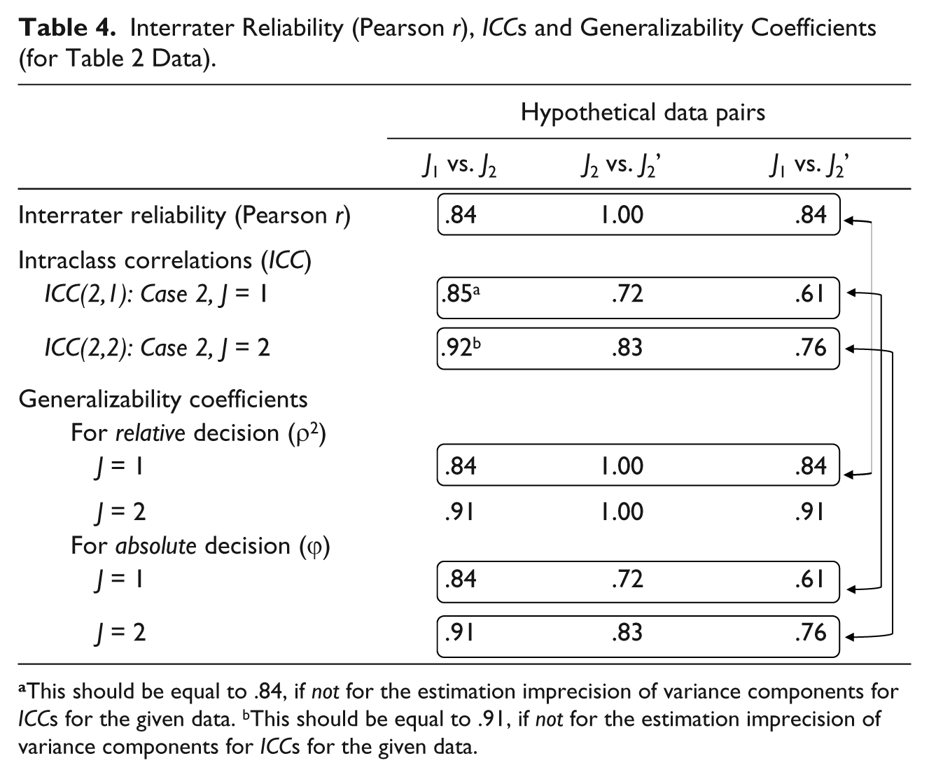
This should be equal to .84, if not for the estimation imprecision of variance components for ICCs for the given data. ^bThis should be equal to .91, if not for the estimation imprecision of variance components for ICCs for the given data.

ICCs for Cases 1 and 3

Because Case 1 and Case 3 ICCs are very rare in adolescence research practice, we will skip these two in this article. Interested readers may refer to Shrout and Fleiss (1979) for details.

Generalizability Theory

In adolescence research, as well as in other behavioral science disciplines, the treatment of measurement reliability is often fragmented. Researchers may be aware of different forms of reliability coefficients, but it could be difficult to understand how different reliability coefficients are related, and what the similarities/differences are among some of these reliability coefficients (e.g., intraclass correlation coefficient vs. interrater reliability coefficient). Generalizability theory (G-theory) provides a comprehensive and unified framework for measurement reliability. G-theory, although widely understood and applied in some disciplines (e.g., educational research and measurement), is not as well known among adolescence researchers. The first comprehensive treatment on G-theory was presented several decades ago (Cronbach et al., 1972). More recent presentations on G-theory (e.g., Brennan, 2010; Cardinet, Johnson, & Pini, 2009; Shavelson & Webb, 1991) have made the G-theory more accessible for research practitioners.

Partitioning Score Variance Into Variance Components

G-theory relies on the analysis of variance (ANOVA) model to partition the total score variance into variance components of different sources. For Table 1 data presented previously, the model appropriate for the data is a crossed two-way ANOVA design, with Person (P) and Item (I) as the two random factors. In this situation, our measurement interest is in the true differences among the persons (P), and this factor is called the “object of measurement.” Factors other than the “object of measurement” are called “facets,” which are potential sources of measurement error. Thus, for Table 1 data, the Item (I) factor is a “facet.” The data collection design in Table 1 is known as one-facet design.

This two-way random-factor ANOVA model means that, theoretically, there are four sources of variation for the scores: Person effect (p), Item effect (i), Person and Item interaction (pi), and finally, the residual (e). But the interaction (pi) and the residual (e) are confounded due to insufficient degrees of freedom. As a result, the total score variance, $σ^{2} (X_{p i})$ , can be partitioned into three variance components: $σ^{2} (X_{p i}) = σ_{p}^{2} + σ_{i}^{2} + σ_{p i, e}^{2}$ .

Variance component estimation relies on the theoretical composition (often called “Expected Mean Square”) of the mean squares for each factor. For the data in Table 1, when an ANOVA is run using both Person (P) and Item (I) as random factors, the results are shown in Table 5. This is a conventional two-way ANOVA summary table, except for the additional column of “Expected Mean Square,” and the variance components derived.

Table 5.

Two-Way ANOVA Summary, Expected Mean Square and Variance Components.

Source	df	Sum of squares	Mean square		Expected mean square
P	9	94.483333	10.498148		$σ_{p i, e}^{2}$ +6 $σ_{p}^{2}$
I	5	22.750000	4.550000		$σ_{p i, e}^{2}$ +10 $σ_{i}^{2}$
Error	45	64.416667	1.431481		$σ_{p i, e}^{2}$
Corrected total	59	181.650000
	Variance component		Estimate	%
	$σ_{p}^{2}$		1.51111	46%
	$σ_{i}^{2}$		.31185	10%
	$σ_{p i, e}^{2}$		1.43148	44%

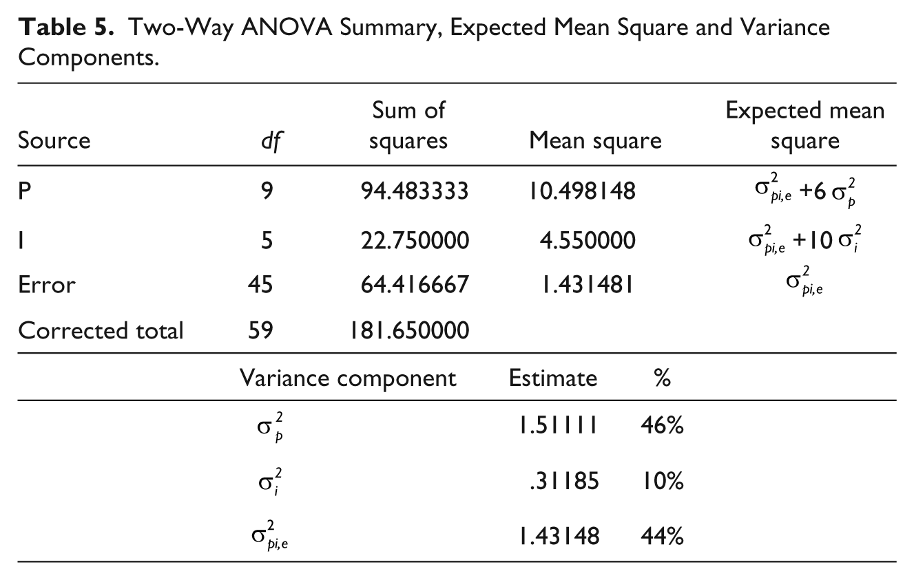
The “Expected Mean Square”³ shows the theoretical composition of each mean square. For example, the residual mean square ( $σ_{p i, e}^{2}$ = 1.431481) theoretically contains both the interaction term p*i and residual e (confounded due to insufficient degrees of freedom). However, the mean square for Factor I (Item) is 4.55, and this quantity theoretically consists of $σ_{p i, e}^{2}$ + 10 $σ_{i}^{2}$ . Because $σ_{p i, e}^{2}$ = 1.431481, we have

4.55 = 1.431481 + 10 σ_{i}^{2},

and we can solve $σ_{i}^{2}$ :

σ_{i}^{2} = (4.55 - 1.431481) / 10 = . 31185

Similarly, the mean square for Factor p is as follows:

10.498148 = 1.431481 + 6 σ_{p}^{2},

and we can solve for $σ_{p}^{2}$ :

σ_{p}^{2} = (10.498148 - 1.431481) / 6 = 1.51111

Because variance components are estimated, the sum of the variance components may be slightly different from the total score variance. Also, there are different approaches for estimating variance components, such as ANOVA approach shown above, or some other method (e.g., maximum likelihood estimation). Statistical software (e.g., SPSS, SAS) provides users with these estimation options.

Similar analyses for variance components for Table 2 data (ratings of 10 adolescent Targets by two Judges)⁴ were conducted, and Table 6 presents the results for the three pairs of ratings in Table 2. In Table 6, $σ_{T J, e}^{2}$ is the variance component of residual plus the interaction term (confounded due to insufficient degrees of freedom). $σ_{J}^{2}$ is the variance component due to Judges, and $σ_{T}^{2}$ is the variance component of Targets.

Table 6.

Estimated Variance Components for Table 2 Ratings.

Between J₁ & J₂:
Variance component	Estimate	%
$σ_{T}^{2}$	105.5556	84%
$σ_{J}^{2}$	–2.0000	0% (⇒ .0000)^a
$σ_{T J, e}^{2}$	20.0000	16%
Between J₂ & J₂’:
Variance component	Estimate	%
$σ_{T}^{2}$	125.5556	72%
$σ_{J}^{2}$	50.0000	28%
$σ_{T J, e}^{2}$	.0000	0%
Between J₁ & J₂’:
Variance component	Estimate	%
$σ_{T}^{2}$	105.5556	61%
$σ_{J}^{2}$	48.0000	28%
$σ_{T J, e}^{2}$	20.0000	12%

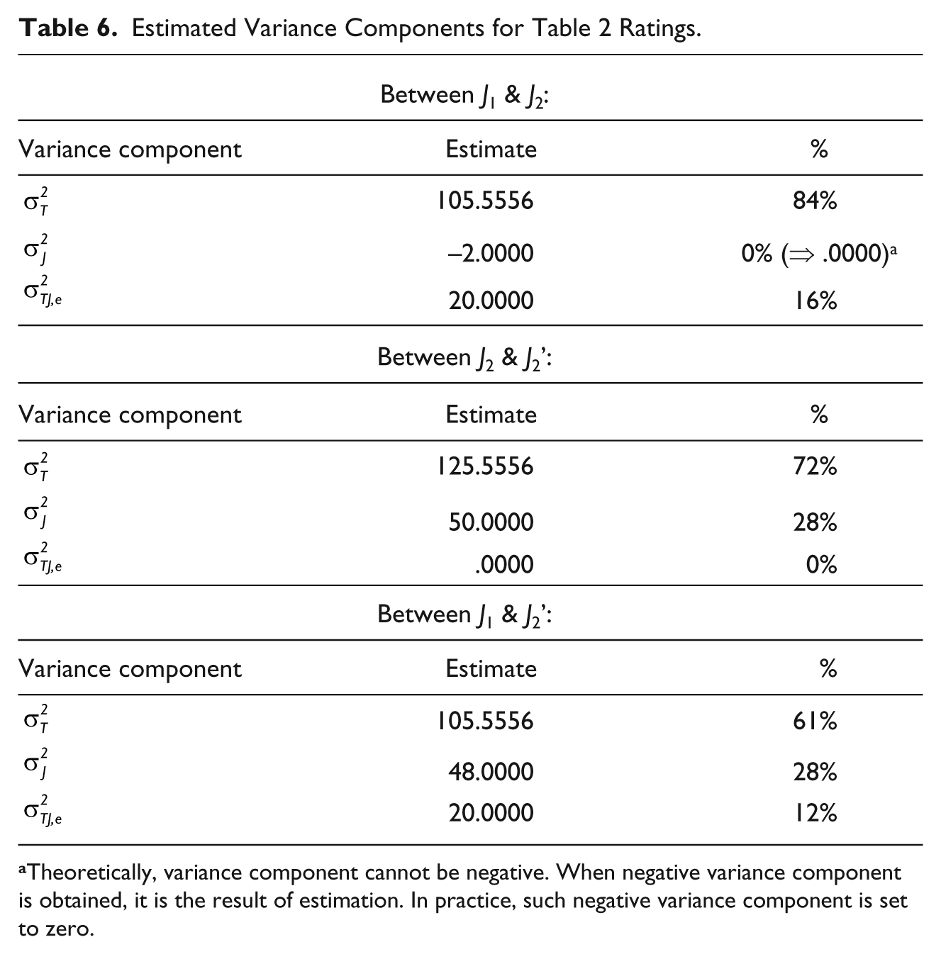
Theoretically, variance component cannot be negative. When negative variance component is obtained, it is the result of estimation. In practice, such negative variance component is set to zero.

Once the variance components are obtained, they will serve as the basis for calculating generalizability coefficients (i.e., reliability coefficients). How the variance components of different sources will be used in a specific study depends on the study design and on the purpose of the measurement interpretation, as discussed in the following sections.

G-Theory Perspectives on Reliability

Relative decision

Classical test theory focuses on norm-referenced score interpretation, that is, using measurement scores to differentiate examinees. As a result, measurement reliability is concerned about the consistency of relative standings of the individuals but not about the consistency of the actual scores. As long as the relative standings of the examinees are consistent, the actual scores do not matter. Within the G-theory framework, this type of interpretation is called “relative decision.”

Absolute decision

Criterion-referenced score interpretation is concerned about both the consistency of the relative standings of the individuals and the consistency of actual scores (i.e., possible score change). This criterion-reference perspective is called “absolute decision” in G-theory.

In a measurement situation, the type of score interpretation (norm- vs. criterion-referenced) determines whether the “relative decision” or “absolute decision” is appropriate. As a result, there are two types of generalizability coefficients: one for “relative decision” reliability and the other for “absolute decision” reliability. The “relative decision” generalizability coefficient is often called ρ², and the “absolute decision” generalizability coefficient is often called φ (Brennan, 2010; Shavelson & Webb, 1991). The difference between the two types of coefficients is on the sources of variation that would be considered as measurement error.

Meaning of Variance Components

Reliability coefficient can be calculated once we know the true score variance ( $σ_{T}^{2}$ ) and the error variance ( $σ_{E}^{2}$ ) (see Equation 3). To understand the estimates for these terms, we need to understand the meaning of the different variance components partitioned previously.

For Table 1 data, that is, six items (I) administered to 10 persons (P), we obtained three variance components shown in Table 5 ( $σ_{p}^{2}$ , $σ_{i}^{2}$ , $σ_{p i, e}^{2}$ ). $σ_{p}^{2}$ represents the variation due to the performance difference among the persons (P), and this is our measurement interest, i.e., this source of variation represents our “object of measurement.” As a result, $σ_{p}^{2}$ is the estimate for the true score variance ( $σ_{T}^{2}$ ) in Equation 3. $σ_{i}^{2}$ represents the variation in the scores due to item “effect.” This is shown by the different means of Item 1 through Item 6 in Table 1 (2.3, 2.4, 2.6, 2.2, 4, and 2.4, respectively). This indicates that examinees’ scores may be higher or lower depending on which items they encounter. This, however, is a consistent effect for all the respondents that will affect respondents’ actual scores but will not affect their relative standings. $σ_{p i, e}^{2}$ represents two confounded sources of variation: random variation (e: random measurement error) and the interaction effect of person by item (p*i). The p*i interaction effect indicates that the item effect is not consistent for all the respondents; as a result, it will affect both the respondents’ relative standings and their absolute scores. Similarly, the random measurement error may also affect both the relative positions and the absolute scores of the respondents. In other words, $σ_{p i, e}^{2}$ brings the two effects (random effect and interaction effect) together.

For Table 2 data of 10 targets (T) rated by two judges (J), the meanings of the variance components (contained in Table 6) are similar. $σ_{T}^{2}$ represents the variation among the Targets (“object of measurement”), and it is the estimate of the true score variance. $σ_{J}^{2}$ represents the effect of judges (e.g., one judge is more stringent than the other in his or her ratings). In Table 2 data, between J₁ and J₂, there is no judge effect, because the average ratings from the two judges are the same (35). On the other hand, between J₂ and J₂’ there is a judge effect because the average rating for J₂’ is 45 vs. 35 for J₂. This effect only affects the actual ratings assigned to the targets, not their relative standings. $σ_{T J, e}^{2}$ contains both the interaction between targets and judges (T*J), and the random measurement error. The interaction effect indicates that the leniency/stringency of a judge is not consistent across the targets, thus both the relative standings and the actual ratings of the targets may be affected by this interaction. Random measurement error also affects both the relative standings and the actual scores.

Measurement Error and Generalizability Coefficients

Generalizability coefficient for Table 1 data

Once we understand the substantive meanings of the variance components, it is relatively easy to construct appropriate generalizability coefficients for “relative” or “absolute” decisions by applying Equation 3. For Table 1 data, we indicated that the item effect ( $σ_{i}^{2}$ ) does not affect the relative standings of the respondents, but only their absolute scores. The person × item (p*i) interaction effect plus random measurement error ( $σ_{p i, e}^{2}$ ) affects both the relative standings and the absolute scores. So for generalizability coefficient of a “relative” decision, the appropriate error term is $σ_{p i, e}^{2}$ . But for generalizability coefficient of “absolute” decision, the appropriate error term is $σ_{i}^{2}$ + $σ_{p i, e}^{2}$ .

We previously computed coefficient alpha for Table 1 data (α = .86). Coefficient α is a reliability estimate for norm-referenced score interpretation; as such, it reflects the consistency of examinees’ relative standings but not the consistency of examinees’ absolute scores. The generalizability coefficient for a “relative” decision is equivalent to coefficient α. If we use Equation 3, and substitute appropriate variance components, we have the following “relative decision” generalizability coefficients for k = 1 (one-item test) and k = 6 (six-item test):

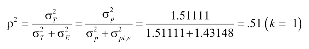
ρ^{2} = \frac{σ_{T}^{2}}{σ_{T}^{2} + σ_{E}^{2}} = \frac{σ_{p}^{2}}{σ_{p}^{2} + σ_{p i, e}^{2}} = \frac{1.51111}{1.51111 + 1.43148} = . 51 (k = 1)

ρ^{2} = \frac{σ_{T}^{2}}{σ_{T}^{2} + σ_{E}^{2}} = \frac{σ_{p}^{2}}{σ_{p}^{2} + σ_{p i, e}^{2} / k} = \frac{1.51111}{1.51111 + 1.43148 / 6} = . 86 (k = 6)

It is noted that for k = 6, the generalizability coefficient is the same as the coefficient α (.86). This is not a coincidence, and it demonstrates that generalizability theory subsumes coefficient alpha. The reason that generalizability (reliability) coefficient for k = 6 is higher (.86) than for k = 1 (.51) is that other things being equal, more items reduce measurement error and produce more reliable measurement.

Generalizability coefficients for Table 2 data

The hypothetical data in Table 2 represent several scenarios. Between J₁ and J₂, the average ratings from two judges are the same (35), thus there is no Judge (J) effect. But there is inconsistency in the relative standings of the ratees (Targets, T) across the two ratings. Between J₂ and J₂’, the ratees are perfectly consistent in their relative standings across the two ratings, but their absolute ratings are not consistent, as shown by the 10 points change from J₂ to J₂’. Between J₁ and J₂’, however, there is inconsistency both in the relative standings and in the absolute ratings.

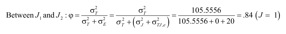
If we are only concerned about the consistency of the relative standings of the ratees across the two ratings (J₁ vs. J₂, J₂ vs. J₂’, or J₁ vs. J₂’), the appropriate error term for generalizability coefficients of “relative decision” (ρ²) should be $σ_{T J, e}^{2}$ , and the coefficients (ρ²) are obtained as shown below:

Between J_{1} and J_{2} : ρ^{2} = \frac{σ_{T}^{2}}{σ_{T}^{2} + σ_{E}^{2}} = \frac{σ_{T}^{2}}{σ_{T}^{2} + σ_{T J, e}^{2}} = \frac{105.5556}{105.5556 + 20} = . 84 (J = 1)

ρ^{2} = \frac{σ_{T}^{2}}{σ_{T}^{2} + σ_{E}^{2}} = \frac{σ_{T}^{2}}{σ_{T}^{2} + σ_{T J, e}^{2} / n_{J}} = \frac{105.5556}{105.5556 + 20 / 2} = . 91 (J = 2)

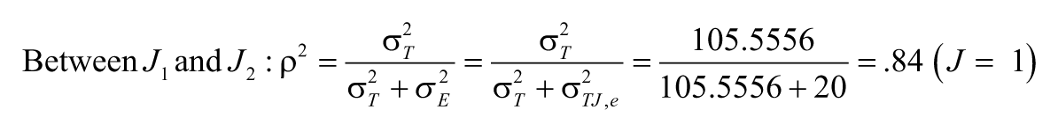
Similarly, we can obtain ρ² for the other two hypothetical pairs of ratings:

Between J₂ and J₂’: ρ² = 1.00 (J = 1); ρ² = 1.00 (J = 2)

Between J₁ and J₂’: ρ² = .84 (J = 1); ρ² = .91 (J = 2)

These relative G-coefficients are presented in Table 4 for easy comparisons with the interrater reliability coefficients (Pearson r) and ICCs. We note that the relative generalizability coefficients for J = 1 (i.e., reliability for only one judge’s rating) and the interrater reliability coefficients (i.e., Pearson correlation coefficients) are equal. As we discussed before, the Pearson correlation coefficient (r) quantifies the consistency of relative standings; as a result, it is conceptually equivalent to the generalizability coefficient for a relative decision (ρ²). Mathematically, however, Pearson r and ρ² are only equivalent when the two ratings have the same standard deviations, as is the case in Table 2 data (SD = 11.21). When the two standard deviations are not equal, Pearson r will be higher than ρ², but the demonstration for this is beyond the scope of this article.

The intraclass correlations in Table 4 are about the consistency of both relative standings and actual ratings, thus they are conceptually equivalent to the generalizability coefficient for absolute decision (φ), and the appropriate error term should be $σ_{J}^{2}$ + $σ_{T J, e}^{2}$ . Using variance components previously obtained (Table 6), these generalizability coefficients (φ) are computed, and we note that these absolute decision coefficients (φ) are equivalent to the ICC(2, 1) and ICC(2, J) presented in Table 4:

Between J_{1} and J_{2} : φ = \frac{σ_{T}^{2}}{σ_{T}^{2} + σ_{E}^{2}} = \frac{σ_{T}^{2}}{σ_{T}^{2} + (σ_{J}^{2} + σ_{T J, e}^{2})} = \frac{105.5556}{105.5556 + 0 + 20} = . 84 (J = 1)

φ = \frac{σ_{T}^{2}}{σ_{T}^{2} + σ_{E}^{2}} = \frac{σ_{T}^{2}}{σ_{T}^{2} + (σ_{J}^{2} + σ_{T J, e}^{2}) / n_{J}} = \frac{105.5556}{105.5556 + (0 + 20) / 2} = . 91 (J = 2)

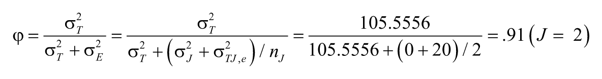
Similarly, we can obtain φ for the other two hypothetical pairs of ratings:

Between J₂ and J₂’: φ = .72 (J = 1); φ = .83 (J = 2)

Between J₁ and J₂’: φ = .61 (J = 1); φ = .76 (J = 2)

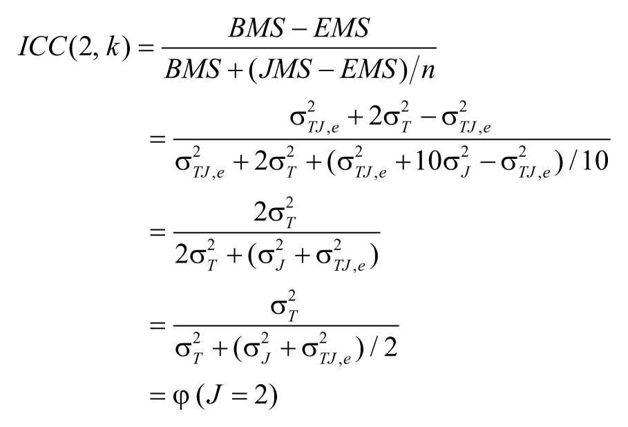
Equivalence of Generalizability Coefficients and Intraclass Correlations

It was shown above that the absolute decision G-coefficients φ are equivalent to intraclass correlation coefficients (Case 2 ICC). This is because the two types of coefficients are mathematically equivalent. For example, it is easy to show that ICC(2, J) is mathematically equivalent to absolute-decision G-coefficient φ when the mean of J = 2 judges’ ratings is used:

\begin{array}{l} I C C (2, k) = \frac{B M S - E M S}{B M S + (J M S - E M S) / n} \\ = \frac{σ_{T J, e}^{2} + 2 σ_{T}^{2} - σ_{T J, e}^{2}}{σ_{T J, e}^{2} + 2 σ_{T}^{2} + (σ_{T J, e}^{2} + 10 σ_{J}^{2} - σ_{T J, e}^{2}) / 10} \\ = \frac{2 σ_{T}^{2}}{2 σ_{T}^{2} + (σ_{J}^{2} + σ_{T J, e}^{2})} \\ = \frac{σ_{T}^{2}}{σ_{T}^{2} + (σ_{J}^{2} + σ_{T J, e}^{2}) / 2} \\ = φ (J = 2) \end{array}

For research methodologists, the equivalence between ICC and generalizability coefficient φ has long been well known. As Shrout and Fleish (1979) discussed, ICC was a special case of the one-facet generalizability study. Although not discussed or presented in this article, it could be shown that other cases of ICC (Case 1 and Case 3) are also special cases of the generalizability coefficients involving nested (Case 1) and fixed (Case 3) factors.

Advantages of Generalizability Theory

The presentation and discussion above have shown that G-theory and its coefficients subsume other types of reliability coefficients, and it provides a unified framework for measurement reliability. It is shown that (a) the G-coefficient (relative decision) is equivalent to coefficient alpha (including KR-20 for dichotomously scored items); (b) G-coefficient (relative decision) is conceptually the same as the reliability coefficients based on Pearson r (i.e., interrater, test-retest, and parallel form reliability coefficients), and it is mathematically equivalent to Pearson r when the two scores to be correlated in Pearson r have equal variances; (c) G-coefficient (absolute decision) is both conceptually and mathematically equivalent to ICCs. However, application of G-theory compels a researcher to make a clear distinction between norm-referenced (relative decision) and criterion-referenced (absolute decision) score interpretations, thus avoiding potential confusion about the appropriateness of some seemingly similar coefficients (e.g., interrater reliability vs. ICC). In addition, G-theory also offers some other important advantages as discussed in the following sections.

Multiple Sources of Measurement Error

Up to now, we have limited our discussion to measurement situations that involve only one “facet” (one measurement error source, other than random measurement error). For example, “item” is the only facet for Table 1 data, and “judge” is the only facet for Table 2 data. Some measurement situations may involve more than one facet, that is, more than one sources of measurement error. Conventional methods for reliability estimation do not work in these situations because conventional reliability methods are all designed for one facet only, thus unable to handle multiple sources of measurement error. G-theory does not have this limitation, and it can easily accommodate multiple measurement error sources (i.e., multiple facets).

Table 7 presents the data from a hypothetical situation where 10 adolescents (P) are rated by two raters (R) on two occasions (O). In this situation, we are interested in the real differences among the adolescents (P: object of measurement), and both rater (R) and occasion (O) may introduce measurement unreliability, thus both being the facets. In this situation, we may be interested in knowing the reliability of the average ratings across the two raters and across the two occasions. ICC methods do not allow us to estimate such measurement reliability because ICC is not capable of dealing two measurement error sources (i.e., occasion and rater) simultaneously; as a result, this measurement situation is beyond what ICC is designed to do. If we only calculated the ICC for each occasion, we would only be able to capture the measurement error introduced by raters (cf. interrater reliability) but would not be able to capture the measurement error introduced by occasions (cf. test-retest reliability). Using the G-theory, we would capture the errors introduced by both sources (i.e., interrater and test-retest).

Table 7.

Ratings for 10 Adolescents (P) by Two Raters (R) on Two Occasions (O).

	Occasions
	1		2
	Raters		Raters
Adolescent	A	B	A	B
1	3	5	3	5
2	5	7	7	7
3	6	6	6	5
4	6	6	6	6
5	5	6	5	4
6	5	7	7	8
7	3	5	3	5
8	4	5	5	6
9	5	5	6	9
10	7	6	7	6
$\bar{X}$	4.9	5.8	5.9	6.1

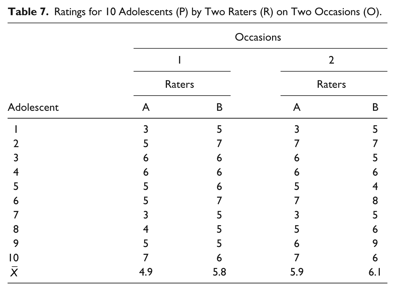
G-theory, however, handles this situation easily. Table 8 presents the estimates of the variance components for Table 7 data. Because the measurement involves object of measurement (P) and two facets (O, R), a three-way ANOVA model is called for. In this ANOVA model, there are three main effects (P, O, R), three two-way interactions (P*O, P*R, O*R), and one three-way interaction (P*O*R) confounded with error (e), due to insufficient degrees of freedom. Consequently, there are seven estimable variance components.

Table 8.

Variance Component Estimates for Table 8 Data.

Variance component	Estimate	%
$σ_{p}^{2}$	.61667	30.54
$σ_{o}^{2}$	.06111	3.02
$σ_{r}^{2}$	.23889	11.83
$σ_{p * o}^{2}$	.28889	14.31
$σ_{p * r}^{2}$	.31111	15.41
$σ_{o * r}^{2}$	−.02778⇒	.00
$σ_{p * r * o *, e}^{2}$	.50278	24.90

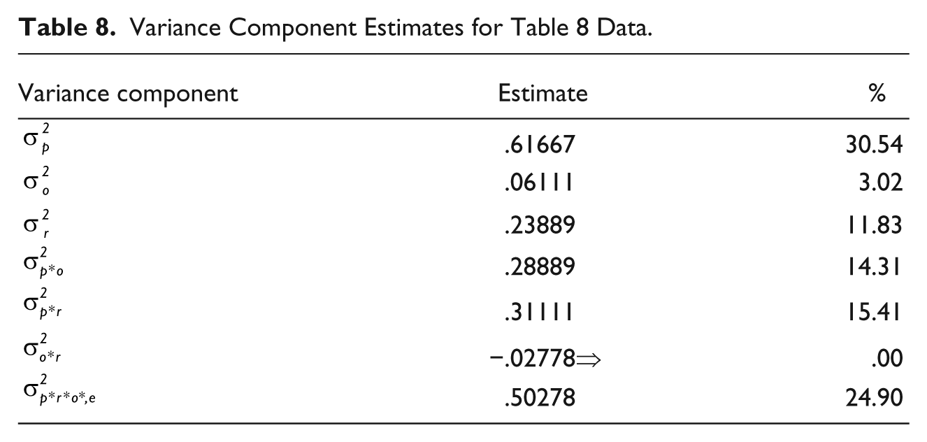
It is noted that the variance component for the object of measurement ( $σ_{p}^{2}$ ) constitutes about 31% of the total score variance, while 69% of total score variance being attributable to potential measurement error sources. There appears to be a nonnegligible rater effect ( $σ_{r}^{2}$ : 11.83%), indicating that the two raters differ in their ratings. As discussed before, the main effect of a facet only affects the absolute scores of the ratees but does not affect their relative positions. It is also noted that the two two-way interaction terms involving the object of measurement ( $σ_{p * o}^{2}$ , $σ_{p * r}^{2}$ ) are quite substantial, accounting for 14% and 15% of the total score variance, respectively. In addition, the three-way interaction term plus error is also substantial (25%). These interaction effects involving the object of measurement (P) affect the relative positions of the ratees. The two-way interaction between Occasion and Rater ( $σ_{o * r}^{2}$ ) does not involve the object of measurement (P), thus it will not affect the relative positions of the ratees but will only affect the absolute scores of the ratees.

Once these variance components are estimated, it is relatively easy to obtain the generalizability coefficients for Table 7 ratings based on two raters (n_r = 2) who provide ratings on two occasions (n_o = 2) for either relative or absolute decision. As discussed previously, relative decision G-coefficient is appropriate if we are only interested in the consistency of relative positions of the individuals. For relative decision G-coefficient, the error term includes all interaction components involving the object of measurement P:

\begin{array}{l} ρ^{2} = \frac{σ_{T}^{2}}{σ_{T}^{2} + σ_{E}^{2}} = \frac{σ_{p}^{2}}{σ_{p}^{2} + (\frac{σ_{p o}^{2}}{n_{o}} + \frac{σ_{p r}^{2}}{n_{r}} + \frac{σ_{p o r, e}^{2}}{n_{o} n_{r}})} \\ = \frac{. 61667}{. 61667 + \frac{. 28889}{2} + \frac{. 31111}{2} + \frac{. 50278}{4}} \\ = . 59 \end{array}

Absolute decision G-coefficient is appropriate when we are interested in the consistency of both relative positions and actual scores, and the error term includes all the components except the object of measurement P:

\begin{array}{l} φ = \frac{σ_{T}^{2}}{σ_{T}^{2} + σ_{E}^{2}} = \frac{σ_{p}^{2}}{σ_{p}^{2} + (\frac{σ_{o}^{2}}{n_{o}} + \frac{σ_{r}^{2}}{n_{r}} + \frac{σ_{p o}^{2}}{n_{o}} + \frac{σ_{p r}^{2}}{n_{r}} + \frac{σ_{o r}^{2}}{n_{o} n_{r}} + \frac{σ_{p o r, e}^{2}}{n_{o} n_{r}})} \\ = \frac{. 61667}{. 61667 + \frac{. 06111}{2} + \frac{. 23889}{2} + \frac{. 28889}{2} + \frac{. 31111}{2} + \frac{. 0000}{4} + \frac{. 50278}{4}} \\ = . 52 \end{array}

The φ coefficient above (φ = .52) is conceptually equivalent to intraclass correlation coefficient. Because ICC is not designed for this more complicated measurement situation, we cannot compute ICC for the data. We note that for the data in Table 7, measurement reliability involving two raters and two occasions appears to be low for both relative and absolute decisions. In a real measurement situation, we would be interested in improving the measurement process and measurement protocol to achieve better measurement reliability.

Improving the Measurement Process

The partitioning of the total score variance into multiple facets provides estimation of the percentage of variance attributable to each facet, and these variance components will help us understand the magnitudes measurement error from different error sources. For example, a relatively large variance component for the facet of Rater may suggest the need for better training for raters to achieve better consistency across raters. Similarly, a systematic interaction between Person and Rater indicates that the rater(s) are not applying consistent rating criteria to different ratees.

Planning for Measurement Reliability in Future Studies

Conventional reliability approaches are typically post hoc, that is, measurement reliability is computed after the fact.⁵ G-theory, however, is more proactive in planning for future measurement protocol. G-theory typically has two stages: G-study and D-study. The G-study serves as a “pilot” reliability study that provides information for planning the “real” research study. In the G-study, relevant variance components are estimated. In the D-study, the estimated variance components are used for planning for the measurement protocol of the “real” study so that the desired measurement reliability can be attained in the “real” study.

For example, for the J₁ vs. J₂’ data pair in Table 2, we previously (see Table 4) calculated Case 2 ICCs to be .61 (for J = 1) and .76 (for J = 2). Let’s assume that this is our “pilot” study (i.e., G-study), and we consider these reliability coefficients low and desire to attain higher measurement reliability in our “real” study. What should we do then?

In this case, we used J (J = 2) judges in our “pilot” study. If we consider ICC(2, J = 2) = .76 unacceptable, we may want to know what measurement reliability will likely to be if we increase the number of judges from two to four in our “real” study so that we may plan for our “real” study accordingly. This phase is called “D-study” in G-theory. D-study can be conducted regardless of norm-referenced or criterion-referenced score interpretation, and regardless of either a single facet (i.e., measurement error source) or multiple facets are involved in the measurement process.

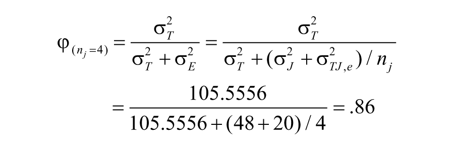
Using the variance components estimated for the data pair J₁ vs. J₂’ (Table 6), we can “forecast” the measurement reliability in our “real” study if we plan to use the mean of four⁶ judges’ rating for each target (person), and this involves the simple substitution of n_j = 4 in the equation for G-coefficient for absolute decision as shown below. If we consider φ = .85 satisfactory for our purpose of study, we may plan to conduct our “real” study by using four judges to rate each target (person) and use the mean of the four judges as the rating for each target (person).

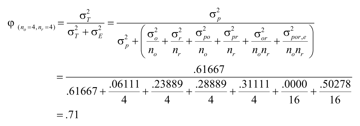
\begin{array}{l} φ_{(n_{j} = 4)} = \frac{σ_{T}^{2}}{σ_{T}^{2} + σ_{E}^{2}} = \frac{σ_{T}^{2}}{σ_{T}^{2} + (σ_{J}^{2} + σ_{T J, e}^{2}) / n_{j}} \\ = \frac{105.5556}{105.5556 + (48 + 20) / 4} = . 86 \end{array}

In the same vein, for the two-facet (rater and occasion) measurement data in Table 7, we previously estimated all relevant variance components (Table 8) and calculated G-coefficient for absolute decision for the mean rating based on two raters and two occasions (φ = .52). We may desire to attain higher measurement reliability in our “real” study by either increasing the number of raters, the number of occasions, or both (assuming that practical constraints, such as cost, time, etc., allow us to do so). As an illustration, we may consider a measurement scenario of using four occasions and four raters (n₀ = 4, n_r = 4):

\begin{array}{l} φ_{(n_{o} = 4, n_{r} = 4)} = \frac{σ_{T}^{2}}{σ_{T}^{2} + σ_{E}^{2}} = \frac{σ_{p}^{2}}{σ_{p}^{2} + (\frac{σ_{o}^{2}}{n_{o}} + \frac{σ_{r}^{2}}{n_{r}} + \frac{σ_{p o}^{2}}{n_{o}} + \frac{σ_{p r}^{2}}{n_{r}} + \frac{σ_{o r}^{2}}{n_{o} n_{r}} + \frac{σ_{p o r, e}^{2}}{n_{o} n_{r}})} \\ = \frac{. 61667}{. 61667 + \frac{. 06111}{4} + \frac{. 23889}{4} + \frac{. 28889}{4} + \frac{. 31111}{4} + \frac{. 0000}{16} + \frac{. 50278}{16}} \\ = . 71 \end{array}

These D-studies for different measurement scenarios allow us to assess the impact of changing measurement conditions on measurement reliability, thus allowing us to design the optimal measurement protocol (considering measurement reliability, cost, time, other practical constraints) for our “real” research study. This aspect of G-theory provides researchers with the flexibility and forecasting capability that are not previously available in conventional reliability approaches.

Conclusions

In this article, we discussed that some adolescence researchers’ understanding of measurement reliability may be fragmented, and it is not always clear how different reliability coefficients are related. We have shown that generalizability theory (G-theory) is a comprehensive framework of measurement reliability, and this framework subsumes all other reliability methods (e.g., reliability coefficients based on Pearson r, coefficient alpha and KR-20, intraclass correlation coefficients). As such, G-theory provides the degree of flexibility and comprehensiveness not offered by the conventional approaches. Within the G-theory framework, the similarities and differences of different reliability coefficients can be easily understood, and planning for optimal measurement protocols becomes feasible. Adolescence researchers may move beyond the fragmented treatment of measurement reliability and consider and use generalizability theory as the general framework for different reliability estimates in their substantive studies.

Footnotes

Declaration of Conflicting Interests

The author(s) declared no potential conflicts of interest with respect to the research, authorship, and/or publication of this article.

Funding

The author(s) received no financial support for the research, authorship, and/or publication of this article.

Notes

Author Biographies

Xitao Fan is dean and chair professor, University of Macau, China. Previously, he was in Utah State University, and University of Virginia, USA. He focuses on applications of quantitative methods in educational/psychological research, with many well-cited publications in a variety of educational/psychological journals. He is an AERA Fellow (2012).

Shaojing Sun is an associate professor in communication, Fudan University, China. With PhD degrees from both Kent State University and University of Virginia, he focuses on applications of quantitative methods in communication research. He has published numerous refereed articles in journals in communication, education, psychology, marketing, and public health.

References

Algina

(1978). Comment on Bartko’s “On various intraclass correlation reliability coefficients.” Psychological Bulletin, 85, 135-138. doi:10.1037/0033-2909.85.1.135

Bartko

J. J.

(1966). The intraclass correlation coefficient as a measure of reliability. Psychological Reports, 19, 3-11. doi:10.2466/pr0.1966.19.1.3

Bartko

J. J.

(1976). On various intraclass correlation reliability coefficients. Psychological Bulletin, 83, 762-765. doi:10.1037/0033-2909.83.5.762

Bartko

J. J.

(1978a). Reply to Ronald A. Berk: On Bartko’s intraclass correlations of interrater reliability. Perceptual & Motor Skills, 47, 721-722. doi:10.2466/pms.1978.47.3.721

Bartko

J. J.

(1978b). Reply to Algina. Psychological Bulletin, 85, 139-140. doi:10.1037/0033-2909.85.1.139

Brennan

R. L.

(2006). Educational measurement (4th ed.). New York, NY: Rowman & Littlefield.

Brennan

R. L.

(2010). Generalizability theory. New York, NY: Springer.

Brown

K. W.

West

A. M.

Loverich

T. M.

Biegel

G. M.

(2011). Assessing adolescent mindfulness: Validation of an adapted mindful attention awareness scale in adolescent normative and psychiatric populations. Psychological Assessment, 23, 1023-1033. doi:10.1037/a0021338

Cardinet

Johnson

Pini

(2009). Applying generalizability theory using EduG. New York, NY: Routledge.

10.

Cicchetti

D. V.

(1994). Guidelines, criteria, and rules of thumb for evaluating normed and standardized assessment instruments in psychology. Psychological Assessment, 6, 284-290. doi:10.1037/1040-3590.6.4.284

11.

Crocker

Algina

(1986). Introduction to classical and modern test theory. Fort Worth, TX: Holt, Rinehart and Winston.

12.

Cronbach

L. J.

(1951). Coefficient alpha and the internal structure of tests. Psychometrika, 16, 297-334. doi:10.1007/BF02310555

13.

Cronbach

L. J.

Gleser

G. C.

Nanda

Rajaratnam

(1972). The dependability of behavioral measurement. New York, NY: John Wiley.

14.

Gulliksen

(1987). Theory of mental tests. Hillsdale, NJ: Lawrence Erlbaum.

15.

Hoyt

C. J.

(1941). Test reliability estimated by analysis of variance. Psychometrika, 6, 153-160. doi:10.1007/BF02289270

16.

Kuder

G. F.

Richardson

M. W.

(1937). The theory of the estimation of test reliability. Psychometrika. 2, 151-160. doi:10.1007/BF02288391

17.

Maisto

S. A.

Krenek

Chung

Martin

C. S.

Clark

Cornelius

(2011). A comparison of the concurrent and predictive validity of three measures of readiness to change alcohol use in a clinical sample of adolescents. Psychological Assessment, 23, 983-994. doi:10.1037/a0024136

18.

McDonald

R. P.

(1999). Test theory: A unified approach. Mahwah, NJ: Lawrence Erlbaum.

19.

McGraw

K. O.

Wong

S. P.

(1996). Forming inferences about some intraclass correlations coefficients: Correction. Psychological Methods, 1, 390. doi:10.1037/1082-989X.1.4.390

20.

Shavelson

R. J.

Webb

N. M.

(1991). Generalizability theory: A primer. Thousand Oaks, CA: Sage.

21.

Shrout

P. E.

Fleiss

J. L.

(1979). Intraclass correlations: Uses in assessing rater reliability. Psychological Bulletin, 86, 420-428. doi:10.1037/0033-2909.86.2.420

22.

Traub

R. E.

(1994). Reliability for the social sciences: Theory and applications. Thousand Oaks, CA: Sage.

23.

Valen

Ryum

Svartberg

Stiles

T. C.

McCullough

(2011). The achievement of therapeutic objectives scale: Interrater reliability and sensitivity to change in short-term dynamic psychotherapy and cognitive therapy. Psychological Assessment, 23, 848-855. doi:10.1037/a0023649

24.

Wilkinson

, & the Task Force on Statistical Inference. (1999). Statistical methods in psychology journals: Guidelines and explanations. American Psychologist, 54, 594-604. doi:10.1037/0003-066X.54.8.594

25.

Worthen

B. R.

White

K. R.

Fan

Sudweeks

R. R.

(1999). Measurement and assessment in schools (2nd ed.). New York, NY: Allyn & Bacon/Longman.

Supplementary Material

Please find the following supplemental material available below.

For Open Access articles published under a Creative Commons License, all supplemental material carries the same license as the article it is associated with.

For non-Open Access articles published, all supplemental material carries a non-exclusive license, and permission requests for re-use of supplemental material or any part of supplemental material shall be sent directly to the copyright owner as specified in the copyright notice associated with the article.

0.52 MB

0.00 MB

0.25 MB