
Abstract
We propose the use of archetypes as a way of moving between conceptual framings, empirical observations and the dichotomous classification rules upon which maps are based. An archetype is a conceptualisation of an entire category or class of objects. Archetypes can be framed as abstract exemplars of classes, conceptual models linking form and process and/or tacit mental models similar to those used by field scientists to identify and describe landforms, soils and/or units of vegetation. Archetypes can be existing taxonomic or landscape units or may involve new combinations of landscape attributes developed for a specific purpose. As landscapes themselves defy precise categorisation, archetypes, as considered here, are deliberately vague, and are described in general terms rather than in terms of the details that characterise a particular instance of a class. An example outlining the use of archetypes for landscape classification and mapping is demonstrated for granitic catenas in Kruger National Park, South Africa. Some 81% of the study area can be described in terms of archetypal catenal elements. However, spatial clustering of two classes that did not correspond to the archetypes prompted development of new archetypes. We show how the archetypes encoded in the map can be used to frame further knowledge in an ongoing, iterative and adaptive process. Building on this, we reflect on the value of vagueness in conservation science and management, highlighting how archetypes that are used to interpret and map landscapes may be better employed in the future.
Keywords
I Introduction
All maps are underpinned by a conceptual model of the world (e.g. Crampton, 2001). Ecological maps are generally either ‘bio-ecological’ or ‘geo-ecological’ (Moss, 2000). Whereas the ‘bioecological’ perspective focusses on particular organisms and their habitats (e.g. Wiens, 1989), the ‘geo-ecological’ perspective is based largely on relationships between vegetation, soils and topography, perceived as forming a mosaic of landscape patches, each of which is capable of supporting a certain range of organisms (e.g. Bailey, 2009). Here we focus on ecological mapping from the geo-ecological perspective, exploring relationships between the conceptual models used to describe and explain ecological patterns or to partition landscapes into management units and approaches to mapping these patterns.
We advocate the use of archetypes as an approach that allows users to move between theoretical framings, empirical observations and the classification rules upon which ecological maps and management plans are based. Our approach builds upon a previous study (Cullum et al., 2016) that outlines how the selection of scales and attributes for ecological classification and mapping needs to be informed by a conceptual framework that is supported by narratives that demonstrate its relevance and credibility for particular purposes (Cash et al., 2003). Here we focus on the central role of archetypes in the construction of such conceptual frameworks.
Although landscapes and the elements that comprise them are not necessarily discrete or well bounded in space or time (Fisher et al., 2004; Richards and Clifford, 2011), each spatio-temporal location is potentially unique (Phillips, 2007) and ecological surprises (Holling, 1986; Lindenmayer et al., 2010) are to be expected, recurring spatial and temporal patterns can be observed in most landscapes, across many scales. Such patterns and relationships are not entirely predictable, but neither are they haphazard (e.g. Kay and Schneider, 1994). As Mitchell (2009: 105–106) puts it: We do not live in Heraclitus’s ever changing and unknowable world of eternal flux. But neither do we live in Parmenides’ world of the unchanging, where only the eternal is knowable [see Kirk et al., 1983]. Instead we live in a world that comes in many shapes and sizes with structures differing in degrees of stability, affording more or less contingent truths that we can know and use to pursue our goals and aspirations.
When seeking to describe, understand or manage the world, we are forced to generalise and abstract our observations and experience by categorising space into structural-functional units that are based on our perceptions of such regularities and structures. Each of these units represents an area characterised by a cluster of interdependent biophysical entities and processes, shaped by a history of human activity and natural events. Each unit can be related to a ‘process domain’ (Delcourt et al., 1982; Montgomery, 1999), in which certain key processes control the behaviour of the unit, generating and sustaining characteristic features and attributes.
Geo-ecological landscape units can be defined at many scales and viewed from many perspectives. Examples at various scales from different disciplines include hydrological response units (Flugel, 1995), pedons (e.g. Huggett, 1975), landforms or river reaches (e.g. Brierley and Fryirs, 2005) and plant communities (e.g. Braun-Blanquet, 1928). In each case, characteristics of the whole unit define it from a particular perspective. For example, patterns in topography and vegetation inform soil and hydrological mapping, since these patterns are known to covary with both soil and hydrology (e.g. Milne, 1935). Similarly, distributions of plant species and communities are often described and mapped in terms of covarying abiotic attributes such as temperature, precipitation, substrate or aspect (Whittaker, 1956). The similarity of the areas defined by different disciplines arises from both the interdependency and co-evolution of many types of entities and processes and from context-dependent constraints on a wide range of biological, physical, chemical and social processes.
The categorisation of the Earth’s surface into geo-ecological landscape units provides a way to simplify the complexity of form and function, providing vital contextual information to support land and water management and policy initiatives. Particular features and/or attributes provide the basis for classifications that aim to reflect differences in the processes that generate and sustain observed patterns. Such frameworks inform the selection of sample and monitoring sites and facilitate the meaningful transfer of understanding between different locations. The rationale for extrapolation between locations is based on the assumption that the same processes shape units in the same category and that these processes are subject to the same drivers and constraints in a particular category. Thus, similar forms and behaviour are to be expected in all locations that belong to the same class. Although these assumptions may not hold equally true for all class members, and in some cases a completely different set of processes may have generated the observed features (the principle of equifinality or convergence, see Beven, 2002), the imperfection of classification is tolerated, provided that the classification provides sufficient general knowledge to be useful for a particular application. The degree of imperfection that is tolerable depends on the needs and aspirations of end users, who must inevitably trade-off classification imperfections against the utility of generalisation.
Despite the widespread use of landscape categorisations, there is no standard approach to the delineation of such units, either within or between disciplines. There is no single way of ‘carving nature at its joints’ (Plato, Pheadrus: 265e, 1997). Instead, there are many ways of viewing and partitioning any particular landscape. Different patterns and processes can be observed, depending on the scale of observation (Levin, 1992; Wiens, 1989), the attributes that are considered and the variables used to describe them (e.g. Buyantuyev and Wu, 2007). Landscape classifications thus reflect established institutional and disciplinary perspectives, with varying levels of importance and relevance given to different scales and attributes in different disciplines, management agencies and applications (Benda et al., 2004; Boulton et al., 2008; Tadaki et al., 2012).
Furthermore, local differences may prevent the implementation of standard, universally applicable classifications, since the combination and relative importance of factors that influence patch character and behaviour vary in space and time (e.g. Brierley et al., 2013; Grayson and Bloschl, 2000; Omernik, 2004; Ridolfi et al., 2003; Rodriguez-Iturbe, 2000; Scull et al., 2003). It is often appropriate to split or clump classes in different ways in different settings, since subtle variations that may be disregarded in one location can be important local differences elsewhere. For example, aspect may be an important determinant of vegetation patterns in one place, but in another, slope or elevation may be far more important (Omernik, 2004). Furthermore, many landscapes contain ‘unusual’ features and processes that are absent or rare elsewhere but are important to that specific context (Brierley and Fryirs, 2000). Thus, standardised classifications that are intended to be universally applicable can omit or downplay site-specific or historical factors that are locally important in driving or controlling the processes of interest (Simon et al., 2007).
The advent of widely available, high-resolution remotely sensed data and other ‘big data’ offers users tantalising opportunities for more objective landscape classifications (Brasington et al., 2012; Hampton et al., 2013; Peters et al., 2014; Sellars et al., 2013; Wheaton et al., 2015). However, the counterargument is that ‘big data’ vastly multiplies the opportunities for viewing landscapes at different scales and from many different perspectives. How then, do we decide which scales and attributes are most useful for a particular purpose? How can we rationalise and evaluate approaches to integrated catchment management, national conservation plans or setting global conservation priorities (see, for example, Abell et al., 2008; Driver et al., 2005; Kleynhans et al., 2005; Olson et al., 2001)? We contend that landscape archetypes potentially provide an important building block for such endeavours.
An archetype is a conceptualisation of an entire category or class of objects, framed as an abstract exemplar of the class. Archetypes describe patterns of form and process in abstract, general terms rather than with the precise details that characterise a particular instance of a class. We suggest that such imprecision is a virtue rather than a hindrance, well suited to describing landscapes that are themselves inherently imprecise. Our notion of an archetype is based upon Rosch’s prototype theory of categories, which describes cognitive and semantic classification in terms of graded class membership (Rosch, 1975, 1978). The degree of class membership is determined by the degree of similarity to one or more class exemplars or ‘prototypes’ that portray an idealised class member. We move from cognitive and semantic classification into the realms of fuzzy logic and fuzzy classification techniques (Burrough, 1989; Zadeh, 1965) and the tacit mental models that are used to identify and describe landforms, soils and patches of vegetation (Bui, 2004). We suggest that archetypes provide useful ways of articulating the assumptions underlying geo-ecological classifications and maps, guiding the selection of scales and variables. We demonstrate how the use of archetypes informs fuzzy classifications that integrate object (categorical) and gradient (continuous) views of the world, allowing categorical groupings that retain information about local differences that may turn out to be important, while also providing a rationale for generalisations upon which spatial extrapolations can be based.
The structure of the paper is as follows. We start by introducing the concept of landscape archetypes, considering how they can be derived and used in landscape classification and mapping and developing an example for the granitic catenas in Kruger National Park (KNP), South Africa. We then consider how the archetypes encoded in the map can be used to frame further knowledge in an ongoing, iterative and adaptive manner. Lastly, we reflect on the value of vagueness in conservation science and management and we discuss how a deeper understanding of archetypes can inform the mapping and interpretation of landscapes.
II The inherent vagueness of landscape units
Inevitably, the conceptualisations that frame scientific understandings of landscapes are human constructions and are, therefore, provisional and subject to revision (Church, 1996; Pickett et al., 2007; Popper, 1959; Wohl et al., 2005). The conceptualisations can be considered in terms of the semiotic triangle, which considers relationships between our thoughts (conceptualisations) of the world (reality) and representations thereof (Ogden and Richards, 1923, Figure 1). In cartography, for example, maps are perceived as realities created through a relationship between the mapmaker, the map reader and the medium in which the map is portrayed (e.g. Crampton, 2010; Kitchin et al., 2013). Here we contend that archetypes can mediate between all points of the semiotic triangle, facilitating user consensus around conceptualisations and maps of landscapes that that they find useful for particular purposes.
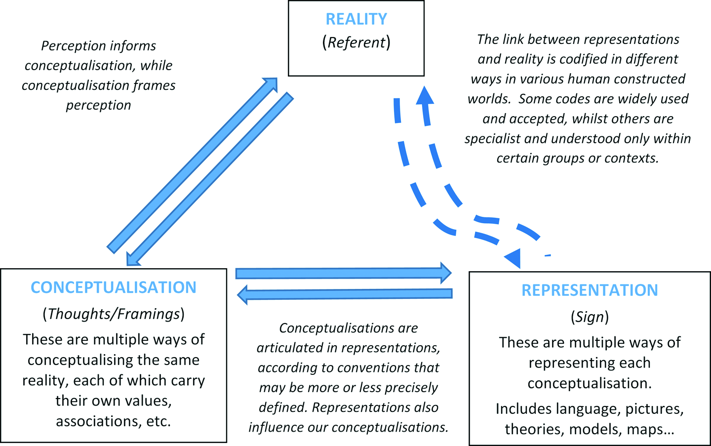
Relationships between reality, conceptualisations and representations. Conceptualisations of reality can be articulated and shared in many representations. Relationships between reality, conceptualisations and representations mirror the semiotic triangle in which signs and symbols (representations) stand for thoughts (conceptualisations) about referents (reality) (after Ogden and Richards, 1923).
One of the central challenges in defining and mapping landscape units that describe spatial clusters of biophysical attributes is that all three points of the semiotic triangle are inherently vague: The referent (a landscape) is itself inherently imprecise. For example, river reaches, vegetation patches and landforms generally have indeterminate positional and class boundaries: Where does a mountain or a patch of soil or vegetation or a river landform begin and end (Burrough, 1989; Burrough and Frank, 1996; Fisher et al., 2004; Wheaton et al., 2015)? Furthermore, landscapes are dynamic, such that boundaries are often fluid in space and time. There are also many local exceptions to observed recurrences in form and process (Beven, 1999; Phillips, 2007; Richards and Clifford, 2011; Wohl, 2013). Our perceptions of landscape entities also vary with context. For example, patches may appear or disappear and boundaries appear more precisely delineated when observed at finer grains (Fisher, 2000; Wiens, 1989). Perceptions are also limited by data availability and knowledge (e.g. satellite imagery, soil maps and climate data may be available for some areas, but not others, or show only selected ecological attributes). The various conceptualisations used to describe landscape entities are vague, possibly ambiguous and certainly contestable. Since the human mind is limited in the number of ideas it can hold simultaneously, all mental concepts of landscapes are necessarily abstractions and generalisations that simplify and emphasise particular perspectives. There are many subtle variations of the same concepts, which together form a cluster of slightly overlapping meanings, so that we cannot say exactly what meanings are included or excluded: What is a forest? What constitutes a wetland? (e.g. Bennett, 2001; Rosch, 1975). Further vagueness arises from perspectives that emphasise different attributes of the same entity. For example, roads can be conceptualised in terms of their physical characteristics, function in transportation, legal status, geographic position and degree of influence on the adjoining landscape (Fisher, 2000). The representation of these concepts in models (including language, diagrams and maps) is also inherently vague, since the degree of realism, generality and precision depends on trade-offs in representation between generality, precision and realism (see Levins, 1966). The mode of presentation also limits possibilities; for example, paper maps can only represent two dimensions and a snapshot in time. Many linguistic concepts reflect underlying conceptual vagueness, as illustrated by the Sorites paradox, in which there is no threshold at which the addition or removal of single grains creates or destroys a ‘heap’ of sand (described in Bennett, 2005; Fisher, 2000; Regan et al., 2002).
We propose the use of archetypes and fuzzy logic as a way of addressing the challenges (and opportunities) presented by this vagueness.
III Archetypes and fuzzy logic
1 What is a landscape archetype?
Landscape archetypes can be conceived and represented in many ways: they can be real examples of landscape units, abstract mental constructs, theoretical concepts or textbook examples. The most useful archetypes for landscape management and science inform both explanatory conceptual models that link form and process and rules for the delineation and mapping of landscape units and classes. Such archetypes can provide a rationale for the spatial extrapolation of expected behaviour and responses to management initiatives, thereby providing a sound basis for the selection of sites for long-term monitoring, observation or experiment.
Rosch’s prototype theory of categories (Rosch, 1975, 1978) challenges the classical, Aristotelian approach to classification in which cognitive and semantic categories are defined in terms of necessary and sufficient conditions that can be translated into rules that define each class. According to the classical approach, the world is divided into ‘natural kinds’ that are individually mutually exclusive and collectively exhaustive. Each of these natural categories or classes is bounded by rules that describe the binary yes/no conditions for class membership. Furthermore, all class members are considered to be interchangeable, so that any randomly selected class member represents the whole class equally as well as any other class member.
Rosch (1975, 1978) demonstrated that the classical approach offers a limited view of cognitive and semantic classification. Many of the groups we commonly refer to in language are based upon vague ‘family resemblances’ (Wittgenstein, 1953), rather than on fixed rules. Members of classes based on family resemblance tend to share properties with each other, but no single property or set of properties is either necessary or sufficient for class membership. Thus, some members may have a certain property (to a greater or lesser extent), while others lack it but exhibit other properties that are also typical of the class. Building on this idea, Rosch suggested that class membership can be graded, determined by the degree of similarity to one or more class exemplars or ‘prototypes’ that portray an idealised class member. Thus, some class members are more similar to the prototype(s) than others and are consequently seen as better representatives of the whole class. For example, in the classical approach to classification, a bird is defined as having a certain set of characteristics (e.g. an animal with feathers, a beak and the ability to fly) and all animals are then classified as either ‘bird’ or ‘not bird’. By contrast, using a prototype approach (or in general parlance), a robin could be considered to be a more typical example of a bird (or closer to the ‘bird’ prototype) than a kiwi, which cannot fly, but is nevertheless a legitimate member of the class ‘bird’ (Rosch, 1975).
We use the term ‘archetype’ rather than ‘prototype’ because the secondary meanings of the word ‘prototype’ impart overtones of an early, undeveloped, tangible model. Furthermore, we do not want to suggest that prototypical ‘natural categories’ exist that are ‘more rapidly learned and more often chosen’ (Rosch, 1973: 328) than other categories into which landscapes can be partitioned. Instead, we conceive archetypes as mental constructs or theoretical artefacts that may be tacit, but can also be carefully constructed, challenged, refined and adapted to suit local circumstances and particular purposes. Furthermore, the term archetype has previously been used to describe classes of landscape units at various scales (e.g. Sommer and Schlichting, 1997; Václavík et al., 2013).
Whereas prototype theory was designed to explain unconscious cognitive and learning processes and semantic classifications, it can also be reverse engineered to build mental models and classification schemes. Indeed, prototype theory and the use of landscape archetypes are closely related to fuzzy set theory, fuzzy logic and techniques of fuzzy classification. These mathematical and computational tools address vagueness, mediating between natural language, precise information ontologies and the blurriness of the natural world (e.g. Burrough, 1989; MacMillan et al., 2000; Qi et al., 2006; Qin et al., 2009). As Burrough (1989: 491) explains: The strength of the fuzzy set approach is that it starts from the premise that nature may be inherently vague or imprecise, and does not try to pretend that the real world, which has been modelled by data entities created by human or machine observation, is more exact, or more perfect than it really is.
IV Reasoning with fuzzy logic
Traditional approaches to scientific discourse and enquiry demand precision and conceptual clarity, relegating vague concepts and statements to the realm of pseudo-science and belief (Strunz, 2012). Whereas the scientific method involves rigorous testing of precisely articulated hypotheses that are designed to separate potential truth from falsehood or nonsense (Popper, 1959), vagueness allows for partial truths that cannot be rigorously tested, since concepts can shift to accommodate reality (Zadeh, 1996). As noted earlier, however, scientific understanding is inherently provisional, mediated between conceptualisations and representations in the way we see ‘reality’ (Figure 1).
Zadeh (1996, 2008) neatly mathematically formalises how we communicate and reason in shades of grey rather than in black and white, and how fuzzy linguistic variables that can enclose various degrees of size, value, truth and possibility can describe our inherently fuzzy world far better than can bivalent variables: Fuzzy logic is not fuzzy. Basically, fuzzy logic is a precise logic of imprecision and approximate reasoning. More specifically, fuzzy logic may be viewed as an attempt at formalization/mechanization of two remarkable human capabilities. First, the capability to converse, reason and make rational decisions in an environment of imprecision, uncertainty, incompleteness of information, conflicting information, partiality of truth and partiality of possibility – in short, in an environment of imperfect information. And second, the capability to perform a wide variety of physical and mental tasks without any measurements and any computations. (Zadeh, 2008: 2751) Granulation is a form of information compression, in which a fuzzily defined range of values is reduced to a single granule, defined as ‘a clump of attribute-values drawn together by indistinguishability, similarity, proximity or functionality’ (Zadeh, 2008: 2754). Applied to landscape units, this term describes how we conceptually decompose landscapes into granular clusters of environmental features and/or attributes. Features and attributes are aggregated in terms of their similarity, proximity, functionality, suitability for purpose or in terms of some other criterion. Often, these clumps are arranged vertically and horizontally in a hierarchy (Allen and Starr, 1982). Precisiation is a process in which an object progressively becomes more precisely defined, either in terms of meaning or value (in the mathematical, not the normative sense of the word). We use a process of precisiation when we move from the general to the particular, either by employing a finer scale of observation and/or applying generalised abstractions to a particular location or instance of a category. Conversely, the reverse process of ‘imprecisiation’ allows summaries, comparisons and extrapolations across space and time. Movements between the general to the particular are always problematic and carry a heavy cost (e.g. Burt, 2005; Cushman et al., 2010a; Wu, 2004). Generalised constraints are limitations on possibility, probability or notional truth. This concept is echoed in hierarchy theory, in which landscape units at higher organisational levels are conceived as contextual constraints on the forms and processes found in units at lower organisational levels (Allen and Starr, 1982; Phillips, 2004). Conversely, landscape units at lower hierarchical levels also shape possibilities at higher levels. Graduation means that everything is allowed to be a matter of degree (or ‘fuzzy’). Such approximation and vagueness is well suited to landscape analyses, where boundaries are blurred and locations are unique, such that models do not fit perfectly everywhere (Phillips, 2007). Fuzzy classification techniques accommodate graduation by using membership functions that define the degree to which a particular unit fits the criteria for a class, rather than by merely assigning a binary ‘yes/no’ class membership (see discussion and Figure 2 below). Generalised constraints can relate to possibility, probability or notional truth. This concept is echoed in hierarchy theory, in which landscape units at higher organisational levels are conceived as contextual constraints on the forms and processes found in units at lower organisational levels (Allen and Starr, 1982; Phillips, 2004).
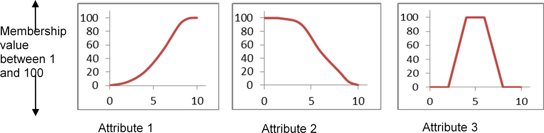
Fuzzy classification. Membership functions describe the relationship between an archetype and each of its defining attributes. The attributes of a pixel (or group of pixels) are compared to these functions to derive a membership value that describes the similarity between the pixel and the archetypal class, expressed as a degree of class membership. Multiple attributes can be considered and a composite membership value obtained by aggregating the results, usually by using either weighted or unweighted means (see Burrough, 1989).
Fuzzy classification is now routinely used in classifications derived from remotely sensed imagery (e.g. Foody, 1996) and mapping applications, such as digital soil mapping (e.g. Burrough, 1989), geomorphic mapping (e.g. Fisher et al., 2004) and vegetation mapping (e.g. Roberts, 1996). Here we seek to extend these applications using landscape archetypes viewed as fuzzy, abstract entities. Each granule that a landscape is partitioned into can, more or less precisely, be described in terms of an archetype. The archetype itself can have fuzzy (graduated) boundaries, and the degree to which particular tracts of land are similar to an archetype can be assessed. The extent to which dynamics and behaviour follow the archetype can also vary between locations.
V How archetypes are constructed and used in the classification and mapping of landscape units
Archetypes are heuristic abstractions that serve as a starting point for the description of a landscape. If there are multiple valid ways of describing a landscape, and hence multiple archetypes upon which ecological classification and maps for a particular area might be based, how can we determine the most useful archetype(s) for a particular purpose? Furthermore, how can we produce an integrated classification or map that is relevant and useful to diverse stakeholders? Consensus is required around a conceptualisation that identifies landscape objects and processes of interest, in terms of their classes and scales (including grain and extent). Indeed, the lack of a shared framework and consequent mismatches of scale and/or geographic foci often lies behind the failure of transdisciplinary projects and hinders the application of scientific knowledge to management applications (Dollar et al., 2007; Pickett et al., 2007). A shared framework may be detailed and precise, incorporating details of features and processes pertinent to a specialist perspective. More commonly perhaps, framings are vague and imprecise, providing aligned contextual information about landscapes that integrates the various points of view of scientists and managers working on the same landscapes from the perspectives of different disciplines and institutions (Stirzaker et al., 2011). Explicit narratives that justify and legitimise the adoption of a shared conceptualisation provide transparency that not only allows conceptualisations to be contested, but also allows archetypes to be refined as new knowledge and experience is gained (i.e. adaptive management or ‘learning through doing’; Holling, 1978). Conceptualisations of landscape entities and archetypes provide a platform for such investigations and applications.
1 Constructing a landscape archetype
Starting points for the construction of landscape archetypes can be process-based or phenomenological, based either on real examples, on existing taxonomies or classifications, or on inductive pattern analysis. Process-based approaches entail the description of an idealised abstraction of the central tendencies of a class, linking observed features to hypothesised generative mechanisms. Although it is not always possible to describe the detailed mechanisms responsible for a particular biophysical pattern, idealised conceptual models describe the broad character and behaviour of many geo-ecological phenomena, relating diagnostic characteristics of specific landscape features to formative processes and contemporary behaviour. Such models not only provide a basis for spatial extrapolation and forecasting the likely future behaviour of different landscape classes under various scenarios, but also lend credibility to the classification itself. Process-based approaches to the construction of a landscape archetype might start from a well-established conceptual model that describes the processes, drivers and controls that generate observable features and patterns. Alternatively, these models might be adapted to apply to a particular landscape, as in the tacit mental models used by soil surveyors and geomorphologists when they are ‘reading the landscape’ (Fryirs and Brierley, 2012; Qi et al., 2008). Process-based conceptualisations can also be constructed by synthesising local knowledge and experience with broader scientific theory (e.g. Lane et al., 2011; Wilcock et al., 2013).
Although process-based archetypes are usually preferable, where mechanisms are contested or poorly understood, archetypes can be purely empirical. Phenomenological approaches can involve the description of a real example, carefully selected to be the most representative examples of a predetermined class, displaying all the features and properties that are most commonly associated with the class. This approach is analogous to the use of training samples in supervised statistical classification. Like the process-based approach, this way of constructing archetypes relies upon the a priori, abstract definition of classes but recognises them solely via shared pattern characteristics. Such definitions can involve combinations of existing taxonomic classes or mapping units. For example, combinations of existing soil series, vegetation classes, river topologies and landforms may prove a useful starting point for the development of archetypal landscape units.
Statistical pattern analyses aim to reveal patterns in data. Although designed to remove observer bias, such bias is inescapable, since all analysis is constrained by the availability and/or selection of data inputs and the chosen methods and scale(s) of analysis (see Blue and Brierley, 2016). Such unsupervised classifications may reveal subtle patterns that are not easily detected by visual inspection alone. However, comparisons and extrapolations of patterns could be misleading if classes group together spatial objects formed by different processes, prospectively with different evolutionary trajectories. Furthermore, patterns may reflect one-off correlations, which do not recur systematically and cannot be related to generative processes. Nevertheless, observed similarities in the character of landscape patches can suggest hypotheses about why the objects are similar, how the perceived order has come to exist and whether or not it will persist (Sokal, 1974).
In practice, process-based and empirical approaches to defining archetypes overlap. For example, a textbook conceptual model might identify the key attributes that are likely to be spatially aligned and statistical procedures may be used to assess the factors most strongly aligned in a particular landscape of interest. This analysis might then stimulate new insights, adding new dimensions to the conceptual model. Alternatively, in situations where no conceptual model exists or no expert knowledge is available (or different experts offer contested opinions), the interplay might start with a statistical description of spatial clusters of selected environmental attributes. Once an archetype has been constructed, the next challenge is to operationalise the conceptual model, using it as the basis for an a priori landscape classification.
2 Representing landscape archetypes in a map
Representing conceptual archetypes in a map involves determining the scales of interest, partitioning a landscape into units and grouping these units into classes associated with each archetype. This process involves the construction of a semantic import model, in which concepts embedded in the language, theory and/or tacit mental models of experts are translated into rules that can be encoded in a computerised mapping procedure (e.g. Bui, 2004; Burrough, 1989; Hengl and MacMillan, 2009; Walter et al., 2006). Several sets of rules may be used to represent the same archetype, since different attributes may be associated with the same landscape archetype observed in different imagery, at different times of the year or following disturbances such as fire or flood. Probabilistic classification techniques are well suited to this task, since both the semantic models and the landscapes themselves are rarely precise or have abrupt boundaries. Most classification methods can evaluate the probability of class membership being correctly assigned (e.g. Classification and Regression Tree [CART], neural networks), while others can start from the premise that the classes themselves are imprecise (e.g. Bayesian and fuzzy classification techniques). Here, we focus on fuzzy classification approaches.
In fuzzy classification, the degree to which an object is similar to a pre-defined example is defined using membership functions that are based on fuzzy set theory (Zadeh, 1965). Similarity is assessed using multiple characteristics, each of which is described in terms of membership functions that specify the relationship between an observed value of each attribute and the degree of class membership associated with this value (Figure 2). The values associated with different attributes are then combined to produce an overall membership value. For example, an archetype of the class ‘gravel bed stream’ could be described as occurring at the bottom of a hillslope, with a concave profile curvature and containing particles that measure between x and y cm across their intermediate axis. Membership functions could then be constructed for each of these attributes and their values (weight) averaged to derive an overall class membership value.
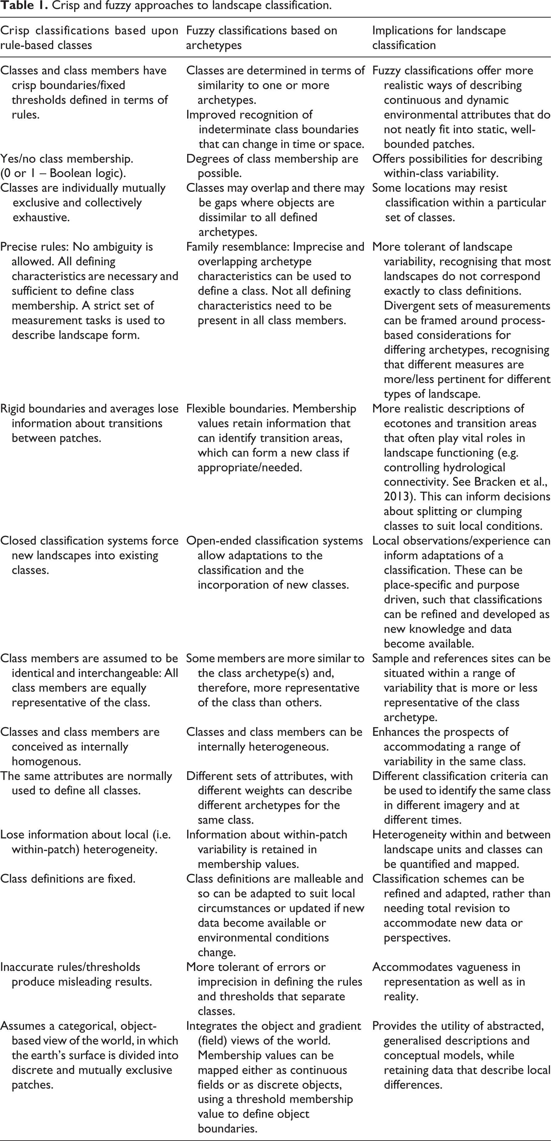
Whereas crisp classification techniques require unambiguous and exclusory definitions for each category, yielding sharply defined boundaries and mutually exclusive classes, fuzzy classification techniques tolerate continuous/blurred classes and positionally vague boundaries (Table 1). While conventional rule-based approaches to landscape classification focus attention on the definition of boundaries, archetype-based approaches focus attention on the core attributes that characterise a cluster of environmental variables.
Crisp and fuzzy approaches to landscape classification.
VI An example of archetype construction and representation: mapping granite catenas in Kruger National Park (KNP), South Africa
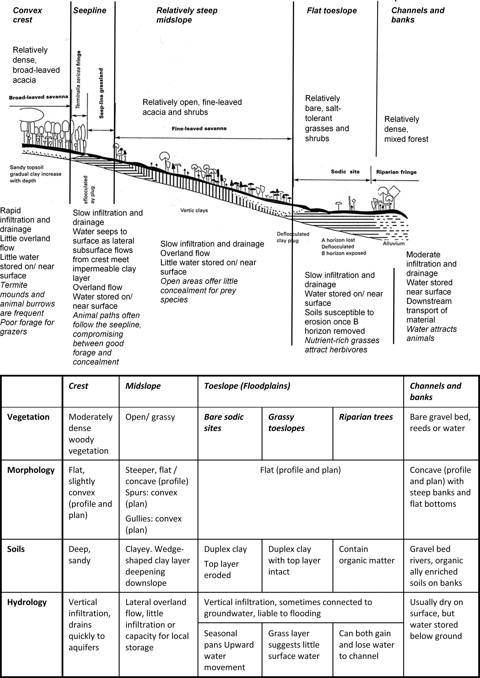
Distinct soil–vegetation associations at various hillslope positions form repeating patterns in the semi-arid, granitic landscapes of southern KNP (Figure 3). These catenal patterns reflect the reciprocal interaction and co-evolution of vegetation, soils and topographically controlled hillslope hydrology (Chappel, 1992; Khomo et al., 2011; Milne, 1935; Venter, 1990). Systematic differences in the biota supported by different parts of these catenas include termite mounds associated with sandy crests (Levick et al., 2010) and sodic sites on the toeslopes, which offer nutritious and plentiful grazing for herbivores (Alard, 2009; Chappel, 1992; Grant and Scholes, 2006; Khomo, 2008).
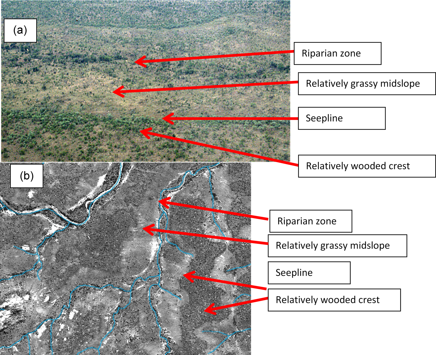
Repeating vegetation patterns in the N’waswitshaka basin. (a) Patterns of woody crests, open grassy midslopes and a wooded riparian strip are repeated on either side of a stream (photograph by Kevin Rogers, October 2004). (b) A SPOT5 pan image (March 2006), with the stream network superimposed, showing the systematic pattern of wooded crests and grassy midslopes. In many places the wooded crests and grassy midslopes are separated by a distinct seepline.
An archetype approach was used to map hillslope units across a 178 km2 (approx. 20 km × 9 km) area of the granitic N’waswitshaka River basin (Figure 4). The basin is finely dissected by ephemeral streams, with an average valley width of 534 m and valley depth of 78 m.
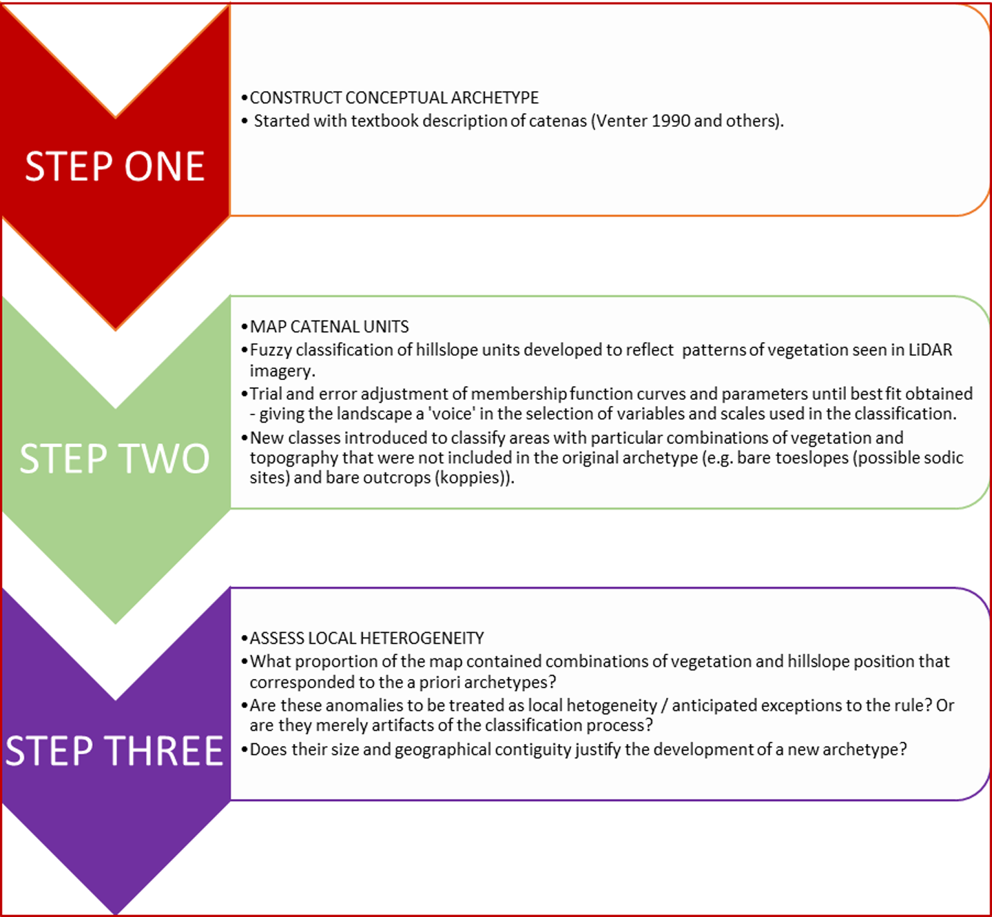
Steps in constructing and representing archetypal landscape units.
1 Step 1: construction of a conceptual archetype
The textbook catena and previous descriptions of the area provided conceptual models that we adopted as an initial set of archetypes to frame our observations of the vegetation patterns of the region (Chappel, 1992; Khomo et al., 2011; Milne, 1935; Venter, 1990) (Figure 5).
A process-based conceptual model of granitic catenas in Kruger National Park (based on Chappel (1992), incorporating work reported, e.g., Chappel, 1992; Gertenbach, 1983; Khomo, 2008; Riddell et al., 2014; Venter, 1990).
These archetypes are underpinned by topographically induced hydrological processes that create and sustain the various soil–vegetation patches associated with each hillslope position. Following short-lived rainfall events, aquifers are recharged via the sandy crest soils, while subsurface macropores transport interflow from the midslopes to the channel (Riddell et al., 2014). As transmission losses from the gravel-bed channels to subsurface aquifers are high, initially intense flows subside quickly, so that low-order channels only flow rarely. Deep bedrock aquifers connect all parts of the landscape. As stream order increases, midslopes tend to become less steep and toeslopes become more prominent as floodplains develop, often containing sodic sites. Soil depth also increases in higher order catchments (Khomo, 2008; Venter, 1990), offering more water storage capacity and increasing both interflow and baseflow.
We based our classification of catenas on easily observable attributes (topography and vegetation) that are known to be related to the contemporary hydrological and ecological processes that sustain the ecosystem and are the focus of conservation management. Different purposes might require different approaches. For example, Sommer and Schlichting (1997) developed a series of archetypes for the classification of catenas in terms of the different ways in which chemical elements have moved between soil pedons to generate the patterns seen today. Such an approach could prove to be useful for understanding patterns of landscape evolution.
Given the interdependence of vegetation, topography, hydrology and soils described in these archetypes, we felt that it was reasonable to represent the a priori archetypal catenal units in terms of topographical and vegetation variables derived from Light Detection and Ranging (LiDAR) data, omitting the less easily observed hydrological and soil domains.
2 Step 2: mapping catenal units
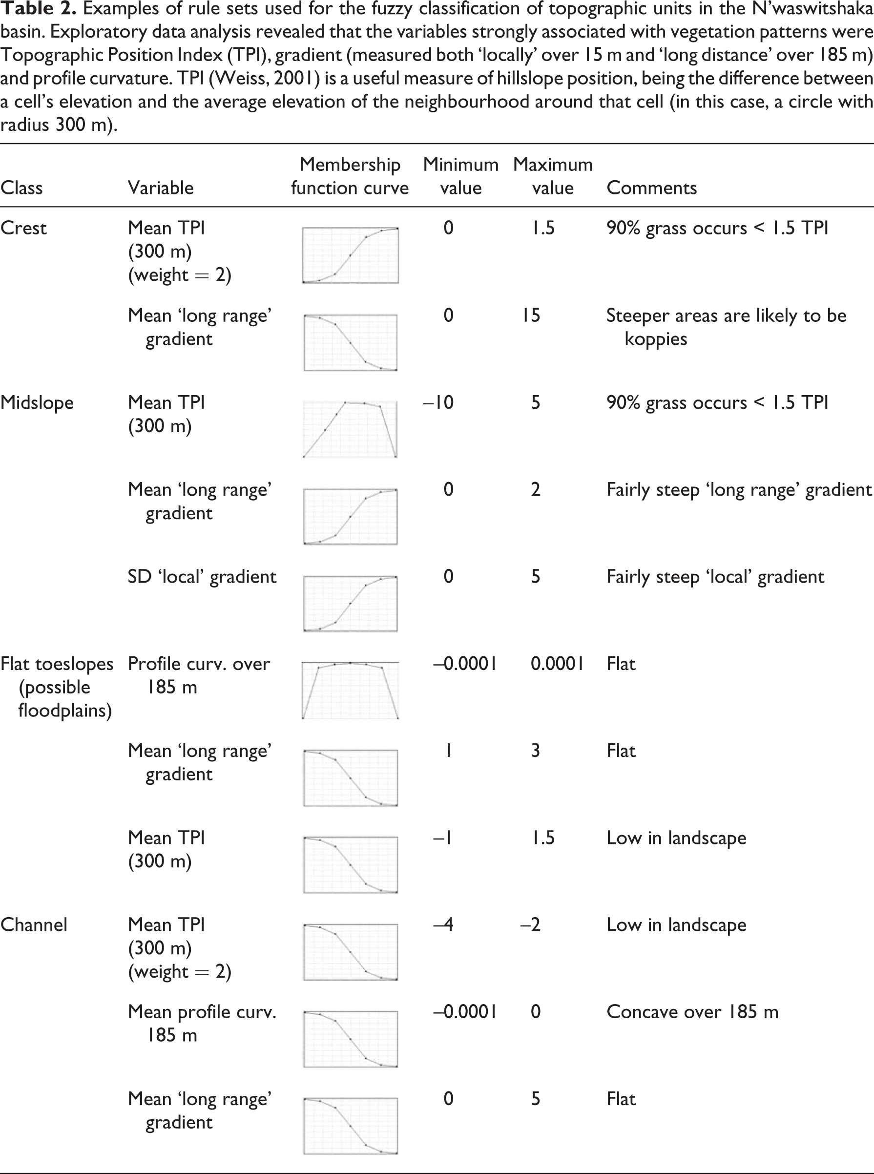
We defined catenal units in terms of intersections between topographical hillslope units (e.g. crests, midslopes, toeslopes and channels) and vegetation patches (e.g. relatively grassy and relatively woody). Topographic units were fuzzily classified using variables derived from LiDAR data that were deemed a priori to be strongly associated with changes in tree canopy cover (Table 2). Both the variables, the scales over which they were defined and the membership function curves for these topographic units were repeatedly refined through an iterative ‘trial and error’ procedure, with the aim of generating topographic units that corresponded to vegetation patterns across the entire study area. For example, ‘crests’ were defined to correspond to elevated areas with relatively woody cover (as seen in Figure 3(b)). Fitting the classification in this way gave the landscape a voice in determining the scales and variables used, echoing the topographic grain (Pike, 1988; Wood and Snell, 1960) and associated vegetation patterns, rather than imposing a standard classification developed elsewhere.
Examples of rule sets used for the fuzzy classification of topographic units in the N’waswitshaka basin. Exploratory data analysis revealed that the variables strongly associated with vegetation patterns were Topographic Position Index (TPI), gradient (measured both ‘locally’ over 15 m and ‘long distance’ over 185 m) and profile curvature. TPI (Weiss, 2001) is a useful measure of hillslope position, being the difference between a cell’s elevation and the average elevation of the neighbourhood around that cell (in this case, a circle with radius 300 m).
Spatial transitions between some classes were quite abrupt, while others were more continuous, with areas of ambiguity reflecting overlap between different classes. For example, image objects classified as ‘crest’ tended to have high membership values, with clear separation from other classes. However, those classified as ‘midslope’ had slightly lower membership values for this class and were somewhat less well separated from a greater number of other classes (Figure 6). (Image objects are clusters of relatively homogenous pixels, defined in eCognition software (Trimble, 1995).)
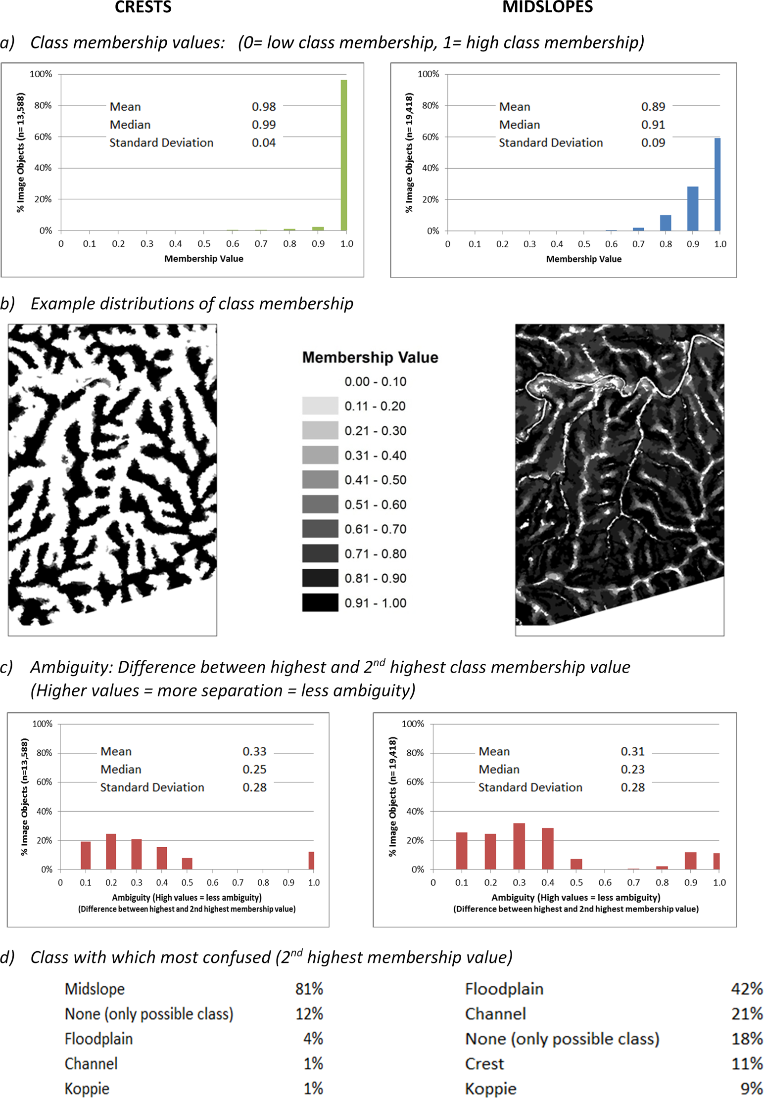
Membership values and ambiguity for crests and midslopes.
Vegetation classification was challenging because it was not easy to separate the generally more dense woody cover on crests from the generally less woody and grassier cover on the midslopes. Thresholds such as Normalized Difference Vegetation Index (NDVI), canopy height and tree density that could potentially separate grass and trees varied considerably over small areas (less than 4 km2), in relation to factors such as species composition, fire history, geology, aspect, etc. We, therefore, developed a classification procedure based on the relative ‘woodiness’ and ‘grassiness’ of neighbouring patches (see Cullum, 2015; Cullum and Rogers, 2011 for details). Since this procedure involved iterative passes over the data, it was not possible to produce a fuzzy classification for relative woodiness and grassiness.
Overlaying the vegetation and hillslope classification data, we refined the definition of hillslope units and vegetation classes to obtain the best possible fit to the a priori archetypes. To achieve this, a categorical classification was produced, assigning image objects to a single class, based on the highest class membership value for each object (Figure 7). Some new classes were defined using combinations of vegetation and topographic data. For example, unvegetated areas on toeslopes were assumed to be ‘potential sodic sites’ and were combined with neighbouring bare areas that formed part of channels, banks or midslopes; likewise, ‘koppies’ (the local name for large rocky outcrops) were defined as steep, unvegetated areas.
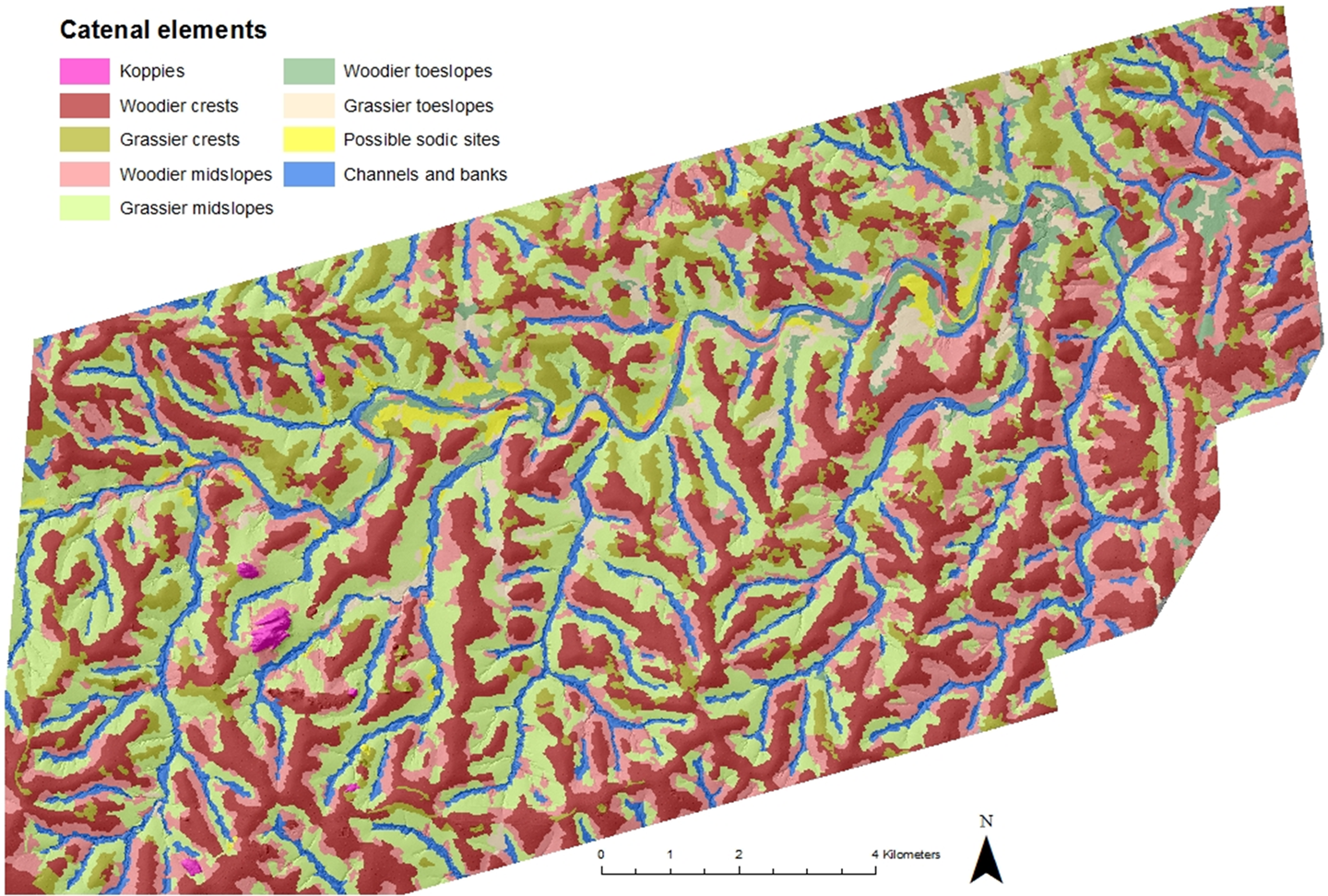
Classification of catenal elements in the N’waswitshaka basin.
3 Step 3: assessment of local heterogeneity
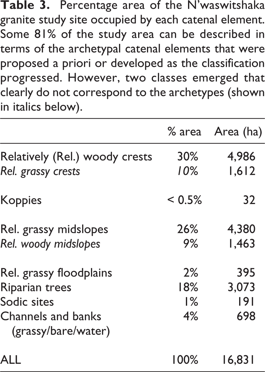
Over 80% of the study site was adequately described by classes corresponding to the a priori archetypes, suggesting that these conceptualisations provide potentially useful descriptions over most of the area. However, despite extensive efforts, the remaining 20% of the study area resisted such classification (Table 3, Figure 8). For example, ‘Relatively grassy crests’ occupy some 10% of the scene, while ‘Relatively woody midslopes’ occupy 9% of the scene and a quarter of all midslopes. These anomalies could be treated as part of the inevitable local heterogeneity and be treated as exceptions to the rule, noting that observations and experience from other sites in archetypal areas cannot be extrapolated to these anomalous areas (as in Notebaert and Piégay, 2013). Alternatively, new archetypes could be developed, accompanied by new or refined conceptual models that link the observed patterns to underlying generative processes. In essence, as these areas are spatially coherent, they could be defined and characterised as genuine classes in their own right.
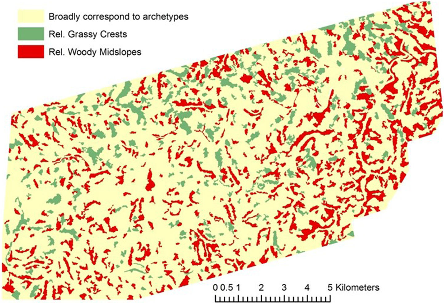
Distribution of areas that do and do not correspond to the a priori archetypes. Areas to the north of the main river and in the west of the scene contain large areas of relatively (Rel.) grassy crests. To the south and east, midslopes are often relatively woody. The idealised conceptual model of woody crests and grassy midslopes applies best in the centre of the scene (see also Figure 6).
Percentage area of the N’waswitshaka granite study site occupied by each catenal element. Some 81% of the study area can be described in terms of the archetypal catenal elements that were proposed a priori or developed as the classification progressed. However, two classes emerged that clearly do not correspond to the archetypes (shown in italics below).
Various issues must be assessed in determining whether or not each of the anomalies challenge the underlying ontology sufficiently to warrant the development of new archetypes or other changes to the classification scheme: Are the anomalies artefacts of the classification, rather than areas where the underlying archetypes and catenal model are unlikely to apply? For example, some areas that have been classified as ‘crest’, due to their high elevation relative to neighbouring areas, are relatively low-lying spurs or mounds towering above the floodplain or river bed. Such areas are perhaps more appropriately classified as ‘midslopes’. Are anomalies situated in transition zones, suggesting that class boundaries need to be refined and/or that the classification (and its representation in a map) needs to be fuzzier? For example, many ‘woody midslopes’ lie above ‘grassy midslopes’, and might be better classified as part of the ‘woody crest’ that lies above. Are anomalies concentrated geographically, suggesting that new archetypes might be needed to better understand and manage a particular area? If so, is this area sufficiently large or important to warrant separate scientific assessment or management? Are the anomalies likely to affect hydrological connectivity, changing flows in ways that are likely to significantly alter the character and behaviour of the subcatchment, deviating from the archetypal model? Are some of the repeated toposequences in this area poorly described by the current archetypes, or is there no visible vegetation difference between crests and midslopes – both are equally grassy or woody?
In the first two instances, refinements to the classification rules could potentially remove the anomalies. However, in the other three instances, hydrological flows are likely to differ from those hypothesised for toposequences of archetypal catenal elements (Figure 5). Identifying these areas as anomalous allows them to be identified either as areas where the archetypal relationships between catenal elements are unlikely to apply, or as areas of ‘grassy crests’ and ‘woody midslopes’ that demand the development of a new archetype (see Figure 7). Analysis of class membership values to assess the similarity of each area to each archetype allows identification of the particular variables responsible for low class membership values (see Figure 6). Such analysis can then inform hypotheses about the reasons for local differences to the archetype.
The vast amount of research conducted in KNP has generated understandings of many different ecological functions and processes in the same system. However, outside long-established and well-used manipulated sites (such as the experimental burn plots and the animal exclosures) it has often proved difficult to integrate findings from these diverse studies due to mismatches in scale or context. In 2012 it was, therefore, decided to establish four research ‘supersites’, which are non-manipulated sites that represent the four major geoclimatic regions of the park: Northern (low rainfall) and Southern (higher rainfall) and basalts and granites. Extensive baseline data and ongoing monitoring will be conducted at these sites, together with ad hoc studies, along the lines of the data-rich long-term ecological research (LTER) sites in the USA, where baseline data, data sharing and a research-enabling environment catalyse data sharing and collaboration between over 1800 scientists (see http://www.lternet.edu). The selection of the sites and the gathering of baseline data have been framed using an archetypal approach, so that future research will also be contextualised within the same perceptions of catenal elements, catchments and physiographic zones (Smit et al., 2013). This approach can also be used to situate sample, reference and motoring sites within the context of the range of variability of the class they represent, recognising that some sites are more representative of the class than others.
VII Discussion and concluding comments
The example from the granitic landscapes of KNP illustrates how archetypes can be used to: mediate between generalised conceptual models (theory) and particular instances (empirical observation); mediate between a landscape and a representation of that reality (i.e. the maps/symbols/language/art we used to describe landscapes); define mappable entities, informing the choice of scales and attributes to delineate landscape units (Cullum et al., 2016); and provide a shared framework for transdisciplinary research and/or facilitate links between policy making, management and science.
Not all landscapes can be (easily) decomposed into a set of structural-functional units that can be clearly and unambiguously delineated and linked to explanatory conceptual models. Indeed, the spatial boundaries of such units are purpose- and scale-dependent and are, therefore, highly uncertain and contestable. Many other sources of uncertainty also exist (see Regan et al., 2002). For example, in tackling ‘causal thickets’, it is difficult, if not impossible, to disentangle interdependent components, process relationships and underlying drivers within explanatory ‘cause-and-effect’ models (e.g. Bowman et al., 2015; Hutchinson, 1948; Wimsatt, 1994). Nevertheless, where agreement can be reached on useful ways to decompose landscapes into process domains, from which units can be mapped, the resulting classification can guide the transfer of learning and experience between locations, structuring a repository of knowledge and providing a rationale for spatial extrapolations and distributed models.
However, such classifications should not be immutable, but must be sufficiently flexible to accommodate local deviations from the general archetype or new or specialised knowledge and experience. No landscape archetype will ever perfectly describe all instances of a given landscape type, so uncertainty will always surround the interpolation of knowledge between different locations (Beven, 1999; Phillips, 2007). However, recognising the extent and type of departures from the archetype and their likely consequences can help to inform assessments of uncertainty and its effects on forecasts and predictions of likely future system behaviour. Recognising and quantifying such anomalies can also provide valuable guidance in the selection of monitoring and sample sites, ensuring that selected sites are those most similar to the class archetype, rather than outliers that are poor representatives of the whole class (e.g. Urban, 2000).
The designation of archetypes and open-ended assessments of landscape diversity have significant implications for environmental monitoring programmes. Not only do they help in determining ‘what to measure’ (Blue and Brierley, 2016; Brierley et al., 2010), but they also provide a way of assessing the degree of heterogeneity (bio-geodiversity) that exists in a given landscape (i.e. quantifying the diversity noted by Blue et al., 2013; Notebaert and Piégay, 2013).
Widespread agreement on a taxonomy of landscape archetypes, while retaining flexibility for local adaptations, would not only facilitate the transfer of learning and experience, but also allow the development of mapping tools and techniques to represent landscapes in terms of these archetypes (see Wheaton et al., 2015). Rapid advances in data gathering and analytical procedures present remarkable opportunities for the monitoring and evaluation of landscape change. In turn, these opportunities highlight the critical importance of the decisions that underpin models and analytical techniques, particularly as those who write the algorithms used to define key landscape attributes, designate their boundaries and assess their change and evolution are increasingly shaping our interpretations of the physical world.
The adaptability of archetypes and their usefulness in appraising the variable degree to which any landscape is described by an archetype prompts increasing attention to consideration of the value of vagueness: As a way of describing real entities that have fluid boundaries. For example, the use of fuzzy classification techniques helps to overcome the challenges of mapping continuous gradients in terms of discrete entities (see also Cushman et al., 2010a; McGarigal and Cushman, 2005). Allowing concepts to have blurred, overlapping meanings means that they can shift to accommodate local realities. Recognising uncertainties in time and space allows imprecision, anomalies and surprises to be embraced rather than avoided. Rather than obscuring local differences by describing patches in terms of averages, ignoring outliers as irrelevant ‘noise’, local heterogeneity can be described in ways that allow users to decide whether or not local differences are important for the purpose in hand.
The outcomes derived from the use of archetypes and fuzzy logic in this study prompt similar lessons to those espoused by Beven and Alcock (2012: 125) in which partial models of ‘everything everywhere’ that are known to be wrong in many aspects form a starting point to test hypotheses and investigate ‘particularities in space’. Much work remains to be done in exposing and debating the archetypes that tacitly underpin such approaches and their management applications (e.g. Lave et al., 2014; Tadaki et al., 2014). In this light, we contend that an archetype approach needs to be tested in a wide variety of landscapes and with diverse groups of designers and end-users.
We challenge cartographers to come up with new ways of representing landscape patterns and connectivity relationships that are more in tune with the underlying conceptualisation of landscapes as dynamic, overlapping patches that are internally heterogeneous and which do not consider all units to be equally similar to the class archetype. Even though spatial classifications based on archetypes are based on a conceptualisation of landscapes that acknowledges landscape complexity, dynamics and the importance of local heterogeneity, the results of such analyses are still shown in terms of area-class maps. This form of representation communicates misleading messages, suggesting that a conventional approach to classification has been used and that boundaries are crisp, classes do not overlap and that landscape units are internally homogeneous. Furthermore, potentially useful information about local heterogeneity is lost. In an alternative approach, raster maps can be used to show membership values for each class separately. However, this form of representation does not ‘objectify’ the classification results. With no distinct landscape units represented, the results are difficult to interpret and use. New forms of representation are also needed to facilitate the conceptualisation and mapping of connectivity and coupling between landscape entities (see Bracken et al., 2013; Okin et al., 2015). Such representations could spur the development of temporal archetypal patterns of landscape flows and responses to change.
The meanings attached to the definition of entities and the mapping of their boundaries may have consequences that extend beyond the initial intentions (or mandated role) of the initial cartographer who designed and produced a map. The range of variability in landscape form is not always cleanly and clearly demarcated into well-defined and meaningful patches and patterns. So, how do we meaningfully design and use maps to communicate variability in the permeability of boundaries and their associated implications for connectivity, giving due regard concerns for variability of process relationships over time?
We have outlined an approach to landscape analysis and mapping that moves away from rigid, standardised classes in which local differences are disregarded, towards flexible approaches that involve the fuzzy definition of both class and positional boundaries and that can be adapted to local circumstances. This approach informs the appropriate scale (grain) to consider landscape units and provides an estimate of how much variation can be expected within a class. The approach provides justification in efforts to put an entity into a class, while also providing more confidence that all elements have been appropriately classified and mapped. Prospectively, this approach can support the development of place-based understandings that build upon emerging technologies in remote sensing and associated analytical techniques to assess where local differences are likely to matter and to hypothesise why and when such differences occur. Importantly, this approach, and resulting applications, draw greater attention to the underlying frameworks that are used to make deliberations in science and environmental management, and the material consequences (and implications for equitable outcomes) that may ensue (see Tadaki et al., 2014). Indeed, explicit expression of underlying conceptual frameworks is a core attribute of recent calls for a more critical physical geography (Blue et al., 2012; Lave et al., 2014).
Footnotes
Acknowledgements
Thanks to Kevin Rogers, University of the Witwatersrand and also to SANParks Scientific Services (especially to Izak Smit, my research coordinator in KNP) for valuable discussions. Thanks are also due to the Andrew Mellon Foundation and the endowment of the Carnegie Institution for Science who facilitated the collection of LiDAR data by the Carnegie Airborne Observatory, from which some of analyses in this paper are derived. Gary Brierley and Carola Cullum acknowledge insights gained from a workshop in Kruger National Park, funded by the South African Water Research Commission. George Perry gratefully acknowledges the support of a University of Tasmania Visiting Scholar fellowship during the writing of this manuscript.
Declaration of Conflicting Interests
The author(s) declared no potential conflicts of interest with respect to the research, authorship, and/or publication of this article.
Funding
The author(s) disclosed receipt of the following financial support for the research, authorship, and/or publication of this article: This research was funded by the South African Water Research Commission (K5/1790) and by a Short Term Doctoral Student Internship Grant from the Faculty of Science, University of the Witwatersrand, Johannesburg. Thanks are also due to the School of Environment at the University of Auckland, who generously hosted the lead author as a visiting scholar.