



Abstract
This article reviews recent scientific progress, relating to four major systems that could exhibit threshold behaviour: ice sheets, the Atlantic meridional overturning circulation (AMOC), tropical forests and ecosystem responses to ocean acidification. The focus is on advances since the Intergovernmental Panel on Climate Change Fifth Assessment Report (IPCC AR5). The most significant developments in each component are identified by synthesizing input from multiple experts from each field. For ice sheets, some degree of irreversible loss (timescales of millennia) of part of the West Antarctic Ice Sheet (WAIS) may have already begun, but the rate and eventual magnitude of this irreversible loss is uncertain. The observed AMOC overturning has decreased from 2004–2014, but it is unclear at this stage whether this is forced or is internal variability. New evidence from experimental and natural droughts has given greater confidence that tropical forests are adversely affected by drought. The ecological and socio-economic impacts of ocean acidification are expected to greatly increase over the range from today’s annual value of around 400, up to 650 ppm CO2 in the atmosphere (reached around 2070 under RCP8.5), with the rapid development of aragonite undersaturation at high latitudes affecting calcifying organisms. Tropical coral reefs are vulnerable to the interaction of ocean acidification and temperature rise, and the rapidity of those changes, with severe losses and risks to survival at 2 °C warming above pre-industrial levels. Across the four systems studied, however, quantitative evidence for a difference in risk between 1.5 and 2 °C warming above pre-industrial levels is limited.
Keywords
I Introduction
Whereas some aspects of climate change can be viewed as becoming proportionately larger with increasing forcings, other aspects may feature more complex, nonlinear behaviour (e.g. Lenton et al., 2008). This can include abrupt and/or irreversible change, which may be associated with key thresholds. Such behaviour must be considered differently in assessments of the potential benefits of mitigation: it implies, for example, that certain impacts could be significantly different above certain levels of anthropogenic interference, although the impacts may not always be negative (Lenton, 2013). Further, thresholds involve systems moving out of the limits of currently observed behaviour, so they require deep process understanding based on a broad range of observations (Kopp et al., 2016). In some cases, early warning of an approaching threshold may be possible (Lenton, 2011).
Clear evidence of threshold behaviour in the Earth system is seen in the paleoclimate record (e.g. McNeall et al., 2011). For example, central Greenland temperatures inferred from ice cores show abrupt changes of 10°C within 100 years (Guillevic et al., 2013) during the last ice age, even though the forcing over this period has evolved smoothly. These changes are thought in part to be associated with changes in the ocean’s thermohaline circulation (Broecker, 2003). Strong paleoclimate evidence also exists for threshold behaviour in major ice sheets and methane reservoirs (McNeall et al., 2011). Various different forms of abrupt shifts have been found in current climate models (Drijfhout et al., 2015), although primarily for different processes than explored in the present review.
This study focuses on four major systems that may feature threshold behaviour: ice sheets, the Atlantic meridional overturning circulation (AMOC), tropical forests and ecosystem responses to ocean acidification. The risk of significant change in these systems is not necessarily linked to large-scale warming alone. Patterns of precipitation can be important for the AMOC and tropical forests; tropical forests are also strongly affected by anthropogenic land use and the direct effect of carbon dioxide, whereas ocean acidification arises directly from increased atmospheric CO2 (although its impacts combine with those of ocean warming) and West Antarctic Ice Sheet (WAIS) stability is influenced by changes in ocean circulation.
The consequences of change in these systems range from amplified global warming through altered climate patterns, elevated sea level and direct loss of biodiversity and ecosystem services (details are given in individual sections in the following). These systems can in principle interact with each other (Lenton et al., 2008), although this is explored in only a few studies.
Here we report primarily on new literature subsequent to that presented in the Intergovernmental Panel on Climate Change (IPCC) Fifth Assessment Report (AR5). As found by O’Neil et al. (2017) in an updated review of IPCC Reasons for Concern, the headline conclusions of AR5 still broadly hold, but there have been considerable advances in understanding. We also briefly consider (in the conclusions) the difference in risk between 1.5 and 2 °C global mean warming above pre-industrial levels. This review was prepared using an iterative approach, by specialists both within and external to the Met Office Hadley Centre. Initial drafts of each section were prepared by the Met Office, then sent to external experts for review and editing (except that for Ocean Acidification, which was prepared by experts in Plymouth Marine Laboratory and the University of East Anglia). The sections were revised accordingly by the Met Office, then sent to the external experts for a second review.
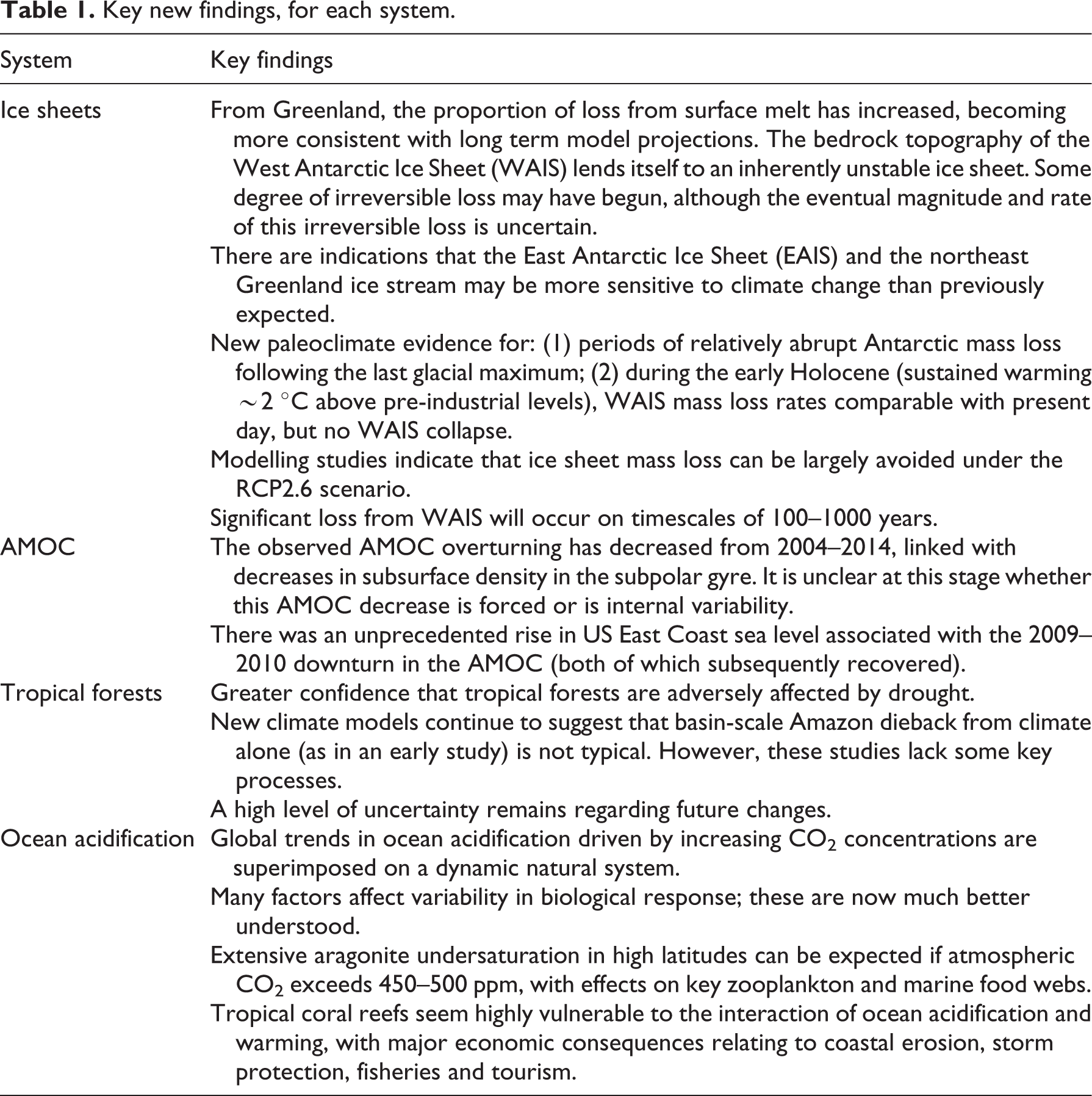
Each system is addressed in a separate section below, each with the following subsections: Introduction (the key issues for that system); Observations (relevant real-world observations); Potential for significant change (literature addressing the question of how likely substantial change is); Consequences (of significant change); Cautions (key scientific uncertainties); and Comparison with AR5. The key conclusions are summarized in Table 1.
Key new findings, for each system.
II Ice sheets
1 Introduction
Ice sheet mass loss, from the Greenland ice sheet (GrIS) and Antarctic ice sheet, is of concern due to its potential impact on global and local sea levels (Alley et al., 2005; Shepherd, 2012), and potential amplification of global warming over long timescales as low-albedo land surface is exposed (Hansen et al., 2008). The ice sheets are the largest potential source of future sea-level rise (SLR) on decadal to millennial timescales. Greenland and Antarctica respectively contain enough ice to raise mean sea level by 7.4 and 58.3 m (Vaughan et al., 2013). In addition, rapid mass loss may have an influence on ocean circulation through a change in salinity and hence density gradients (Yang et al., 2016).
In a state of equilibrium, an ice sheet loses mass (through surface melting, and the calving and submarine melting of its outlet glaciers and ice shelves) (Rignot et al., 2010; Depoorter et al., 2013), at the same rate as it gains mass (through the accumulation of snowfall) (Alley et al., 2005). Increased ice sheet mass loss occurs through two main mechanisms. Increased surface melt is largely driven by higher air temperatures and currently affects Greenland and the Antarctic Peninsula. ‘Dynamic thinning’ (i.e. losses due to increased solid ice discharge into the ocean) involves glacier acceleration and consequent increases in iceberg calving for marine-terminating glaciers and ice shelves, occurring at the fringes of Greenland (Pritchard et al., 2009), the Antarctic Peninsula (Wouters et al., 2015) and West Antarctica (Pritchard et al., 2009; Bingham et al., 2012). This may be induced by increased temperature of the water beneath floating ice or at the glacial terminus (Gille, 2014).
Ice shelves, the floating portions of outlet glaciers, play a key role in modulating the mass balance of the Antarctic ice sheet. They buttress the inland glaciers, controlling the rate of ice leaving the continent and entering the ocean (Dupont and Alley, 2005). Ice shelves are exposed to the underlying ocean and may weaken (Furst et al., 2016) as ocean temperatures rise (Depoorter et al., 2013). If they melt rapidly or break away, ice flow can accelerate, causing net ice sheet mass loss (De Angelis and Skvarca, 2003; Nick et al., 2009) which adds to the rise in sea level. This impact of ice shelf break-up occurred on Larsen-B on the Antarctic Peninsula in 2002, with the consequent acceleration of the glaciers as buttressing was removed (De Rydt et al., 2015). Much of the WAIS is grounded on bedrock below sea level on retrograde slopes (deeper inland). This configuration is inherently unstable and sensitive to small changes at the grounding line (where the ice begins to float) (Mercer, 1968; Schoof, 2007; Durand et al., 2011; Gudmundsson et al., 2012). A small retreat of the grounding line resting on a retrograde slope thickens the ice at the grounding line, in turn increasing the ice flux and inducing further retreat, and so on, until a prograde slope is reached. Hence, local thresholds exist (where the grounding line retreats to a retrograde slope). This is known as the marine ice sheet instability (MISI), and simulations have shown that this is a mechanism for rapid collapse of the WAIS (Gladstone et al., 2012; Cornford et al., 2015; DeConto and Pollard, 2016; Arthern and Williams, 2017).
Iceberg calving has been implicated in the retreat and acceleration of glaciers where ice shelves have disintegrated along the margins of the GrIS and Antarctic ice sheet, indicating that they may be vulnerable to rapid ice loss through catastrophic disintegration (Bassis and Jacobs, 2013). Processes such as fracture propagation in response to local stress imbalances in the immediate vicinity of the glacier front; undercutting of the glacier terminus by melting at or below the waterline; and bending at the junction between grounded and buoyant parts of an ice tongue combine to generate a feedback that accelerates mass loss through increased iceberg calving (Bassis and Walker, 2012). This is known as the marine ice cliff instability (MICI).
Surface meltwater stored in ponds and crevasses can weaken and fracture ice shelves, triggering their rapid disintegration (Scambos et al., 2004). This ice shelf collapse results in an increased flux of ice from adjacent glaciers. This mechanism has been included in one model (Pollard et al., 2015), predicting a SLR from Antarctica of around 1 m by 2100 (Deconto and Pollard, 2016). However, there is uncertainty in this process due to additional effects from surface transport of meltwater onto, across and away from ice shelves. The net result of this transport could either increase or decrease ice shelf stability (Bell et al., 2017; Kingslake et al., 2017).
It is thought that no ice sheet would grow in Greenland if the current one was to be removed, even without human-induced warming, and hence it is a ‘relic’ from the last Glacial Cycle that ended about 12,000 years ago. The altitude of the ice sheet interior maintains the persistently cold temperatures required for the ice sheet to survive. There is a temperature threshold above which the GrIS is no longer viable (Gregory and Huybrechts, 2006; Robinson et al., 2012). This is because, as temperatures increase, so does the area of summer melt, resulting in a lower surface elevation, causing further warming and increased melt (atmospheric temperature decreases with altitude). This positive feedback is known as the small ice cap instability, or melt-elevation feedback (e.g. Crowley and North, 1988; Levermann and Winkelmann, 2016).
Key issues addressed by recent studies include: what the observed ice sheet loss implies for the rate of future global sea-level change, the potential long-term SLR and the possibility of abrupt or irreversible changes on timescales of a few hundred years.
2 Observed recent changes
Between 2002 and 2011, the WAIS contributed 0.3±0.1 mm per year to global SLR (Peng et al., 2016). The majority of this loss has come from basal melt of ice shelves, and associated dynamical thinning, with half the basal melt arising from 10 small ice shelves in the Bellingshausen and Amundsen seas (Rignot et al., 2013). Of these, Pine Island glacier (Favier et al., 2014) and Thwaites glacier (Joughin et al., 2014) are the principal outlets of the WAIS that have rapidly thinned, retreated and accelerated since the 1990s. Recent assessments indicate that Thwaites is contributing ∼0.1 mm per year to SLR, double that of the 1990s, and Pine Island glacier ∼0.13 mm per year; however, there has been no acceleration in mass loss since 2008 (Medley et al., 2014). The spatial pattern of coincident changes in thickness across ice shelves of the Amundsen Sea suggests that the loss of grounded ice is the direct result of increased basal melting of the ice shelf, as a consequence of the inflow of warm water from the Southern Pacific (Jacobs et al., 2011; Ha et al., 2014). Multi-decadal warming at the seabed in the Bellingshausen and Amundsen seas is linked to a shoaling of the mid-depth temperature maximum over the continental slope, allowing warmer, saltier water greater access to the continental shelf in recent years (Schmidtko et al., 2014). Before 2009, the glaciers of the Southern Antarctic Peninsula were in equilibrium, but have since been contributing significantly to SLR at a near-constant rate of 0.16±0.02 mm per year (Wouters et al., 2015). The onset of this sudden and rapid mass loss appears to have a similar origin to that seen in the Amundsen Sea sector. The retrograde bedrock configuration is such that the mass loss is likely to be sustained for years to decades into the future, for this sector of Antarctica.
In addition, there have been synchronous advances and retreats of the calving front of tide-water glaciers of the East Antarctic Ice Sheet (EAIS) (Miles et al., 2013). These appear to be associated with changes in the Southern Annular Mode (SAM), and consequently due to natural climate variability. However, there is evidence of ocean warming causing thinning of the Totten ice shelf, combined with a retreat of the grounding line (Silvano et al., 2016). A substantial area of ice sheet inland of Totten is below sea level, equivalent to 3.5 m of SLR, and consequently the grounding line is potentially unstable due to the MISI. Evidence provided by Silvano et al. (2016) that warm circumpolar water does cross over the EAIS shelf break to cause rapid basal melt for several small ice shelves, suggests that EAIS could be more vulnerable to ocean heat fluxes than previously thought. Overall EAIS currently shows a gain in mass, through increased precipitation, with an implied sea-level fall of 0.32 mm per year over 2009–2011 (Boening et al., 2012).
Estimates of overall sea-level changes associated with net ice loss from Antarctica have been made by the gravity satellite, GRACE, between 2003 and 2014, at 0.25 ± 0.2 mm per year (Harig and Simons, 2015).
The GrIS is losing mass as a result of both increased runoff due to surface melting and increased ice discharge from marine-terminating outlet glaciers (Rignot et al., 2008, 2011; Sasgen et al., 2012; van den Broeke et al., 2009). The Greenland mass loss over the period 2000–2005 contributed about 0.43±0.09 mm per year of SLR. The rate has, however, been accelerating, with estimates for 2009–2012 of 1.05±0.14 mm per year (Enderlin et al., 2014), and for 2011–2014 of 0.74 ± 0.14 mm per year (McMillan et al., 2016). The relative contribution of ice discharge (dynamic thinning) to total loss decreased from 58% before 2005 to 32% between 2009 and 2012. As such, 84% of the increase in mass loss after 2009 was due to increased surface runoff, as opposed to increased discharge (Enderlin et al., 2014). These observations support recent model projections that changes in surface mass balance driven, primarily, by increases in air temperature, rather than ice dynamics, will likely dominate the ice sheet’s contribution to 21st century SLR (e.g. Goelzer et al., 2013; Vizcaino et al., 2015).
The glaciers in the southeast and northwest of Greenland sped up between 2000 and 2005 and have since stabilized or slowed (Enderlin et al., 2014). The slowdown in the southeast has been compensated for by the northeast Greenland ice stream, which extends more than 600 km into the interior of the ice sheet, and is now undergoing sustained dynamic thinning, linked to regional warming, after more than a quarter of a century of stability (Khan et al., 2014). This sector of the GrIS is of particular interest, because the drainage basin area covers 16% of the ice sheet, and numerical model predictions suggest no significant mass loss for this sector, leading to a possible under-estimation of future global SLR (Khan et al., 2014). As for the Southern Antarctic Peninsula, the geometry of the bedrock and monotonic trend in glacier speed-up and mass loss suggests that dynamic loss of grounded ice in this region will continue in the near future (Khan et al., 2014).
3 Potential for significant change
The ice sheets can respond to climate change through accelerated discharge of freshwater to the ocean, and the associated SLR may be irreversible. Accelerated discharge, particularly from a MISI, has implications for the predictability of future SLR. The IPCC AR5 projections of SLR (Church et al., 2013) states that MISI may add tens of centimetres by 2100, but this mechanism was not quantified in the summary projections due to a lack of understanding. New studies here have focussed on the sea-level contribution from the WAIS.
An ice flow model (Gagliardini et al., 2013) revealed that the Pine Island Glacier’s grounding line is probably engaged in an unstable 40 km retreat (Figure 1) (Favier et al., 2014). The associated mass loss increases substantially over the course of the simulations from an average value of 0.05 mm per year observed for the 1992–2011 period, up to and above 0.28 mm per year, equivalent to 3.5–10 mm mean SLR over the next 20 years (Favier et al., 2014). They found that mass loss remains elevated from then on, ranging from 0.16 to 0.33 mm per year. Paleoclimate evidence (Johnson et al., 2014) for the early Holocene (a period of seasonal regional warming about 2 °C above pre-industrial levels) has revealed mass loss from the Pine Island Glacier at a rate comparable to present-day loss, but no collapse. Simulations for the adjacent Thwaites Glacier, also in the Amundsen Sea embayment, indicate future mass losses are moderate (less than 0.25 mm per year) over the 21st century but generally increase thereafter (Joughin et al., 2014). The likely timescale for collapse, based on various imposed ice shelf basal melt rates, is the time required for 100–200 km of grounding line retreat in the Thwaites Glacier system plus 200–1000 years for an actual collapse event (Joughin et al., 2014). Except possibly for the lowest-melt scenario used in the simulations, the results indicate that early stage irreversible collapse has already begun (Joughin et al., 2014). One model includes the process of hydrofracture for Antarctic ice shelves (Pollard et al., 2015; DeConto and Pollard, 2016), associated with surface melt water forcing open crevasses, leading to ice shelf disintegration and MICI. In this idealized simulation, hydrofracture caused a rapid deglaciation of WAIS on a timescale of only about 100 years (from the beginning of major retreat on the Antarctic Peninsula through to peak rate of SLR around year 2140; see their Figure 4c). The ice sheet collapse projected by DeConto and Pollard (2016) does not occur if the strong mitigation scenario of RCP2.6 is followed. Ice loss from the EAIS Wilkes Basin may become substantial over timescales beyond a century (up to 3–4 m SLR after several millennia), with the loss irreversible above a threshold of regional ice loss (Mengel and Levermann, 2014).

Evidence (from Favier et al., 2014) that the Pine Island Glacier’s grounding line is probably engaged in an unstable 40 km retreat, due to the retrograde bedrock slope. Left: Map of bedrock elevation, with the grounding lines for 2009 (white) and 2011 (purple) shown. Right: Bedrock height (solid black line) and geometry of the glacier centreline produced by the Elmer ice flow model at time (t) = 0 (dotted line) and after 50 years of a melting scenario (red line).
Some new understanding of the paleo record has emerged. For Antarctica as a whole, there is evidence (Weber et al., 2014) for periods of relatively abrupt Antarctic mass loss following the Last Glacial Maximum (26,000–19,000 years ago), possibly associated with a positive feedback involving ocean heat transport. It is likely that WAIS collapse occurred in the last interglacial (125,000 years ago), when the Southern Ocean temperature anomaly exceeded 2–3°C (Sutter et al., 2016). However, the solar insolation is sufficiently different in this interglacial, that a similar spatial pattern of warming cannot be achieved through present-day increases in CO2. One study (Levy et al., 2016) combined a range of regional and global paleoproxy information to further constrain the response of Antarctica during the early to mid-Miocene (23 million–14 million years ago), when CO2 levels fluctuated between 280 and 500 ppm (equivalent to pre-industrial levels and a value that will be reached in the next few decades). They identify a peak warming period (16 million years ago) showing a consistent picture of global and regional warming, Antarctic ice sheet retreat, and a corresponding SLR of 10–20 m.
The Southern Ocean as a whole has not warmed significantly over the last decades (Armour et al., 2016). Instead, local warming has occurred, as deeper warm waters have been forced, by increased circumpolar winds, onto the Amundsen Sea continental shelf. Increasing winds are a consequence of global warming, the depletion of stratospheric ozone, or natural variability. Regardless of the cause of the increased windspeed, warm water has reached the continental shelf of the Bellingshausen and Amundsen seas. As a consequence it has been suggested that a critical threshold for grounding line retreat has already been passed for glaciers in the Amundsen Sea sector (Rignot et al., 2014). High ice shelf thinning rates for this and the Bellingshausen Sea sector of West Antarctica over the last two decades (Paolo et al., 2015) combined with the dramatic shift in mass imbalance of the Southern Antarctic Peninsula (Wouters et al., 2015) also point to a widespread shift in behaviour for this region.
It cannot be ruled out that the observed ice shelf thinning is a natural fluctuation rather than a consequence of anthropogenic forcing. Thus, the likelihood of (partial) collapse of the WAIS has not yet been quantified, and requires improved modelling through ice sheet models fully coupled within global atmosphere–ocean climate models. Some progress has been made along these lines, with realistic ice shelf cavities now represented in ocean models (Beckmann et al., 1999; Dinniman et al., 2007; Losch, 2008; Mathiot et al., 2017), and the idealised simulations of MISOMIP (Asay-Davis et al., 2016).
4 Potential consequences
If a collapse of the WAIS were to occur, it would lead to a global SLR of up to 3.3 m (Bamber et al., 2009) on timescales (from the onset of collapse) of 100 years (DeConto and Pollard, 2016) to 400 years (Cornford et al., 2015; Golledge et al., 2015). This inference is supported by records of past SLR. Under the low emissions scenario, RCP2.6, sea-level contributions remain small, and a collapse of WAIS does not occur in simulations (Golledge et al., 2015; DeConto and Pollard, 2016). For Antarctica as a whole, paleoproxy evidence from the Miocene (Levy et al., 2016) suggests potential SLR of the order of 10–20 m, for CO2 levels near 500 ppm.
Surface melt from the GrIS may influence local ocean circulation, through stratification reducing convection in the Labrador Sea (Yang et al., 2016), and consequently local sea-level change, perhaps by 5 cm, in the North-West Atlantic (Swingedouw et al., 2013; Howard et al., 2014).
On centennial to millennial timescales, Antarctic Ice Sheet melt can moderate warming in the Southern Hemisphere, by up to 10ºC regionally, in a 4 × CO2 scenario (Swingedouw et al., 2008). This behaviour stems from the formation of a cold halocline in the Southern Ocean, which limits sea-ice cover retreat under global warming and increases surface albedo, reducing local surface warming. In addition, Antarctic ice sheet melt, by decreasing Antarctic Bottom Water formation, restrains the weakening of the AMOC, which is an effect of the bi-polar oceanic seesaw (Pedro et al., 2011). Consequently, it appears that Antarctic ice sheet melting strongly interacts with climate and ocean circulation globally. It is therefore necessary to account for this coupling in future climate and SLR scenarios.
5 Cautions (uncertainties).
Whereas substantial progress in understanding has been made, it is still unclear what the recent observed changes imply for long-term future ice sheet loss (Wouters et al., 2013), due to regional natural variability. Some observations suggest that there may be a natural cycle of increase and decrease in the rates of mass loss from coastal glaciers (Murray et al., 2010), so short-term trends should not necessarily be extrapolated into the future (Wouters et al., 2013). Indeed, many Greenland glaciers, which accelerated in the early 2000s have since slowed (Moon et al., 2012; Enderlin et al., 2014). There is a possibility that solid earth movement, in response to ice loss, may influence the bedrock slopes, and so reduce further ice loss from the WAIS (Konrad et al., 2015), delaying WAIS collapse by as much as 5000 years.
6 Comparison with AR5
Of the key findings summarized in Table 1, the main new points since AR5 are: observational evidence (Enderlin et al., 2014) that, from Greenland, the proportion of loss from surface melt has increased, becoming more consistent with long-term model projections; evidence that some degree of irreversible loss from the WAIS may have begun (Favier et al., 2014; Joughin et al., 2014; Rignot et al., 2014; Wouters et al., 2015); and indications that the EAIS (Miles et al., 2013) and northeast Greenland (Khan et al., 2014) may be more sensitive to climate change than previously expected.
III AMOC
1 Introduction
The AMOC transports large amounts of heat northwards in the Atlantic Ocean, resulting in a milder climate in northwest Europe and the North Atlantic than would otherwise be experienced (for recent reviews of AMOC behaviour and observations, see Srokosz et al. (2012), Srokosz and Bryden (2015) and Buckley and Marshall (2016)). The IPCC AR5 report (Collins et al., 2013) concludes that it is very likely that the AMOC will weaken over the 21st century, although there is a large spread in the predicted weakening among climate models. A large or rapid (over a decadal timescale) reduction in the AMOC would likely have substantial impacts on global climate, although a collapse (rapid shutdown) of the AMOC by 2100, however, was judged as very unlikely (Collins et al., 2013). These assessments have not changed since the previous IPCC assessment.
2 Observed recent changes
The RAPID-MOCHA array has been observing the AMOC at 26°N since 2004 and now has acquired over a decade of data (Rayner et al., 2011; McCarthy et al., 2015b). This dataset has revealed large variability on timescales from daily to interannual (see Figure 2). This included a large (30%), temporary decrease in AMOC strength over 2009–2010 (McCarthy et al., 2012; Bryden et al., 2014), which resulted in cooling in the upper North Atlantic Ocean in 2010 north of the latitude of the RAPID array and warming to the south (Cunningham et al., 2013; Bryden et al., 2014). This decrease began with a strengthening of the upper mid-ocean recirculation in early 2009 and was compounded by a slowdown in the northward Ekman transport and Gulf Stream flow in late 2009 and early 2010 (accounting for 61%, 27% and 12% of the slowdown, respectively) (Bryden et al., 2014). This decrease was well outside the range predicted for interannual AMOC variability in coupled ocean–atmosphere models (McCarthy et al., 2012; Roberts et al., 2014); note that model resolution may be an issue here. Roberts et al. (2013b) reproduced this AMOC decrease using an initial condition ensemble of ocean simulations driven by observed surface forcing (albeit with too weak an AMOC), suggesting that the atmosphere may have had a dominant role in the temporary AMOC decrease. However, the origin of, and complete explanation for, the 2009–2010 event remains uncertain. To date, no explanations have fully accounted for the changes in Lower North Atlantic Deep Water (LNADW; at 3000 to 5000 m depth) and the lack of change in the Upper North Atlantic Deep Water (UNADW; between 1000 and 3000 m depth) described by McCarthy et al. (2012).

AMOC transport measured at 26.5°N (Smeed et al., 2016). The grey line represents the 10-day filtered measurements, while the red line was produced using a 180-day running mean. Clearly visible are the low AMOC event in 2009–2010 and the overall decrease in strength over the measurement period.
The links between changes in the AMOC, upper ocean heat content and atmospheric response represent an active area of research. For example, the ocean has been implicated in the re-emergence of sea surface temperature anomalies from the winter of 2009–2010 during the following the early winter season of 2010–2011, which contributed to the persistence of the negative winter North Atlantic Oscillation (NAO) and wintry conditions in northern Europe (Taws et al., 2011). Such behaviour may lead to improved predictions of the NAO and winter conditions (Maidens et al., 2013; Scaife et al., 2014).
The AMOC overturning has also decreased from 2004 to 2014 (Figure 2) (Srokosz and Bryden, 2015; Frajka-Williams et al., 2016); the majority of this was due to a weakening of the geostrophic flow (Smeed et al., 2014, who analysed the first eight and a half years of data). This trend has been associated with decreases in subsurface density in the subpolar gyre, similar to those seen in climate models when there is a reduction in the AMOC (Robson et al., 2014). It is unclear at this stage whether the decrease is forced (thus, part of a longer-term downturn). Some recent work suggests that it may be part of a downturn after a previous increase (Jackson et al., 2016; Frajka-Williams, 2015). Statistical tests on the observations (Smeed et al., 2014) suggested that the AMOC decrease is statistically significant, even if the low AMOC event of 2009–2010 is excluded. Roberts et al. (2014) found similar trends as part of natural variability in 2 out of 14 global climate models (GCMs), and in all models considered when corrections are made to include more realistic high-frequency variability. They concluded that more than a decade of observations would be required to detect and attribute an anthropogenic weakening of the same trend as observed over the period 2004–2012 (although this rate does not appear to have been maintained since 2012; see Figure 2). In an earlier model study, Roberts et al. (2013a) estimated that a minimum of two decades of data would be required to detect an anthropogenic trend in the AMOC, based on multimodel 1% per year CO2-forced experiments. This means that the existing AMOC observing system would need to make measurements until at least 2024. Another study (Mercier et al., 2015) analysed repeat hydrographic data along a Greenland to Portugal section from 1993 to 2010, finding an overall decline in the AMOC over that period. Send et al. (2011) observed a decreasing trend in the transport of the deep western boundary current at 16oN (one component of the AMOC) over a similar period. In the South Atlantic, based on a combination of satellite altimeter and hydrographic observations, Dong et al. (2015) noted that ‘since 2010 the MOC has exhibited low values when compared to the 1993–2011 mean values’. Linking the observations of the AMOC obtained at different latitudes by different observational means remains a significant challenge (Elipot et al., 2014, 2017). Landerer et al. (2015) showed that satellite observations of ocean bottom pressure may provide a useful method for examining latitudinal coherence of signals, however it is currently restricted to detrended data and regions of steep topography.
A recent paper (Rahmstorf et al., 2015) suggested that the trend detected at 26°N is part of an ‘exceptional slowdown’ of the AMOC. They found a relationship between sea surface temperatures and the AMOC in a climate model and then use reconstructions of surface temperatures from paleoclimate records to suggest that there has been a weakening that is unprecedented over the last 1000 years. There are, however, inherent uncertainties around both the relationship used and the temperature reconstructions, raising questions over whether the results are robust. In contrast, a recent reconstruction of the AMOC in the South Atlantic since 1870 (Lopez et al., 2017) suggests that it is presently in a stronger than normal phase. Ultimately, all proxies for the AMOC, such as temperature, coastal sea level (Ezer, 2015; McCarthy et al., 2015b; Frajka-Williams, 2015) or gravity measurements (Landerer et al., 2015) need to be tested and verified against direct observations of AMOC strength, over the timescales of interest, if they are to be used to infer robustly its behaviour over longer periods.
Future observations and research will improve our assessments of past and on-going AMOC changes. In this context note that the Overturning in the Subpolar North Atlantic Program (OSNAP) (Lozier et al., 2017) deployed instruments in 2014 along a line from Canada to Greenland to Scotland, to observe the AMOC in the subpolar gyre, complementing the 26.5°N observations in the subtropical gyre. Meanwhile, in the South Atlantic there are trans-basin observations of the AMOC beginning to be made at 34.5°S (SAMBA: South Atlantic MOC Basin-wide Array) (Meinen et al., 2013; Ansorge et al., 2014). Recently, a new component of the AMOC, the so-called East Greenland spill jet, has been identified from a year of mooring observations (von Appen et al., 2014), but its importance in the long term for the overall AMOC remains to be confirmed.
3 Potential for significant change
Paleoclimate studies have suggested that some abrupt changes to climate may have been caused by the AMOC switching from an ‘on’ state, where it transports heat northwards in the Atlantic, to an ‘off’ state (Rahmstorf, 2002). Paleoceanographic studies of the AMOC and abrupt climate change over the last glacial cycle have been recently summarized by Lynch-Stieglitz (2017), who found that the evidence for changes in the AMOC associated with the Younger Dryas and many Heinrich events is strong, and there is some evidence for AMOC changes over many Dansgard-Oeschger events. However, the ultimate causal links between the co-incident changes in the AMOC and climate are less clear. Further, these studies are hard to interpret in terms of future change, as the conditions in which past abrupt changes occurred were very different to the present. It is thought that abrupt changes may be related to the existence of bistability (where both ‘on’ and ‘off’ states of the AMOC can exist for a given forcing) as predicted by theoretical models of the Atlantic (e.g. Stommel, 1961), Earth system models of intermediate complexity (Rahmstorf et al., 2005) and studies with low-resolution global circulation models (Hawkins et al., 2011; Manabe and Stouffer, 1988). Statistical properties of the timeseries of AMOC strength may give warning of approaching a threshold, however a new model study finds that centuries of data from a reliable proxy would be required (Boulton et al., 2014).
There have been many model studies suggesting that the stability of the AMOC might be affected, or even controlled, by whether the AMOC imports or exports freshwater from the Atlantic, because this can indicate the presence of a positive or negative advective feedback. de Vries and Weber (2005) found that the freshwater transport by the AMOC into the Atlantic was an important indicator of stability in their experiments. The relative importance, for AMOC stability, of freshwater export/import by the AMOC itself, is unclear, however. Other factors have subsequently been found to be important in determining AMOC stability. For example, Jackson (2013) found that, whereas the overturning component of freshwater transport does partially indicate the sign of the advective feedback in a GCM, the transport of freshwater by the gyres can also play a crucial role. Swingedouw et al. (2013) also found that gyre transports can affect the magnitude of AMOC reduction. The presence of eddies is lacking in many models (due to low resolution) but studies with an eddy resolving model show that they can also affect the freshwater transport (den Toom et al., 2014). Mecking et al. (2016) found that the AMOC in an eddy-permitting model was very slow to recover from an input of freshwater. They found that the freshwater transport by the AMOC was important for maintaining the weak AMOC state, and hypothesised that this transport was changed by the eddy-permitting resolution. Understanding these controls on AMOC stability is crucial to constraining the likelihood of AMOC collapse. A recent paper (Liu et al., 2017) has noted that biases in the models may affect the estimated probability of an AMOC collapse.
4 Potential consequences
A collapse in the AMOC would cause a large relative cooling over the North Atlantic, which would have wide-ranging impacts, such as cooling in the northern hemisphere, warming in the southern hemisphere, and a southward shift in the Inter Tropical Convergence Zone, causing substantial changes in tropical precipitation (Vellinga and Wood, 2008; Jackson et al., 2015).
The Amazon is one region sensitive to change in the AMOC, but the impacts are uncertain. A recent study by Parsons et al. (2014) found that a reduction in the AMOC caused an increase in vegetation over the Amazon, due to a change in precipitation seasonality (despite a reduction in annual mean precipitation). This contrasts with an earlier study (Bozbiyik et al., 2011), which found that a reduction in the AMOC causes large reductions in Amazon vegetation due to precipitation reductions.
Other studies have concentrated on impacts over Europe. Jackson et al. (2015) confirmed an earlier study by Woollings et al. (2012), that a reduction in AMOC strength could drive an increase in the number of winter storms across Europe. Jackson et al. (2015) also showed that the increase in winter storms resulted in greater precipitation over western coasts in Northern Europe, despite a general reduction of precipitation over the northern hemisphere from a cooling-induced reduction in evaporation. They also found regional changes in summer precipitation across Europe, similar to those associated with Atlantic sea temperature found by Sutton and Dong (2012). Haarsma et al. (2015) examined the relationship between European atmospheric circulation and the AMOC across the CMIP5 ensemble. They also found an influence of AMOC strength on European summer precipitation and cloud cover.
One impact of the AMOC suggested recently is its possible role in the so-called global warming ‘hiatus’ (Chen and Tung, 2014), though various other explanations for the hiatus have been proposed. Another recently observed impact is the reduction in uptake of CO2 by the Atlantic Ocean due to the weakening of the AMOC over the period 1990 to 2006 (Perez et al., 2013).
Another recent focus of attention has been the role of the AMOC in SLR on the eastern seaboard of the USA (Ezer, 2015; Goddard et al., 2015; McCarthy et al., 2015a; Yin et al., 2009). In particular, Goddard et al. (2015) demonstrated that the 2009–2010 temporary downturn in the AMOC led to an unprecedented 12.8 cm SLR along the coast north of New York over the same period. They show that this rise was a 1-in-850-year event. Furthermore, they note that, ‘Unlike storm surge, this event caused persistent and widespread coastal flooding even without apparent weather processes. In terms of beach erosion, the impact of the 2009–2010 SLR event is almost as significant as some hurricane events’. This observed short-term change provides evidence for what has been previously suggested only by modelling studies (Levermann et al., 2005), that a slowdown or collapse of the AMOC would lead to significant SLR on the eastern seaboard of the USA.
5 Cautions
There are large inter-model differences in projections of future AMOC decline amongst models used for the IPCC AR5 report. Reintges et al. (2016) found that uncertainties in AMOC projections were dominated by uncertainties in freshwater changes amongst the models, with contributions from uncertainties in both changes in surface freshwater fluxes and ocean freshwater transports.
Several studies have shown that many GCMs have biases in the freshwater transport of the AMOC (importing instead of exporting freshwater), and that this might affect the simulated stability of the AMOC. The source of this bias is unclear. Jackson (2013) attributed the bias to an over-evaporative Atlantic in the model and notes the difference from observations in salinity profiles in the South Atlantic. Liu et al. (2014) suggested that the presence of a double Atlantic Inter Tropical Convergence Zone (a common GCM bias) results in a tropical salinity bias that stabilizes the AMOC. Another source of uncertainty is the transport of saline water from the Indian Ocean to the Atlantic by eddies that are shed from the Agulhas current. Current GCMs do not resolve the scales required to correctly represent these eddies, but a recent study by Biastoch and Böning (2013) used a high-resolution nested model to resolve this region. They found that a southwards shift of the southern hemisphere westerlies (as is expected to occur under anthropogenic climate change) results in a decrease in salinity transport into the Atlantic, however this change in salinity is small and has little impact on the AMOC. The lack of eddy-resolving resolutions in current GCMs might also have an impact on the transient response of the AMOC to increased freshwater input (Weijer et al., 2012; Mecking et al., 2016).
There is also substantial uncertainty about the future inputs of freshwater into the Atlantic, particularly since the climate models lack dynamic ice sheet models that could substantially speed up the input of freshwater from the GrIS. Separate studies including additional freshwater inputs from the GrIS find that projected changes do not have major impacts on the AMOC, although there is uncertainty about future changes in freshwater fluxes from Greenland (Bamber et al., 2012). Böning et al. (2016) concluded that meltwater from the GrIS has resulted in a gradual freshening of Labrador Sea, but that this has had no significant impact on the AMOC yet. A recent study found that the MOC became less sensitive to freshwater inputs when CO2 levels were high, because of increases in stratification caused by warming and changes in the wind-driven circulation (Swingedouw et al., 2015). Another study suggests that future increases in precipitation over the Arctic, leading to increased freshwater flux into the North Atlantic could also affect the AMOC (Bintanja and Selten, 2014). The most recent GCM study that accounted for Greenland melting (Bakker et al., 2016) concluded that GrIS ‘melting affects AMOC projections, even though it is of secondary importance’.
6 Comparison with AR5
The main development since the publication of AR5 has been the updated observations of overturning from the RAPID-MOCHA array (Smeed et al., 2014; Srokosz and Bryden, 2015), which shows a decline over the period 2004–2014. Studies suggest that this was related to decadal variability. This does not preclude the presence of a longer-term decline, but the time series is too short to make definitive statements. Continuous observations from the existing AMOC observing system until at least around 2024, combined with further understanding of the past record from multiple proxy information, and more model studies, will be required to isolate a forced decline in the AMOC. Another key finding is the unprecedented rise in US east coast sea level associated with the 2009-10 downturn in the AMOC (both of which subsequently recovered). Although this is a change on a shorter timescale than the 100-year timescale associated with climate change, it shows that changes in the AMOC may have impacts on multiple timescales. Finally, the inclusion of Greenland melting in GCMs has been found to affect AMOC projections, but appears to be of secondary importance.
IV Tropical forests (Amazon focus)
1 Introduction
Tropical forests regulate and supply to society a range of services, which bring benefits at global to local scales. As well as sustaining high biodiversity they influence climate through biogeochemical (carbon cycle) and biophysical (water and energy) mechanisms. Over the period 1990–2007, intact tropical forests took up carbon at the rate of 1.2 ± 0.4 Pg C per year (corresponding to about half the global land carbon sink), compared with 0.50 ± 0.08 Pg C per year by the boreal forests (Pan et al., 2011), and around 1.1 ± 0.8 Pg C per year losses of forest carbon stocks to the atmosphere through land use change over 2000–2009 (Settele et al., 2014). However, large droughts can cause elevated mortality rates, especially for larger trees (Phillips et al., 2010; Nepstad et al., 2007; da Costa et al., 2010; McDowell and Allen, 2015) and temporary shifts from ecosystem carbon sink to carbon source (Phillips et al., 2010; Lewis et al., 2011; Gatti et al., 2014). Estimates of the impact of the 2005 and 2010 Amazon droughts (mostly through increases in tree mortality during and lagging the droughts) stand at 1.6 and 2.2 Pg C, respectively (Phillips et al., 2009; Lewis et al., 2011).
Tropical forests are subject to interacting effects from atmospheric CO2, climate and land-use change (e.g. Coe et al., 2013). Land-use change effects include direct deforestation, and accidental ‘leakage’ fires (where intentional fires spread accidentally over a wider forest area). Forest fragmentation (an important by-product of deforestation) lengthens the forest edge. Since most forest fires occur at the forest edge, because of greater human activity, fragmentation accelerates the rate of forest erosion by fire. Deforestation increases albedo and reduces evapotranspiration, altering climate both locally and downwind; aerosols from deforestation fires may also reduce rainfall (Marengo et al., 2011). Climate change could alter vegetation productivity and mortality, both directly and indirectly by modifying fire behaviour. Increased atmospheric CO2 may increase tree growth (where nutrients are not limiting), but also increase tree mortality from lianas (vines). The full vegetation response to CO2 and climate changes may take decades to be completely realized (Jones et al., 2009), and the subsequent carbon release even longer.
The AR5 finds that large-scale dieback due to climate change alone is unlikely by the end of this century (medium confidence). However, it states with medium confidence that ‘severe drought episodes, land use, and fire interact synergistically to drive the transition of mature Amazon forests to low-biomass, low-statured fire-adapted woody vegetation’ (Settele et al., 2014). New research has largely, but not exclusively, focused on the Amazon: due in part to early climate model projections of climate-driven Amazon dieback (Cox et al., 2000). Severe Amazonian droughts in the last decade have provided insights on forest responses to extreme dry conditions. In addition to forest and climate monitoring, throughfall exclusion and prescribed-burn experiments have allowed in-situ study of the effects of longer-term drought and fire. Numerical studies have also increased in number and progress has been made in putting the early results into context.
2 Observations
New studies have given greater confidence that the Amazon represents a long-term net carbon sink (Brienen et al., 2015; Espirito-Santo et al., 2015; Gatti et al., 2014), but also suggest (Brienen et al., 2015) that its strength has weakened progressively as tree mortality rates increase (Figure 3). Potential drivers for the mortality increase include more frequent or more severe droughts, and feedbacks of faster growth on mortality, resulting in shortened tree longevity (Bugmann and Bigler, 2011).

Trends in net above-ground biomass change, productivity and mortality rates, for 321 plots, weighted by plot size (after Brienen et al., 2015).
The response of trees to elevated CO2 remains uncertain. Some recent longer-term studies of tropical tree rings (van der Sleen et al., 2015; Battipaglia et al., 2015; Groenendijk et al., 2015) have found no evidence for sustained increases in tree growth or carbon uptake, but as Brienen et al. (2012) pointed out, tree-ring studies are subject to biases that preclude robust statements about ecosystem-level changes. So far, multi-decadal plot data have been used systematically to probe recent growth trends at continental scale only in Amazonia (Brienen et al., 2015). Here they indicate a long-term increase in growth rates since the 1980s, as well as a lagging increase in mortality rates, consistent with a long-term growth stimulation, such as by CO2.
There is greater confidence that Amazon forests are adversely affected by drought. There has been new work on the response to the 2010 drought, and also the 1997 and 2005 events (Tomasella et al., 2013). A new attribution study (Shiogama et al., 2013) of the 2010 drought showed that, whereas sea surface temperature anomalies in the tropical Pacific and Atlantic likely increased the probability of drought (in addition to biomass burning) (Marengo et al., 2011), unforced atmospheric variability probably also played a large role. Atmospheric measurements (Gatti et al., 2014) confirmed earlier plot-based findings (Phillips et al., 2010; Lewis et al., 2011) that the Amazon switched from a temporarily from a net carbon sink to a source during the 2010 drought. Compared with these short-term natural droughts, the impact was seen to be much stronger in the long-term persistent experimental droughts induced by a forest throughfall exclusion experiment in eastern Amazonia (da Costa et al., 2014), and by 2014, 13 years of 50% throughfall exclusion at Caxiuana had caused a cumulative biomass loss of 45.0 ± 2.7% (Rowland et al., 2015). Consistent with previous suggestions that effects of a single drought persist for several years (Saatchi et al., 2013; Phillips et al., 2010), even during the anomalously wet year of 2011, the Amazon was still estimated to be carbon neutral overall (Gatti et al. 2014), possibly due to lagged effects of the 2010 drought.
Drought mortality, especially in larger trees, is a major pathway for carbon release (Phillips et al., 2010; Nepstad et al., 2007; da Costa et al., 2010), but underlying mechanisms are not well understood (Meir et al., 2015), and poorly represented in current vegetation models (Powell et al., 2013). However, hydraulic failure is suggested as the primary cause from the Caxiuana drought experiment (Rowland et al., 2015). A study of detailed plot-level responses to the 2010 drought in several sites, compared with other years (Doughty et al., 2015) suggested that trees may prioritise growth in response to reduced photosynthesis from short-term drought, leaving some trees more vulnerable to mortality. In contrast, the long-term (>12 years) response to persistent experimental rainfall exclusion (Rowland et al., 2015), shows no decline in photosynthetic capacity (although photosynthesis may have declined if mean stomatal conductance declined), but an increase in leaf dark respiration in tree taxa vulnerable to drought mortality (possibly a sign of drought stress). It has been suggested that early warning of drought mortality events may be plausible based on observations of tree properties (Camarero et al., 2015). Overall, the AR5 viewpoint of persistent drought causing a shift towards lower statured, low-biomass forest is retained (Rowland et al., 2015).
Drought can also cause abrupt increases in fire-induced tree mortality over sub-seasonal timescales (Brando et al., 2014), driving a lagged increase in carbon emissions over subsequent years. More than 85,500 km2 of the southern Amazon was burnt by understorey fires during 1999–2010, with evidence for a strong climate control on fire (Morton et al., 2013).
Forest responses to warming remain uncertain, and more forest warming field experiments are needed (Cavaleri et al., 2015). In one such experiment (Slot et al., 2014), although respiration increased with warming, thermal acclimation did occur. A new meta-study integrating experimental and observational results (Vanderwel et al., 2015) suggests that acclimation could potentially half increases in leaf dark respiration over the century, compared with null model expectations that ignore acclimation. On the other hand, a global-scale analysis of interannual variability has suggested (Anderegg et al., 2015) that nighttime respiration in tropical forests may be highly sensitive to warming.
Some new observational studies have found substantial reductions in evapotranspiration in some (Oliveira et al., 2014; da Silva et al., 2015; Panday et al., 2015), but not all (Rodriguez et al., 2010) deforested regions. The full effects of deforestation over the Xingu river basin (a southeast tributary of the Amazon) may have been masked by climate variability (Panday et al., 2015).
3 Potential for significant change
A recent review of wider sources of evidence (Coe et al., 2013) identified South/South-East Amazonia as particularly vulnerable: due to high deforestation rates locally and in the upwind savanna region; its susceptibility to small climate shifts (being in a transitional climate zone between forest and savanna); and greater climate model agreement on future rainfall reductions in this region (compared with the West Amazon). A review for African rainforests (Malhi et al., 2013) highlighted similar points: whereas deforestation rates have historically been relatively low over Africa, there is potential for significant future increases; and African forests have climate close to the limit of rainforest sustainability. Models tend to predict rainfall reductions (increases) over western (central) equatorial Africa (James et al., 2014). Rainfall decreases over west equatorial Africa can be large in some models (James et al., 2014), although the forest response is hard to predict.
The observations and field experiments summarized above have given greater confidence that forests are significantly affected by drought, emphasising the importance of extreme climate events in causing extensive tree losses (through drought and heat mortality and increased fire). On the other hand, some acclimation of trees to warming has been demonstrated. These vegetation responses are not well understood or represented in current dynamic vegetation models (e.g. Powell et al., 2013).
A recent study using three terrestrial biosphere models (Zhang et al., 2015) found the direction and severity of precipitation change to be critical. A greater model consensus for a projected lengthening and deepening of the dry season in Amazonia was found in CMIP5 compared with CMIP3 (Joetzjer et al., 2013), although it is unclear whether this represents a statistically significant improvement in model performance. A new observationally constrained model study (Boisier et al., 2015) found a greater lengthening of dry seasons over the Amazon than projected by unconstrained models (as found, with a different method, by Shiogama et al. (2011)). A key uncertainty in terms of impacts is the extent to which forest whole-ecosystem responses to climate change might be protected by the wide functional diversity in many tropical forests. The work of Fauset et al. (2012) from Ghana suggests that by not accounting for biological diversity, most vegetation models may underestimate forest resilience.
In terms of land use, it has become clearer that as well as direct deforestation, the indirect effects of deforestation on forest fragmentation, and on climate locally and downwind, must be considered in regulatory policies (e.g. Harper et al., 2014; Lawrence and Vandecar, 2015; Brinck et al., 2017; Wu et al., 2017). Whereas a 70% decline has been reported in deforestation in the Brazilian Amazon between 2005 and 2013 (Nepstad et al., 2014), maintaining low levels of deforestation in a sustainable manner remains a challenge (Nepstad et al., 2014). Despite the reduction in deforestation since 2004, around half of the area burnt during 1999–2010 over the southern Amazon occurred during 2007 and 2010, when deforestation activity was relatively low, suggesting that fire-free land use needs to be encouraged as well as reducing direct deforestation (Morton et al., 2013). Achieving similar reductions in deforestation in other countries may be challenging due to issues with governance and monitoring capability (DeFries et al., 2013), but for Indonesia, accounting for spatial variation in costs and benefits of avoided deforestation does reveal low-cost options (Graham et al., 2017).
Various positive feedbacks (fire–vegetation and climate–vegetation; see e.g. Hirota et al. (2011), Staver et al. (2011) and Hoffmann et al. (2012)) exist that could lead to abrupt reductions in forest cover, for relatively small change in external forcings, and inhibit reversibility, but the processes are poorly characterized. The timescale of any abrupt change depends on the processes and the spatial scale considered, and may be strongly dependent on stochastic climate variability. Very locally, loss of tree cover from fire or drought mortality can occur over seasonal timescales in the event of severe drought. However, one model study (Higgins and Scheiter, 2012) found that, while transitions between vegetation states may be abrupt locally, over continental and larger scales the effect on the carbon cycle is much more gradual (because the timing of transitions varies with location). It has been suggested (Verbesselt et al., 2016) that temporal autocorrelation in satellite data provides evidence for threshold behaviour in forests, and potential for monitoring forest resilience. Evidence for alternative stable states has recently been reported in vegetation height (Xu et al., 2016) as well as in tree fractional cover (Staver et al., 2011; Pausas and Dantas, 2017; Hirota et al., 2011). However, the spatial scale over which abrupt or irreversible change might extend depends on the strength of these positive feedbacks compared with environmental control on vegetation cover, and demonstrating whether alternative stable states exist over large scales is challenging (Good et al., 2016; Staal et al., 2016). Spatial interaction between forest and savanna can reduce the area over which alternative stable states exist (a clear exploration is provided by Staal et al. (2016)). Indeed, recent observational work has challenged the notion that savanna and forest represent ‘alternative stable states’ over large areas of the tropics (Veenendaal et al., 2015; Wuyts et al., 2017). Local fire–vegetation feedbacks are seen in prescribed burning experiments (Silverio et al., 2013), but, over large scales, only 10% of the locations burnt in the 2005 drought showed repeated burning by 2010 (Morton et al., 2013). A model study (Moncrieff et al., 2014) found that the area over which alternative stable states are possible could be large in present-day conditions, but declined substantially with future CO2 increases. Hoffmann et al. (2012) noted that forest–fire feedbacks themselves can be sensitive to tree growth-rates and, hence, to climate change.
4 Potential consequences
The observations summarised above give greater confidence that the Amazon represents a net carbon sink, but this appears to have been declining at least for a decade, and the long-term future of this sink is uncertain. Persistent drought would be likely to cause a transition to lower statured, lower biomass forest, from mortality of larger trees (Rowland et al., 2015), and severely threaten biodiversity (Esquivel-Muelbert et al., 2017). Extreme events over the Amazon could have a large impact on the global carbon cycle and offset or counteract potential regional increases in biomass (Reichstein et al., 2013).
Whereas it is accepted that tropical deforestation tends to reduce evapotranspiration locally, consequent changes in rainfall are complex and depend on the scale and pattern of deforestation (Lawrence and Vandecar, 2015). Including deforestation feedback on climate (via precipitation) is key in assessing river runoff change (Stickler et al., 2013; Lima et al., 2014). Stickler et al. (2013) estimated that when feedbacks on climate are included, the sign of change in hydropower generation potential for the plants under construction on the Amazonian Xingu River is reversed, declining to 25% of maximum plant output by 2050 under business-as-usual land-use projections (with 40% deforestation by 2050). The net runoff response in the Amazon is basin-dependent (Lima et al., 2014) and is sensitive to the scale and pattern of deforestation (Lawrence and Vandecar, 2015). Deforestation may reduce the length of the wet season, such that large-scale expansion of agriculture in Amazonia may be unsustainable (Oliveira et al., 2013; Arvor et al., 2014). Land-use-driven stream warming of at least 3–4 °C (in mean daily maximum temperature) in Southeastern Amazonia has also been observed (Macedo et al., 2013), well above the ∼1 °C threshold for changes in fish physiology, growth and behaviour. Overall, multiple ecosystem services need to be taken into account when considering optimal management (Donoso et al., 2014).
5 Cautions (uncertainties)
Accurate projections are partly limited by the availability of observations. Inaccessibility of tropical forests increases reliance on remote sensing data, but also makes verifying remote sensing data (notably, precipitation, biomass and vegetation productivity data) challenging. New studies have shown that great caution is required in interpreting satellite retrievals of variability in greenness (Morton et al., 2014). The tropical forest biome constitutes one of the largest terrestrial carbon sinks, but it is also associated with relatively large uncertainties (Pan et al., 2011), because of its great ecological complexity, huge scale and multiple anthropogenic processes affecting it (Lewis et al., 2015).
There is substantial uncertainty in the CMIP5 projections of future precipitation in tropical forest regions (Collins et al., 2013), although there is greater degree of inter-model agreement in some seasonal changes, such as a lengthening and a deepening of the dry season in Amazonia (Joetzjer et al., 2013; Boisier et al., 2015). However, the representation of present-day Amazon precipitation still contains large biases. Large uncertainties are also associated with the modelled response of vegetation to temperature (Galbraith et al., 2010; Huntingford et al., 2013) and to CO2 (Rammig et al., 2010). Processes of direct mortality from fire and drought (and effects of fire on aerosol) are often either unrealistic or absent from models (e.g. Powell et al., 2013), and the range of plant functional types is extremely limited in relation to the large biodiversity and, hence, range of potential tree-level responses in most tropical forests.
6 Comparison with AR5
The new literature has not altered the broad, general view given in AR5. Probably the greatest advances lie in increased confidence that, at least over the Amazon, drought adversely affects the forest carbon balance and improved understanding of how this occurs. Many uncertainties remain, and estimating the likelihood of basin-scale forest dieback remains challenging.
V Responses to ocean acidification
1 Introduction
Increased concentrations of atmospheric CO2 reduce seawater pH, increase the solubility of calcium carbonate (reducing saturation state) and cause other chemical changes, together known as ocean acidification. The biogeochemical, ecological and societal implications of ocean acidification have received greatly increased research attention during the past decade (Riebesell and Gattuso, 2015; Mathis et al., 2015). Ocean acidification risks and impacts were included as a component of climate change in the IPCC’s Fourth Assessment Report, with more detailed analyses in the AR5, particularly by Working Group II (Portner et al., 2014).
Analyses of geological ocean acidification events and modelling studies show that physico-chemical recovery from perturbations in ocean carbonate chemistry of similar magnitude to projected changes takes many thousands of years (Zeebe and Ridgwell, 2011), due to slow rates of deep ocean mixing and of chemical equilibration with seafloor sediments. The rate of CO2 increase today is estimated to be around 10 times faster than any natural ocean acidification event during the past 66 million years (Honisch et al., 2012; Zeebe et al., 2016). The long-term hysteresis effects are inherent in the response of global ocean chemistry to atmospheric CO2 forcing, and there is only very limited capacity to accelerate future recovery by actively removing CO2 from the atmosphere (Mathesius et al., 2015). Species’ extinctions are necessarily irreversible.
Many different thresholds for ocean acidification impacts can be considered under conditions of steadily increasing atmospheric CO2 levels; the focus here is on increased solubility of calcium carbonate (in particular, the saturation state for aragonite, the form of carbonate in the shells and structures of many marine organisms) and the risk of rapid loss of tropical corals.
2 Observed recent changes
The IPCC AR5 (Rhein et al., 2013) provided decadal measurements of ocean carbonate chemistry in near-surface waters at three oceanic monitoring sites; and other datasets are also now available (WMO, 2014; Bates, 2017). All these observations unequivocally show decreasing pH in the upper ocean at rates (–0.0011 to –0.0024 per year) closely matching those expected from rising atmospheric CO2. Both physical and biological factors are responsible for the spatial and temporal variability in these datasets; whereas seasonality is usually smoothed-out for trend analyses (WMO, 2014), it is of high ecological importance, determining the conditions experienced by marine organisms (Sasse et al., 2015).
There is much less temporal variability of pH in the ocean mid-waters and at greater depth; however, there are also fewer long-term measurements. Atlantic observations (Woosley et al., 2016) confirm an anthropogenically driven decrease in surface pH of ∼0.0021 per year with greatest changes in the top ∼1000 m; however, some decrease also occurs at greater depths. Such changes are superimposed on a natural decrease of pH with depth, with North Atlantic seafloor values generally being in the range 7.70–7.75 (Vazquez-Rodriguez et al., 2012) compared with a global mean surface value of ∼8.1, and typical seasonal ranges of 7.9–8.3.
Correlations between observed ocean acidification and biological or ecosystem changes are not necessarily causal, because other environmental factors are also likely to be involved. The strongest observational evidence relates to ocean acidification effects on pteropods (planktonic snails) in the Southern Ocean and Northeast Pacific (Bednarsek et al., 2012, 2014a, 2017); on cultivated oysters (Barton et al., 2015); on warm-water corals, and at natural CO2 vents (discussed in the following).
Long-term reductions of up to ∼30% in the natural calcification and growth rates of tropical corals have been reported in several studies (e.g. Silverman et al., 2014). Linkage to ocean acidification has been demonstrated by in-situ treatments of a natural coral community in the Great Barrier Reef (Albright et al., 2016). When water chemistry was restored to pre-industrial conditions by short-term alkalinity enrichment, coral growth rates increased by ∼7%.
Observations at natural, shallow-water CO2 vents consistently show marked decreases in overall biodiversity as pH declines (Hall-Spencer et al., 2008; Fabricius et al., 2011; Gambi et al., 2016). Microbes in sediment are also affected (Raulf et al., 2015). Non-calcifying seaweeds and sea grasses out-compete calcifying organisms under such high CO2, low pH, conditions, although some genetic adaptation of the latter can occur (Garilli et al., 2015).
3 Potential for significant change
Experimental studies have shown that many marine species are likely to be negatively affected from future ocean acidification if high CO2 emissions continue, with risk of ecosystem alterations at the global scale (CBD, 2014; Gattuso et al., 2015; Nagelkerken and Connell, 2015). Taxonomic variability in biotic responses to ocean acidification is, however, high. Furthermore, many interactions occur with temperature, food availability and other stressors (Wittmann and Portner, 2013; Ramajo et al., 2016; Kroeker et al., 2013, 2017); responses may be sex-specific (Ellis et al., 2017); and impacts on behaviour, competition and predator–prey relationships are complex (Nagelkerken and Munday, 2016; Nagelkerken et al., 2017). Whereas the potential for evolutionary adaptation is largely unknown (Sunday et al., 2014), the sensitivity of populations could be shaped by regional adaptation to local conditions causing differences between geographically separated populations of the same species (Calosi et al., 2017).
Marine ecosystems are susceptible to non-linear changes occurring over just a few years (regime shifts) (Mollmann et al., 2015) that cannot be easily reversed once thresholds, that may be of different kinds, are exceeded (Mumby et al., 2011; Hughes et al., 2013; Plaganyi et al., 2014). Two such ocean acidification-related thresholds were projected (Steinacher et al., 2013) in the context of allowable carbon emissions: aragonite undersaturation in the Southern Ocean, and the carbonate chemistry conditions necessary for warm-water coral reef survival.
Hauri et al. (2016) used a multi-model ensemble to determine changes in aragonite saturation state (Ω) around Antarctica and southern South America in an unabated CO2 emissions scenario (RCP 8.5). The monthly occurrence of aragonite undersaturation (Ω <1.0) at the surface and at 100 m water depth increased rapidly in most of these areas (Figure 4), particularly between 2040 and 2070 when atmospheric CO2 levels are projected to be 500–650 ppm.
Similar effects are projected for the Arctic Ocean, where all surface waters north of 66° are projected to be unsaturated for aragonite by 2100 under RCP 8.5 (Popova et al., 2014; Qi et al., 2017). Regional differences are, however, greater, with surface undersaturation expected to have already occurred in the Siberian shelves and Canadian Arctic Archipelago (i.e. with current atmospheric CO2 values of ∼400 ppm), but not until the 2080s in the Barents and Norwegian seas (at ∼900 ppm). The ecological significance of aragonite unsaturation is that such conditions are chemically corrosive to unprotected shells made of that form of carbonate, e.g. those of pteropods (Bednarsek et al., 2014b, 2017).
Coral exoskeletons are also made of aragonite: the depth distribution of coldwater corals is closely correlated with the aragonite saturation horizon (Guinotte et al., 2006; Jackson et al., 2014), whilst the calcification rate of both coldwater and tropical corals is sensitive to saturation state, responding semi-linearly over a wide range of values (McCulloch et al., 2012; Comeau et al., 2013). The dead unprotected reef-like structures of coldwater corals are especially susceptible to dissolution (Hennige et al., 2015).
Most tropical coral reefs occur in waters where Ω > 3.0 (Manzello et al., 2014; Mongin et al., 2016), and that value has been used as a threshold for modelling climate change impacts (Steinacher et al., 2013). Whilst tropical coral growth can continue where Ω < 3.0 (Comeau et al., 2013; Shamberger et al., 2014), growth rates need to exceed bioerosion (Andersson and Gledhill, 2013) and to be sufficiently rapid to allow reef recovery between temperature-induced bleaching events (Frieler et al., 2013). In theory, tropical corals could avoid the risk of bleaching by colonizing new sites where water temperatures have previously been too cool (Couce et al., 2013). However, the rate of current change may be too rapid for that to occur, and there are many geological precedents for ‘coral reef crises’, involving mass extinctions during geological warming and/or ocean acidification events (Kiessling and Simpson, 2011). Based on these considerations, many coral researchers consider atmospheric levels of ∼350 ppm CO2 to be the ‘safe’ limit to ensure coral reef survival (ISRS, 2015).

Area-weighted ensemble mean duration (months per year) of aragonite undersaturation at the surface (solid lines) and at 100 m depth (dashed lines) for three sectors of the Southern Ocean (Bellingshausen Sea, Weddell Sea and East Antarctica), the central Chilean coast and the Patagonian shelf over the period 1900–2100, with future projections based on RCP 8.5. From Hauri et al. (2016).
4 Potential consequences
The potential consequences of future ocean acidification are extremely wide-ranging, particularly for high emission scenarios. They include physico-chemical impacts (reduction in seawater capacity to absorb further CO2); species-specific physiological and behavioural changes; perturbations in marine community processes, ecosystem functions and biogeochemical feedbacks; and changes in ocean ecosystem services, with societal effects on food security, coastal protection and climate regulation. The scale of the biological and socio-economic changes is, however, uncertain.
An overall reduction in marine diversity and abundances is expected to occur in a high CO2 world (Nagelkerken and Connell, 2015); nevertheless, not all species will be negatively affected. Some marine species that may be favoured also provide societal benefits, e.g. seagrasses (Garrard and Beaumont, 2014), but not all. Thus, ‘nuisance’ species, such as jellyfish, seem generally tolerant of ocean acidification (Hall-Spencer and Allen, 2015).
With regards to the carbonate undersaturation threshold identified above, the loss of pteropods from polar oceans would have wider consequences for food webs, also affecting higher predators (fish, seabirds and sea mammals) of high commercial or conservation value, even if those groups are not directly affected by ocean acidification. Increasing acidification in the Southern Ocean represents a risk to another key pelagic species, Antarctic krill. The hatch rate for krill eggs decreases markedly at pCO2 values >1000 μatm (Kawaguchi et al., 2013), and major reduction in their abundance could also jeopardise the entire ecosystem.
The potential loss of tropical coral reefs would have major consequences for coastal protection, tourism and fisheries, with the global economic value of those ecosystem services estimated to be up to ∼$1000 billion per year (Brander et al., 2012). However, uncertainties in economic costs are high, and many other factors, in addition to ocean acidification, are affecting the future health and survival of coral reefs.
5 Cautions (uncertainties)
Many uncertainties remain regarding ocean acidification impacts in the context of specific thresholds (Pandolfi, 2015) and interactions with other stressors (CBD, 2014; Gattuso et al., 2015). The scaling-up of impacts from organisms to communities, food webs, ecosystems and economic impacts is challenging (Andersson et al., 2015; Ekstrom et al., 2015; Turley, 2017), particularly since ocean acidification impacts do not act on their own, but co-occur with other stressors, both climate-related (warming, de-oxygenation and SLR) (Gattuso et al., 2015; Howes et al., 2015; Kroeker et al., 2017) and non-climate-related (pollution, over-fishing and habitat loss) (Breitburg et al., 2015). Furthermore, coastal ecosystems seem likely to be at greatest risk from ocean acidification, but these are inherently complex and difficult to simulate in models because of interactions with sediment processes and riverine inputs (Artioli et al., 2014), and other factors causing local variability in carbonate chemistry (Chan et al., 2017).
6 Comparison with AR5
Since IPCC AR5, many ocean acidification studies have demonstrated variability in environmental conditions and biological responses, and the complexity of multi-stressor interactions. Such research therefore may seem to have increased, rather than reduced uncertainty. Nevertheless, understanding of ocean acidification and its impacts has improved significantly: observations have greater geographical coverage, integrating chemical and biological measurements, whilst new meta-analyses and assessments have confirmed previously identified patterns and have also provided additional insights. Furthermore, greater attention has been given to important topics such as paleo-ocean acidification events, socio-economic modelling, acclimatization and adaptation, and the vulnerability of cold-water corals.
Many of those more recent studies relate to the thresholds outlined here. In particular, there is now greater confidence that extensive aragonite undersaturation, with major ecological consequences, would occur throughout the water column in high latitudes within a few years of atmospheric CO2 exceeding 450–500 ppm, and that warming will need to be well below 2 °C to avoid damaging interactions between ocean acidification and temperature for tropical coral reefs.
VI Conclusions
This report has reviewed the major new advances in understanding of four systems with potential for climate thresholds, focussing on progress since IPCC AR5. Advances are reported in the context of observed recent changes, the potential for significant change and the associated consequences. The key findings are summarized in Table 1. Overall, compared with AR5, a large number of studies have added further detail to our understanding of these systems, but the broad headline summaries of AR5 have not changed greatly.
Declines have been observed (in the GrIS and WAIS, the AMOC and ocean corals) that could be partly driven by anthropogenic activity, although the role of natural variability is uncertain. For the WAIS, some degree of irreversible collapse may already have begun. For tropical forests the picture is more mixed, with some long-term increases in carbon storage, but also evidence of a more recent weakening in the Amazon carbon sink.
For various reasons, long-term maintenance of detailed observing systems is critical. Early warning of approaching thresholds may be possible, as well as attribution of change to anthropogenic or natural drivers. Further observations are also needed to improve the models. Current numerical models have improved, but still suffer from biases, and lack key processes or sufficient spatial resolution. Detailed process-based observations are needed, to separate different drivers, mechanisms of response and forced change from internal variability. In each of the four systems, there are a range of drivers of change (e.g. CO2, atmospheric temperature, regional ocean temperatures, affected by ocean circulation as well as large-scale warming, surface winds, precipitation, fire and atmospheric composition). Further, the systems can have different mechanisms of response (e.g. dynamical thinning of outlet glaciers versus surface mass balance for Greenland; or, for tropical forests, productivity versus mortality, and also changes in allocation of new carbon and inter-species competition). For tropical forests and ocean biological organisms, the potential for ecological adaptation is a key unknown. Field experiments have provided key information for tropical forests and ocean acidification, and more are required.
For these systems, there is only limited quantitative information about the difference, in likelihood of crossing a threshold, between futures reaching 1.5 and 2 °C global-mean warming above pre-industrial levels. For ice sheets and the effects of ocean acidification (combined with warming) on marine ecosystems, it is reasonable to assume that the likelihood of crossing a critical threshold is higher for a 2 °C world than a 1.5 °C world. For Greenland, rates of mass loss and SLR are a non-linear function of the temperature increase because of the combined effect of dynamic thinning at the margins and the temperature-elevation feedback (Applegate et al., 2015). A simplified model study of this ice sheet suggested that the global-mean warming threshold for irreversible loss could be only 0.8–3.2 °C (best estimate 1.6°C) above pre-industrial levels (Robinson et al., 2012); whereas one long-term coupled model simulation found the threshold of zero surface mass balance may be crossed somewhere between 2 and 3 °C above pre-industrial levels (Vizcaino et al., 2015). For ocean acidification, there is now greater confidence that extensive aragonite undersaturation (with major ecological consequences) will occur in high latitudes if atmospheric CO2 exceeds 450–500 ppm, and that warming will need to be well below 2 °C to avoid risk of damaging interactions between ocean acidification and temperature for tropical coral reefs.
For the ice sheets, AMOC and tropical forests, the potential consequences of crossing a threshold (section 4 for each system, e.g. SLR from decline in ice sheets) are in general better constrained than the likelihood (or timing) of crossing the threshold under particular forcing scenarios. Given this, we suggest that the risk of collapse in such systems could be managed by ongoing detailed monitoring, including of variables that might give early warning of collapse; and by assessment of the potential timescales and impacts of collapse using theory and models (however, for ocean acidification, while there is a real risk of crossing thresholds in ecosystems this century, the potential impacts are complex and poorly understood, due to possible interactions amongst different species). Ongoing model development and analysis will help target observations and will improve our understanding of the likelihood of collapse. These recommendations are similar to those of NRC (2013), with the additional focus on timescales and impacts of collapse.
Footnotes
Declaration of Conflicting Interests
The authors declared no potential conflicts of interest with respect to the research, authorship, and/or publication of this article.
Funding
The authors disclosed receipt of the following financial support for the research, authorship, and/or publication of this article: This work was supported by the Joint UK BEIS/Defra Met Office Hadley Centre Climate Programme (GA01101). MAS was funded by the NERC RAPID-AMOC programme. OLP was supported by the European Research Council Advanced Grant, ‘Tropical Forests in the Changing Earth System’. PW and CT were supported by the UK Ocean Acidification research programme funded by NERC, Defra and DECC. BK, KH and GK were funded by European Union’s Seventh Framework Programme AMAZALERT project (282664). AH was funded under NERC grant NE/K016016/1: Process-based Emergent Constraints on Global Physical and Biogeochemical Feedbacks and by the Joint Weather and Climate Research Programme (JWCRP). Data from the RAPID-WATCH MOC monitoring project are funded by the Natural Environment Research Council and are freely available from  .
.