Refining model estimates of potential species’ distributions to relevant accessible areas

Abstract

Dispersal is an important, yet overlooked phenomenon when studying species’ distributions using ecological niche models (ENMs). Here, we use species’ dispersal limits to evaluate and refine ENM estimates only to the areas accessible to the species within the study region and, thereby, enhance the model interpretations. First, we ran multiple ENMs to estimate the distribution of sea krait species in both marine and terrestrial environments. Second, we estimated dispersal of the sea kraits using a cost analysis approach. Finally, we outline a new approach that combines dispersal models and ENMs with the purpose of estimating the accessible range when projecting species’ distribution estimates outside the known species range. We found that only a small proportion of the area the ENMs were projected over was accessible to sea kraits. The majority of the suitable areas for sea kraits are within the accessible area. Outside the accessible area, there is only a very limited suitable area for sea kraits. Our results suggest that when dispersal is taken into account, sea kraits seem to occupy most of their suitable available niche and that they may be unable to colonize much of the area outside of their dispersal ranges. Using dispersal estimates to refine species’ distribution predictions is a useful tool for refining the area of focus when ENM results are interpreted. Estimating species’ dispersal also helps evaluate the ability of the models to predict the species’ distributions in areas that are not accessible to the species and, hence, the potential commission error represented by overprediction.

Keywords

Accessibility dual niches ecological niche modeling sea kraits species’ distribution modeling marine species’ distributions

I Introduction

In recent years, best practices for identifying factors that determine species’ distributions have been proposed and debated in the field of biogeography (Peterson et al., 2011). Techniques that use species’ occurrences and environmental data to estimate the potential distributions of the studied organism have become very popular in current biogeographical research and are generally known as ecological niche modeling (ENM) or species’ distribution modeling (Franklin, 2009; Peterson and Soberon, 2012; Peterson et al., 2011). Applications of ENM are wide and include geographic ecology (Peterson et al., 2011; Vidal-Garcia and Serio-Silva, 2011), invasive species (Peterson et al., 2003; Vaclavik and Meentemeyer, 2012), effects of climate change on species’ distributions (Roberts and Hamann, 2012; Sahlean et al., 2014; Saupe et al., 2011), conservation (Jackson and Robertson, 2011; Mesquita et al., 2013; Sarkar et al., 2009), evolution (Nyári and Reddy, 2013; Psonis et al., 2018; Wiens and Graham, 2005), and predicting the presence of pathogens (Flory et al., 2012; Mueller et al., 2013; Peterson et al., 2007). Clearly, these methods contribute to our fundamental understanding of ecological phenomena, and improving these methodologies is essential.

However, ENM results are prone to potential errors of interpretation due to incomplete data or lack of knowledge of the studied species’ dispersal ability. A recent study (Sahlean et al., 2014) showed that areas projected to be suitable under climate change scenarios are largely inaccessible to the species due to limited dispersal abilities and landscape factors not integrated into ENM. Hence, the distributional estimates obtained have to be analyzed from the perspective of the dispersal ability of the studied organism in order to create predictions that are more accurate.

Some solutions for addressing this issue are: (a) using expert opinion or published data to restrict the model training and projecting region only to the areas accessible to the species; or (b) estimating the species’ potential dispersal across the study area using statistical methods (Barve et al., 2011; Peterson et al., 2011). In landscape ecology, species’ dispersal among habitat patches is estimated using statistical tools (LaRue and Nielsen, 2008; Richard and Armstrong, 2010; for some examples, see Fuller et al., 2006). One of the most common approaches for estimating species’ dispersal is graph theory (Urban and Keitt, 2001). Graph theory treats the study area as a graph surface with nodes (e.g. occurrence data) connected via dispersal routes (for an in-depth explanation, see Urban and Keitt, 2001). Cost distance function is a graph-based tool (Sawyer et al., 2011; Urban et al., 2009) that assumes the effort to disperse across a landscape is directly proportional with distance; hence, it reflects the notion of distance effect on species’ immigration (Brown and Kodric-Brown, 1977). Moreover, Cooper and Soberon (2018) were able to obtain more accurate ecological niche models (ENMs) using different accessible area scenarios. For this reason, using dispersal in ENM is necessary. Further, using cost distance to limit the ENM estimates only to the areas accessible to the species within the study region can provide more realistic species’ distribution predictions and enhance the model interpretations.

Here, we used cost distance models to evaluate species’ dispersal ability and refine the ENM potential distribution estimates to areas of the region that are most likely to be accessible to the species of interest. Specifically, we used the potential distributions of six sea krait species and relevant seascape features (i.e. characteristics of an area of the ocean) to estimate the potential dispersal of the sea kraits across their range. We discuss whether this approach improves ENM estimates and address the limitations of this technique in the context of ENM.

II Material and methods

1 Study organisms and region

Sea kraits (Laticauda spp.) are a group of amphibious marine snakes found in the tropical and subtropical waters of Southeast Asia and in the western Pacific Ocean (Elfes et al., 2013; Gherghel et al., 2016; Heatwole et al., 2005). Sea kraits are rear-fanged (proteroglyphous) snakes that belong to the family Elapidae (Pyron et al., 2011). The genus Laticauda comprises eight species that belong to three main groups: Laticauda colubrina (L. colubrina, L. frontalis, L. guineai, and L. saintgironsi); Laticauda laticaudata (L. laticaudata and L. crockery); and Laticauda semifasciata (L. semifasciata and L. schistorhyncha) (Greer, 1997; Heatwole, 1999). Due to limited species presence information, L. guineai, L. crockery, and L. schistorhyncha were not included in the analysis. Typically, sea kraits forage at sea once every two weeks on benthic anguilliform fish, and spend the remaining time on land to digest, rest, mate, and lay eggs (Bonnet et al., 2005; Brischoux et al., 2007; Brischoux et al., 2011; Heatwole et al., 2016; Lillywhite et al., 2008; Reed et al., 2002; Shetty and Shine, 2002a; Shetty and Shine, 2002b).

The extent of our study region encompassed the western Pacific Ocean and the eastern Indian Ocean, corresponding to the known distribution of sea kraits (Elfes et al., 2013; Heatwole et al., 2005). The study region is heterogeneous, with numerous archipelagoes (including Indonesia, the Philippines, and Vanuatu) and coral reefs of different sizes (the northern side of the Great Barrier Reef, as well as along the coasts of archipelagoes), which provide potential habitats for sea kraits (Heatwole et al., 2005).

2 Potential distributions of sea kraits

Multiple factors influence sea krait distributions: precipitation; ocean and land surface temperatures; salinity; the presence/absence of coral reefs and mangrove forests; the distance from shoreline; and water depth (Brischoux et al., 2009; Brischoux et al., 2012; Brischoux et al., 2013; Heatwole, 1999; Heatwole et al., 2005; Heatwole et al., 2012; Heatwole et al., 2017; Park et al., 2017). The potential distributions of sea kraits were estimated for both marine and terrestrial (shoreline) environments using maximum entropy algorithm Maxent 3.3.3k (Phillips et al., 2004), sea krait species’ occurrences, and environmental characteristics known to influence sea krait distributions (for details, see Gherghel et al., 2018). Prey availability data were included as the predictor variable for marine domain (Gherghel et al., 2018). Model performance and accuracy were assessed using two threshold-independent indices (Area Under the Curve (AUC) and the partial AUC) and one threshold-dependent index (omission error at the lowest 10 percentile threshold) (Franklin, 2009; Jimenez-Valverde, 2014; Peterson and Soberon, 2012; Phillips et al., 2004). All models were transformed from continuous suitability values to binary suitable-unsuitable based on the lowest 10 percentile threshold (Jimenez-Valverde, 2014). All our models performed very well under all performance metrics (Table 1). For our study, we classified the potential distribution of each sea krait into four categories: not suitable, suitable only in the terrestrial domain, suitable only in the marine domain, and suitable in both domains using the models previously published by Gherghel et al. (2018). These potential distribution maps were used in dispersal models (see next section on dispersal models) to estimate how much of the suitable area is accessible to sea kraits and to restrict the distribution maps only to these regions.

Table 1.

Performance and accuracy of the ecological niche models.

Domain	Species	AUC	Omission error	Partial AUC
Domain	Species	AUC	Omission error	x¯^a	σ_x ^b	α^c
Marine	L. colubrina	0.97	0.10	1.94	0.01	s
	L. frontalis	0.99	0.17	–	–	–
	L. laticaudata	0.98	0.18	1.95	0.01	s
	L. saintgironsi	0.99	0	2.00	0.00	s
	L. semifasciata	0.99	0.14	2.00	0.00	s
Terrestrial	L. colubrina	0.87	0.13	1.33	0.08	s
	L. frontalis	0.99	0.14	–	–	–
	L. laticaudata	0.86	0.29	1.20	0.20	ns
	L. saintgironsi	0.99	0.17	1.99	0.00	s
	L. semifasciata	0.87	0.13	1.55	0.18	s

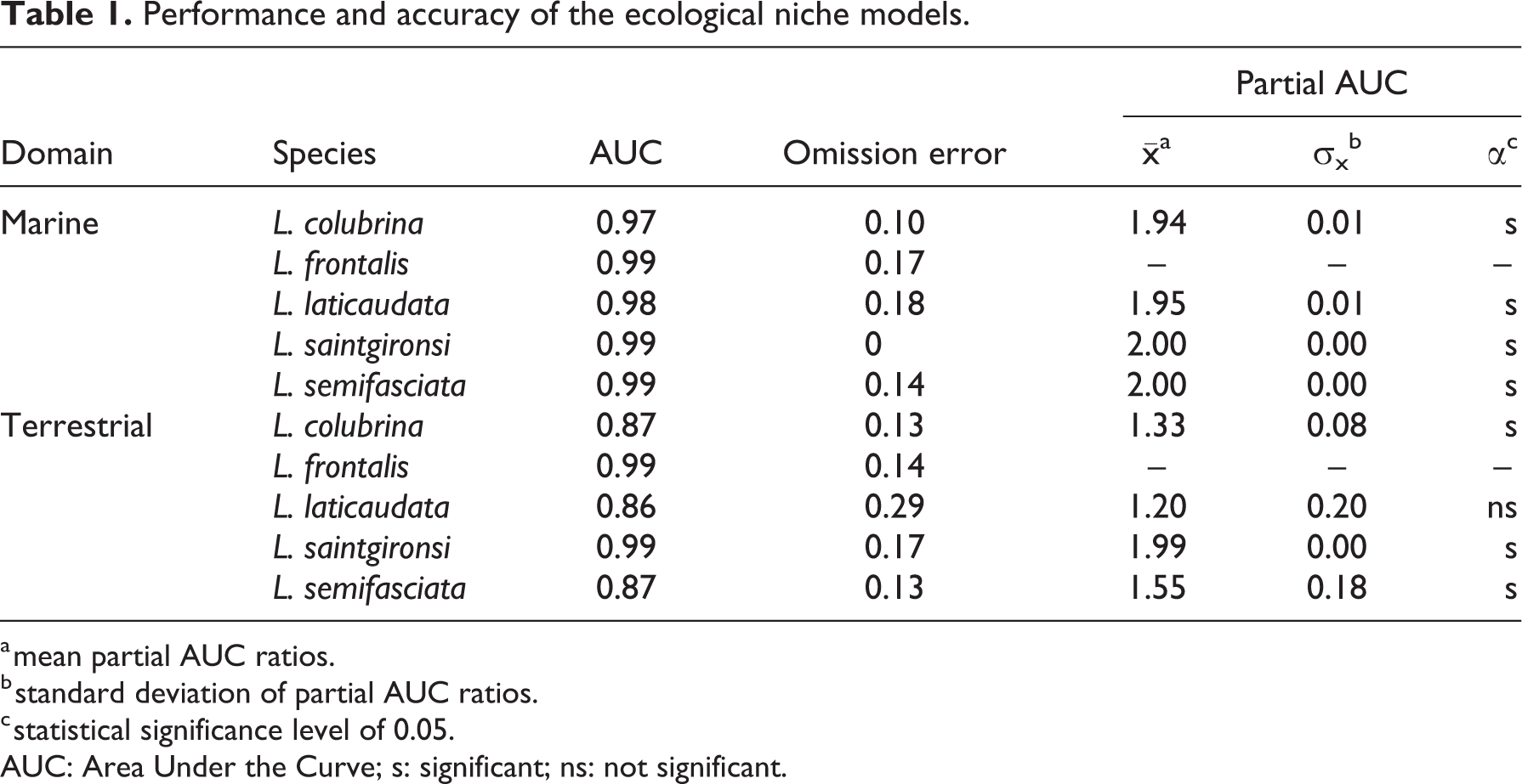
^a mean partial AUC ratios.

^b standard deviation of partial AUC ratios.

^c statistical significance level of 0.05.

AUC: Area Under the Curve; s: significant; ns: not significant.

3 Dispersal models

To estimate the dispersal of sea kraits across the study region, we used the cost distance analysis tool from ArcGIS 10.2. This tool calculates the resistance to dispersal from a known sea krait occurrence to the edge of the study region based on a cost raster (ESRI, 2011). We generated a cost raster that included three seascape features known to influence the dispersal of sea kraits: distance from the shoreline, water depth, and presence or absence of coral reefs and mangrove forests. The seasonal changes in the direction of sea currents as well as paleogeography changes of the area have had an impact on the distribution of sea krait species (Heatwole et al., 2017). However, because of the dynamic nature of these changes, we did not include them in the current analysis due to limited available data. We categorized the three variables for species’ dispersal ability using expert opinion (authors FB and IG) (Appendix 1), based on previously published data (Brischoux et al., 2009; Brischoux et al., 2013; Heatwole, 1999; Heatwole et al., 2005; Heatwole et al., 2012), and averaged the weighted variables in the final cost surface. The weighting was done on a scale from 0 to 100, on which 100 was given to seascape features known to inhibit sea krait mobility (e.g. sea kraits cannot feed on the seafloor deeper than 100 m below sea level), and 0 to seascape features known to be preferred by the sea kraits (e.g. coral reefs). The final cost raster represented the average ranking of the three weighted variables (Appendix 1). This cost raster and the occurrence points for each species were used as factors in the cost distance analysis in ArcGIS 10.2 (ESRI, 2011). We obtained a continuous raster (hereafter referred to as a dispersal raster) with smaller values representing high dispersal potential and larger values representing low dispersal potential (ESRI, 2011). To simplify the interpretation of the dispersal raster, we converted it to a binary form (dispersal and no dispersal) using the smallest value of the raster that comprised all species’ occurrence points as the threshold for defining dispersal. In context of species’ potential distributions estimated with ENM, the accessible area will define the range of the potential distribution to which species can disperse and occupy. The proportion of pixels (raster cells) from each suitability category (not suitable, suitable only in the terrestrial domain, suitable only in the marine domain, and suitable in both domains) within and outside of the accessible area was calculated for each sea krait in SAS JMP 10.

III Results

Of the total study region, we found that the proportion of area estimated by our dispersal models to be accessible to sea kraits was very small (Figure 1). For widespread sea krait species (L. colubrina, L. laticaudata, and L. semifasciata), the accessible areas were generally between 10% and 22% of the study region (Figure 1). However, endemic species with a narrow distribution range (L. frontalis and L. saintgironsi) could potentially access only 0.22% and 0.16%, respectively, of the study area (Figure 1).

Figure 1.

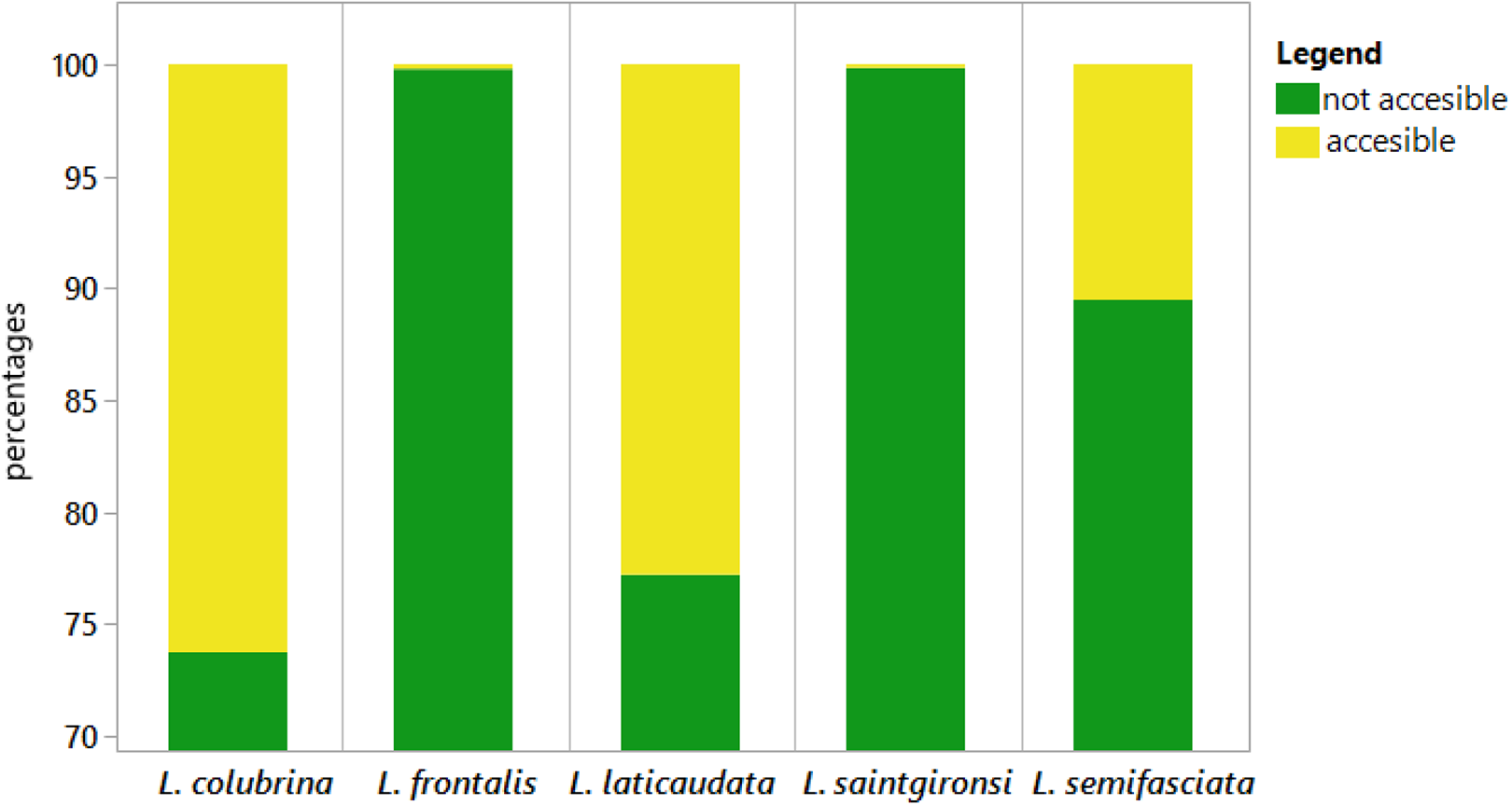
Proportion of environmentally suitable area (estimated with ecological niche modeling) within and outside of dispersal range for each sea krait species, determined with cost analysis.

By analyzing the suitability of the study region within and outside of the accessible area, we found that outside of the accessible area most of the pixels (>99%) were predicted as being unsuitable, whereas a very small proportion of pixels were in either category of suitability (terrestrial or marine, see Figure 2). All species showed the same trend, regardless of the extent of their accessible area within the study region (Figure 2). Regions outside of the accessible area that were suitable in both marine and terrestrial domains counted for less than 0.8% of the total number of pixels among all species (Figure 2). Moreover, in the case of L. frontalis and L. saintgironsi, less than 0.0001% of the region outside of their accessible area was predicted by the models as being suitable in both marine and terrestrial domains.

Figure 2.

Proportion of environmental suitability classes (based on ecological niche modeling) for each sea krait species in regions outside of dispersal range, estimated with cost analysis.

The region within the accessible area was found to be mostly unsuitable (70%–95% unsuitable) (Figure 3). On average, 4% of the pixels were suitable in both environments (marine and terrestrial); species with the least proportion of pixels accessible in both environments were L. laticaudata (0.45%) and L. semifasciata (0.6%) (Figure 3). This result suggests that, despite the two species’ wide potential distributions, the areas that are actually accessible to them are very small. Laticauda colubrina is the only widely distributed sea krait species that had more than 1% of suitable pixels in both marine and terrestrial environments within its accessible area (Figure 3). The species with the highest proportion of suitable areas within the accessible area were the endemic species: L. frontalis (2.8%); and L. saintgironsi (4.2%) (Figure 3).

Figure 3.

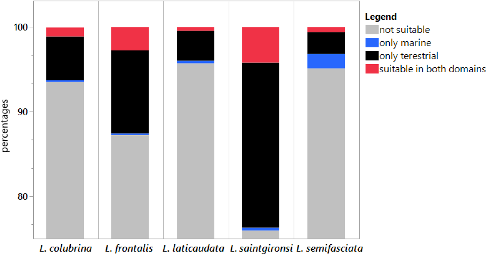
Proportion of environmental suitability classes (based on ecological niche modeling) for each sea krait species in areas inside of dispersal range, estimated with cost analysis.

Overall, most of the areas suitable for sea kraits were within the accessible area (Figure 4). Therefore, even though the overall proportion of suitable pixels within each species’ accessible area was relatively small, the majority of suitable pixels for each species occurred within the accessible area (Figure 4). For widely distributed species, most of the suitable pixels in the accessible area were in the terrestrial domain. Furthermore, within the area accessible to L. semifasciata, the proportion of suitable pixels in the terrestrial domain was larger than the proportion of suitable pixels predicted in both domains, compared with the whole study region (Figures 2, 3, and 4).

Figure 4.

Overview of potential distributions of sea kraits (based on ecological niche modeling) in relation to species specific dispersal range, estimated with cost analysis. The percentages represent the proportion of pixels (from entire potential distribution) for each suitability class that overlaps with the dispersal range for each species.

The distribution patterns of each species’ accessible area generally followed the coasts of the archipelagoes and nearby continents (Figure 5). In the case of Laticauda frontalis and L. saintgironsi, their accessible area was limited to the islands where they are known to occur (Figure 5). Extensive suitable areas were predicted for L. frontalis; however, these areas were not included in the accessible area, suggesting that this species may also be limited by its dispersal capabilities (Figures 4 and 5). However, most of the potential distribution for L. colubrina and L. saintgironsi was included within the accessible area (Figures 4 and 5), so we can assume that these species had already colonized most of their suitable areas.

Figure 5.

The estimated dispersal range (with cost analysis) and the potential distribution of each sea krait species (based on ecological niche modeling). Dispersal range is shown in yellow; outside of dispersal range is green; suitability in terrestrial domain is black; suitability in marine domain is blue; and suitability in both marine and terrestrial domains is red. For interpretation of the references to colours in this figure legend, refer to the online version of this article.

IV Discussion

Understanding species’ distributions still represents a challenging endeavor in biogeographical research. Starting with Wallace’s division of zoogeographical regions (Huxley, 1868; Mayr, 1944; Whitmore, 1982) right up to the present day, biogeographers have tried to unlock the code behind species’ distributions at large scales using various tools, from simple observations of species and creating distribution maps (Elfes et al., 2013; Sillero et al., 2014), to generating species’ distribution estimates by quantifying associations between species’ occurrences and corresponding environmental conditions (Peterson et al., 2011). ENM has been used extensively in the past decade to estimate species’ potential distributions (Mueller et al., 2013). However, as a relatively young field of study, ENM methods have some limitations, among them the selection of a study area extent for model training and the assumption that the entire study area is accessible to the species. In a recent article, Sahlean et al. (2014) showed that in the context of climate change, the Caspian whip snake will not be able to disperse across the study area within 70 years, a time span corresponding to the climate change scenarios. Therefore, even if new areas become suitable under future climate scenarios, some species may probably be unable to disperse to these areas (Sahlean et al., 2014). A similar problem exists for studies focusing on current distribution predictions in cases in which the area includes regions that cannot be reached by the organism due to dispersal limitations. In our study, we address this problem by proposing the use of a cost distance function to predict species’ dispersal across the study area.

1 Species’ distribution predictions in the context of dispersal

Of the study area we considered, only a small proportion (<26%) was estimated to be accessible to sea kraits (Figure 1). Moreover, for several species, less than 1% of the study region was accessible (Figure 1). Interestingly, the region outside of the area accessible to sea kraits was mostly predicted unsuitable, with only 0.16% of the pixels predicted suitable (Figure 2). For some species (L. saintgironsi and L. colubrina), up to 96% of the pixels predicted as suitable across the study region are accessible to the species (Figure 4). These results show that, overall, sea kraits seem to occupy most of their suitable available niche and that they may be unable to colonize much of the area outside of their dispersal ranges. Therefore, using dispersal estimates to refine species’ distribution predictions is a useful tool not only for refining the area of focus when ENM results are interpreted, but also for evaluating whether the studied species occupy the entire available suitable niche, or if they are limited by their dispersal capabilities.

2 Cost distance models in ENM studies

Cost distance models are widely available in both open-source (e.g. GRASS, Quantum GIS, R package “gdistance”) (Neteler et al., 2012; Quantum GIS Development Team, 2012; Van Etten, 2012) and proprietary software (e.g. ESRI ArcGIS) (ESRI, 2011). Therefore, cost distance analysis, or other distance-based methods to estimate species’ dispersal, can be done in a variety of software environments, depending on the researcher’s previous experience and software availability. Because the analysis itself uses a cost raster, which characterizes the landscape/seascape features that might influence species’ dispersal (Beier et al., 2009), factors that may not be used or are irrelevant from an ENM perspective can be incorporated. Generally, but depending on the question, cost rasters integrate features that might affect species’ dispersal, such as land cover or different types of barriers (lakes, rivers, or mountains) (see Beier et al., 2009; Urban and Keitt, 2001; Urban et al., 2009; for some examples, see Richard and Armstrong, 2010; Sahlean et al., 2014; Sawyer et al., 2011), as well as other data types that are freely available online (for a short review, see Sillero and Tarroso, 2010). An important limitation of cost distance models is that the cost raster is produced by ranking the dispersal resistance of the landscape/seascape features based on expert opinion (Beier et al., 2009; Richard and Armstrong, 2010). However, cost distance function is robust to potential landscape weighting errors and variables (Beier et al., 2009). Here, we used sea kraits, and we estimated dispersal over the ocean; however, our approach can be used for species that disperse over land. The application of this method to ENM research has great potential for estimating and visualizing the accessible area within the study region for both marine and terrestrial organisms.

3 Assessing commission error using estimates of accessible areas

The potential distributions obtained with ENM are subject to two types of errors: commission and omission (for details, see Anderson et al., 2003). Omission error is a type 2 statistical error, in which species’ known occurrence data are predicted as absent by the ENM estimates (Anderson et al., 2003). Omission error is usually easy to calculate because species’ presence data can be set aside from training the models and used to test them (Peterson et al., 2011). On the other hand, commission error is a type 1 statistical error, in which known absences are incorrectly predicted as present by the ENM (Anderson et al., 2003). Commission error is more difficult to estimate because: (a) it is challenging to determine whether an absence point is a “true absence” (Anderson et al., 2003); and (b) current ENM methods have been addressing the first problem and do not use “true absence” data when training the models (Peterson et al., 2011). Generally, it is accepted that commission error is less of a problem when the objective is to estimate the species’ potential distributions (Peterson et al., 2011). However, in some applications of ENM, commission error (represented by overprediction) has been a source of concern, especially when the models are transferred across space (to other geographical regions) or projected in time (under past or future conditions) (Peterson et al., 2011; Williams and Jackson, 2007). Areas predicted as suitable outside of the species’ dispersal ability also represent model overprediction. Hence, we can assume that by estimating species’ dispersal via cost analysis, the model overprediction due to dispersal limitations can be taken into account. In the case of our models for sea krait species, the overprediction accounted for less than 1%, because less than 1% of the region outside the accessible area was predicted suitable in both marine and terrestrial domains (Figure 2).

This simple method of estimating species’ dispersal can also help evaluate the ability of the models to predict the species’ distributions in areas that are not accessible to the species and, hence, the potential commission error represented by overprediction. Moreover, it can be used for any species, in both marine and terrestrial environments.

Footnotes

Acknowledgements

Authors with to express their gratitude to Dr. Arpad Nyari, Dr. Harold Heatwole and Dr. Stanley Fox for their help and useful suggestions that significantly improved our manuscript. We also wish to thank the anonymous reviewers that provided thoughtful feedback.

Declaration of conflicting interests

The author(s) declared no potential conflicts of interest with respect to the research, authorship, and/or publication of this article.

Funding

The author(s) received no financial support for the research, authorship, and/or publication of this article.

ORCID iD

Iulian Gherghel

Appendix 1

References

Anderson

Lew

Peterson

(2003) Evaluating predictive models of species’ distributions: Criteria for selecting optimal models. Ecological Modelling 162(3): 211–232.

Barve

Jimenez-Valverde

, et al. (2011) The crucial role of the accessible area in ecological niche modeling and species distribution modeling. Ecological Modelling 222(11): 1810–1819.

Beier

Majka

Newell

(2009) Uncertainty analysis of least-cost modeling for designing wildlife linkages. Ecological Applications 19(8): 2067–2077.

Bonnet

Ineich

Shine

(2005) Terrestrial locomotion in sea snakes: The effects of sex and species on cliff-climbing ability in sea kraits (Serpentes, Elapidae, Laticauda). Biological Journal of the Linnean Society 85(4): 433–441.

Brischoux

Bonnet

Legagneux

(2009) Are sea snakes pertinent bio-indicators for coral reefs? A comparison between species and sites. Marine Biology 156(10): 1985–1992.

Brischoux

Bonnet

Shine

(2007) Foraging ecology of sea kraits Laticauda spp. in the Neo-Caledonian Lagoon. Marine Ecology Progress Series 350: 145–151.

Brischoux

Bonnet

Shine

(2011) Conflicts between feeding and reproduction in amphibious snakes (sea kraits, Laticauda spp.). Austral Ecology 36(1): 46–52.

Brischoux

Tingley

Shine

, et al. (2012) Salinity influences the distribution of marine snakes: implications for evolutionary transitions to marine life. Ecography 35(11): 994–1003.

Brischoux

Tingley

Shine

, et al. (2013) Behavioral and physiological correlates of the geographic distributions of amphibious sea kraits (Laticauda spp.). Journal of Sea Research 76: 1–4.

10.

Brown

Kodric-Brown

(1977) Turnover rates in insular biogeography: Effect of immigration on extinction. Ecology 58(2): 445–449.

11.

Cooper

Soberon

(2018) Creating individual accessible area hypotheses improves stacked species distribution model performance. Global Ecology and Biogeography 27(1): 156–165.

12.

Elfes

Livingstone

Lane

, et al. (2013) Fascinating and forgotten: The conservation status of the world’s sea snakes. Herpetological Conservation and Biology 8(1): 37–52.

13.

ESRI (2011) ArcGIS Desktop: Release 10. 10th ed. Redlands, CA: Environmental Systems Research Institute.

14.

Flory

Kumar

Stohlgren

, et al. (2012) Environmental conditions associated with bat white-nose syndrome mortality in the north-eastern United States. Journal of Applied Ecology 49(3): 680–689.

15.

Franklin

(2009) Mapping species distributions: Spatial inference and prediction. Cambridge, UK: Cambridge University Press.

16.

Fuller

Munguía

Mayfield

, et al. (2006) Incorporating connectivity into conservation planning: A multi-criteria case study from central Mexico. Biological Conservation 133(2): 131–142.

17.

Gherghel

Brischoux

Papes

(2018) Using biotic interactions in broad-scale estimates of species’ distributions. Journal of Biogeography 45(9): 2216–2225.

18.

Gherghel

Papes

Brischoux

, et al. (2016) A revision of the distribution of sea kraits (Reptilia, Laticauda) with an updated occurrence dataset for ecological and conservation research. Zookeys 569: 135–148.

19.

Greer

(1997) The biology and evolution of Australian snakes. Sydney, Australia: Surrey Beatty.

20.

Heatwole

(1999) Sea Snakes. Malabar, USA: Krieger Publishing Company.

21.

Heatwole

Busack

Cogger

(2005) Geographic variation in sea kraits of the Laticauda colubrina complex (Serpentes: Elapidae: Hydrophiinae: Laticaudini). Herpetological Monographs 19(1): 1–136.

22.

Heatwole

Grech

Marsh

(2017) Paleoclimatology, paleogeography, and the evolution and distribution of sea kraits (Serpentes; Elapidae; Laticauda). Herpetological Monographs 31(1): 1–17.

23.

Heatwole

Grech

Monahan

, et al. (2012) Thermal biology of sea snakes and sea kraits. Integrative and Comparative Biology 52(2): 257–273.

24.

Heatwole

Lillywhite

Grech

(2016) Physiological, ecological, and behavioural correlates of the size of the geographic ranges of sea kraits (Laticauda; Elapidae, Serpentes): A critique. Journal of Sea Research 115: 18–25.

25.

Huxley

(1868) On the classification and distribution of the Alectoromorphae and Hetermorphae. Proceedings of the Zoological Society: 294–319.

26.

Jackson

Robertson

(2011) Predicting the potential distribution of an endangered cryptic subterranean mammal from few occurrence records. Journal for Nature Conservation 19(2): 87–94.

27.

Jimenez-Valverde

(2014) Threshold-dependence as a desirable attribute for discrimination assessment: Implications for the evaluation of species distribution models. Biodiversity and Conservation 23(2): 369–385.

28.

LaRue

Nielsen

(2008) Modelling potential dispersal corridors for cougars in midwestern North America using least-cost path methods. Ecological Modelling 212(3–4): 372–381.

29.

Lillywhite

Babonis

Sheehy

, et al. (2008) Sea snakes (Laticauda spp.) require fresh drinking water: Implication for the distribution and persistence of populations. Physiological and Biochemical Zoology 81(6): 785–796.

30.

Mayr

(1944) Wallace’s Line in the light of recent zoogeographic studies. The Quarterly Review of Biology 19(1): 1–14.

31.

Mesquita

PCMD

Pinheiro-Mesquita

Pietczak

(2013) Are common species endangered by climate change? Habitat suitability projections for the royal ground snake, Liophis reginae (Serpentes, Dipsadidae). North-Western Journal of Zoology 9(1): 51–56.

32.

Mueller

Baum

Papes

, et al. (2013) Potential ecological distribution of Cytauxzoon felis in domestic cats in Oklahoma, Missouri, and Arkansas. Veterinary Parasitology 192(1-3): 104–110.

33.

Neteler

Bowman

Landa

, et al. (2012) GRASS GIS: A multi-purpose open source GIS. Environmental Modelling & Software 31: 124–130.

34.

Nyári

ÁS

Reddy

(2013) Comparative phyloclimatic analysis and evolution of ecological niches in the Scimitar Babblers (Aves: Timaliidae: Pomatorhinus). PLOS ONE 8(2): e55629.

35.

Park

Kim

Fong

, et al. (2017) Northward dispersal of sea kraits (Laticauda semifasciata) beyond their typical range. PLOS ONE 12(6): e0179871.

36.

Peterson

Soberon

(2012) Species distribution modeling and ecological niche modeling: Getting the concepts right. Natureza & Conservacao 10(2): 102–107.

37.

Peterson

Benz

Papeş

(2007) Highly pathogenic H5N1 avian influenza: Entry pathways into North America via bird migration. PLOS ONE 2(2): e261.

38.

Peterson

Papeş

Kluza

(2003) Predicting the potential invasive distributions of four alien plant species in North America. Weed Science 51(6): 863–868.

39.

Peterson

Soberón

Pearson

, et al. (2011) Ecological Niches and Geographic Distributions. Princeton, NJ: Princeton University Press.

40.

Phillips

Dudik

Schapire

(2004) A maximum entropy approach to species distribution modeling. In: Proceedings of the 21st International Conference on Machine Learning (eds. Koller

Schuurmans

Bengio

Bottou

), Banff, Alberta, Canada, 4–8 July 2004, 655–662. ACM Press.

41.

Psonis

Antoniou

Karameta

, et al. (2018) Resolving complex phylogeographic patterns in the Balkan Peninsula using closely related wall-lizard species as a model system. Molecular Phylogenetics and Evolution 125: 100–115.

42.

Pyron

Burbrink

Colli

, et al. (2011) The phylogeny of advanced snakes (Colubroidea), with discovery of a new subfamily and comparison of support methods for likelihood trees. Molecular Phylogenetics and Evolution 58(2): 329–342.

43.

Quantum GIS Development Team (2012) Quantum GIS geographic information system. Available at: https://qgis.org/en/site/ (accessed 24 September 2019).

44.

Reed

Shine

Shetty

(2002) Sea kraits (Squamata: Laticauda spp.) as a useful bioassay for assessing local diversity of eels (muraenidae, congridae) in the western Pacific Ocean. Copeia 2002(4): 1098–1101.

45.

Richard

Armstrong

(2010) Cost distance modelling of landscape connectivity and gap-crossing ability using radio-tracking data. Journal of Applied Ecology 47(3): 603–610.

46.

Roberts

Hamann

(2012) Predicting potential climate change impacts with bioclimate envelope models: A palaeoecological perspective. Global Ecology and Biogeography 21(2): 121–133.

47.

Sahlean

Gherghel

Papes

, et al. (2014) Refining climate change projections for organisms with low dispersal abilities: A case study of the Caspian whip snake. PLOS ONE 9(3): e91994.

48.

Sarkar

Sanchez-Cordero

Londono

, et al. (2009) Systematic conservation assessment for the Mesoamerica, Choco, and Tropical Andes biodiversity hotspots: A preliminary analysis. Biodiversity and Conservation 18(7): 1793–1828.

49.

Saupe

Papes

Selden

, et al. (2011) Tracking a medically important spider: Climate change, ecological niche modeling, and the brown recluse (Loxosceles reclusa). PLOS ONE 6(3): e17731.

50.

Sawyer

Epps

Brashares

(2011) Placing linkages among fragmented habitats: Do least-cost models reflect how animals use landscapes? Journal of Applied Ecology 48(3): 668–678.

51.

Shetty

Shine

(2002a) The mating system of yellow-lipped sea kraits (Laticauda colubrina: Laticaudidae). Herpetologica 58(2): 170–180.

52.

Shetty

Shine

(2002b) Philopatry and homing behavior of sea snakes (Laticauda colubrina) from two adjacent islands in Fiji. Conservation Biology 16(5): 1422–1426.

53.

Sillero

Tarroso

(2010) Free GIS for herpetologists: Free data sources on Internet and comparison analysis of proprietary and free/open source software. Acta Herpetologica 5(1): 63–85.

54.

Sillero

Campos

Bonardi

, et al. (2014) Updated distribution and biogeography of amphibians and reptiles of Europe. Amphibia-Reptilia 35(1): 1–31.

55.

Urban

Keitt

(2001) Landscape connectivity: A graph-theoretic perspective. Ecology 82(5): 1205–1218.

56.

Urban

Minor

Treml

, et al. (2009) Graph models of habitat mosaics. Ecology Letters 12(3): 260–273.

57.

Vaclavik

Meentemeyer

(2012) Equilibrium or not? Modelling potential distribution of invasive species in different stages of invasion. Diversity and Distributions 18(1): 73–83.

58.

Van Etten

(2012) R package gdistance: Distances and routes on geographical grids. Version 1.1-4. Available at: http://citeseerx.ist.psu.edu/viewdoc/download?doi=10.1.1.368.305&rep=rep1&type=pdf (accessed 24 September 2019).

59.

Vidal-Garcia

Serio-Silva

(2011) Potential distribution of Mexican primates: Modeling the ecological niche with the maximum entropy algorithm. Primates 52(3): 261–270.

60.

Whitmore

(1982) Wallace’s Line: A result of plate tectonics. Annals of the Missouri Botanical Garden 69(3): 668–675.

61.

Wiens

Graham

(2005) Niche conservatism: Integrating evolution, ecology, and conservation biology. Annual Review of Ecology Evolution and Systematics 36(1): 519–539.

62.

Williams

Jackson

(2007) Novel climates, no-analog communities, and ecological surprises. Frontiers in Ecology and the Environment 5(9): 475–482.