



Abstract
In this paper, we develop an improved outlier pointwise elimination rule based on the wind-power observation data and prove that when the stopping-parameter is
Introduction
For the past few years, the technology of wind power has been developed and is relatively mature, and the proportion of wind energy in the power grid shows a rising trend. However, the characteristics of wind such as intermittent, volatile and low energy density (Wang et al., 2011; Yao et al., 2011) always lead to intermittent and volatile power generation, which increases the difficulty of dispatching and the requirement of network preparation dosage (Wang et al., 2009). Therefore, developing wind-power research actively to improve the accuracy of forecasting has a realistic significance on dispatching and reducing the operation cost of the system (Yang et al., 2005).
There are lots of wind power forecasting models such as the time series analysis method (Liu et al., 2013; Qing and Yang, 2014), the neural network method (Sideratos and Hatziargyriou, 2007), the Kalman filtering method (Cassola and Burlando, 2012; Xiu and Guo, 2013), wavelet analysis (Grinstead et al., 2004; Tai et al., 2003), etc. In 2008, Pan Yifu developed a mixture forecasting model by integrating a time series with the Kalman filter, which could solve the problem of time delay and mine the regulation among dynamic data greatly. However, the defect is that the forecasting results are non-ideal when there are large leaps among the data.
What’s more, fewer models have considered the effects of abnormal observation data on the accuracy of a model, for example, it would lead to a large deviation from realistic results. In order to improve the accuracy of the forecast, it is necessary to eliminate the abnormal data first. In 1997, Wang Zhengming developed the one-by-one method of outlier rejection in a linear regression model. Nevertheless, the fact is that the observation data usually show the characteristic of a nonlinear relationship.
In this paper, we research a pointwise elimination method for the abnormal data of wind power based on the nonlinear model, and we obtain a criterion of stopping-rule. Furthermore, we propose the exponential smoothing method which considers the factor of trend to amend the large leaps among the data, and we develop an improved short-term forecasting model, which has a high accuracy. Finally, a numerical experiment shows the effectiveness of our model based on the data from some power supply companies.
This paper is divided into three sections. In the next section, we develop the pointwise elimination method for the abnormal data under the nonlinear model and show an improved stopping-rule. In the third section, we obtain an improved short-term forecasting model which integrates the exponential smoothing method with a time series and the Kalman filter. In the last section, a numerical experiment shows simulation results and illustrates the effectiveness of our method.
Outlier pointwise elimination method
Generally, there will inevitably exist some abnormal observation data among statistical data and it would have a negative impact on wind-power forecasting results. For the purpose of reducing the errors of forecast, it is very important to detect and eliminate the abnormal observation data.
Considering the nonlinear model

where
Let
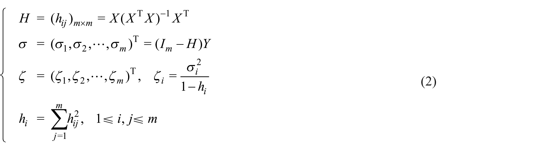


where
Lemma 2.1 shows that the greater the value of

For a given stopping-parameter
According to Lemma 2.2, the stopping-parameter

where
Let

we have

From equations (4) and (5), there exists the test statistic

where
From equation (2), rewriting

Combined with equations (6) and (7) and Lemma 2.1, we obtain

By equation (8) and Lemma 2.2, it follows that

Thus, it is obvious that equation (9) satisfies

then we have

which implies that

This completes the proof of Theorem 2.1.
Improved short-term forecasting model
In this section, we research a low order Auto-Regressive and Moving Average Model (ARMA) which is a time series model and can reflect the signal variation. Under the prediction equation from the ARMA model, the Kalman filtering state equation and measurement equation can be deduced. Then, we take advantage of the Kalman filtering prediction iterative equation to forecast. In order to reduce the errors, we utilize the exponential smoothing method to smooth the large leaps among the data before forecasting.
The ARMA time series forecasting
Let

where
Applying operators

where the solutions of
Considering the Augmentation Dickey–Fuller(ADF) testing model

where ∆xt is the first-order difference series,
After testing, we estimate the parameters of the prediction equation of the ARMA model through the maximum likelihood estimation.
The fundamental of Kalman filtering
The Kalman filtering method describes the filter through the state space model of the linear stochastic system which is composed of the state equation and observation equation. Besides, it utilizes the recurrence properties of the state equation and the linear unbiased minimum variance estimation criterion to estimate the state variable of filter optimally.
The general linear discrete system is denoted as


where
Mixture forecasting model based on ARMA with Kalman filter
Through converting the model (10) into state space, we would obtain the state equation and the measurement equation of the Kalman filter.
First, we rewrite equation (10) as

where
Then, we convert equation (15) into the state space model

where







and
Improvement of the model
In general, the forecasting results of the mixture model have been satisfactory. However, facing the large leaps among data, the results would be non-ideal. Hence we take advantage of the three times exponential smoothing method, which considers the factor of trend to amend the large leaps among the data, and integrate it with the mixture model to develop an improved short-term forecasting model.
Considering the three times exponential smoothing moving model


where
In fact, the rising or falling trend of some parts of the data will lead to the forecast behind the actual trend. Thus, we introduce the trend factor into the model equation (17).
The adjusted model is


where
A numerical example
In this experiment, we take the wind-power data per five minutes (216 in all) from some wind farms in Zhejiang province on January 1, 2009 as the research object.
First of all, we conduct the three order polynomial fitting on the data per hour, and adopt Theorem 2.1 to eliminate the abnormal data. Figure 1 shows the fitting curve before and after elimination.

The fitting curves before and after elimination.
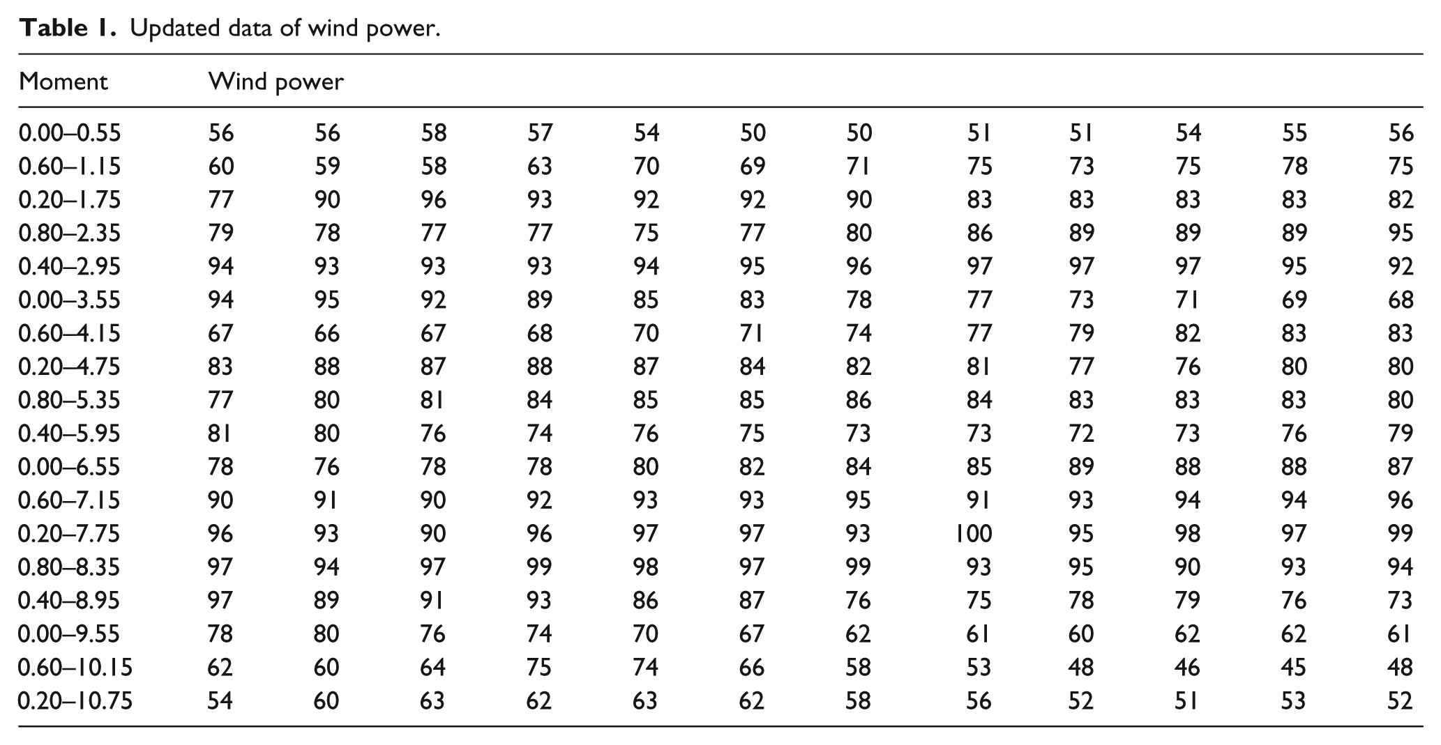
In accordance with the new fitting curve, we update the raw data (refer to Table 1). The trend curve of wind power (Figure 2) shows clearly that there exist some large leaps among the data. Thus, we apply the three times exponential smoothing method to optimize the data as a series
Updated data of wind power.
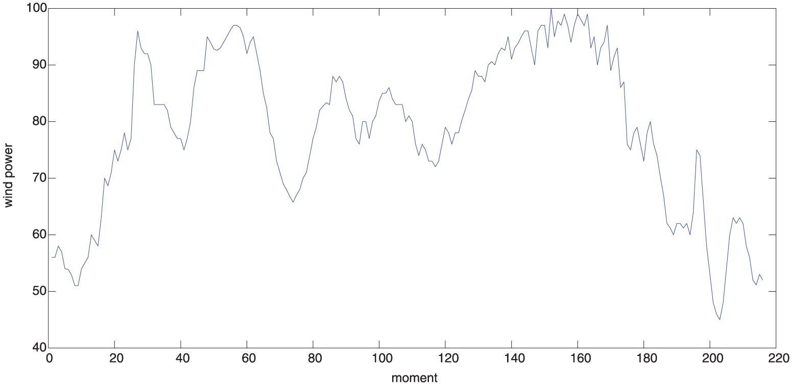
The trend curve of wind power.
Then, combining the first 20 autocorrelation coefficients of the sequence
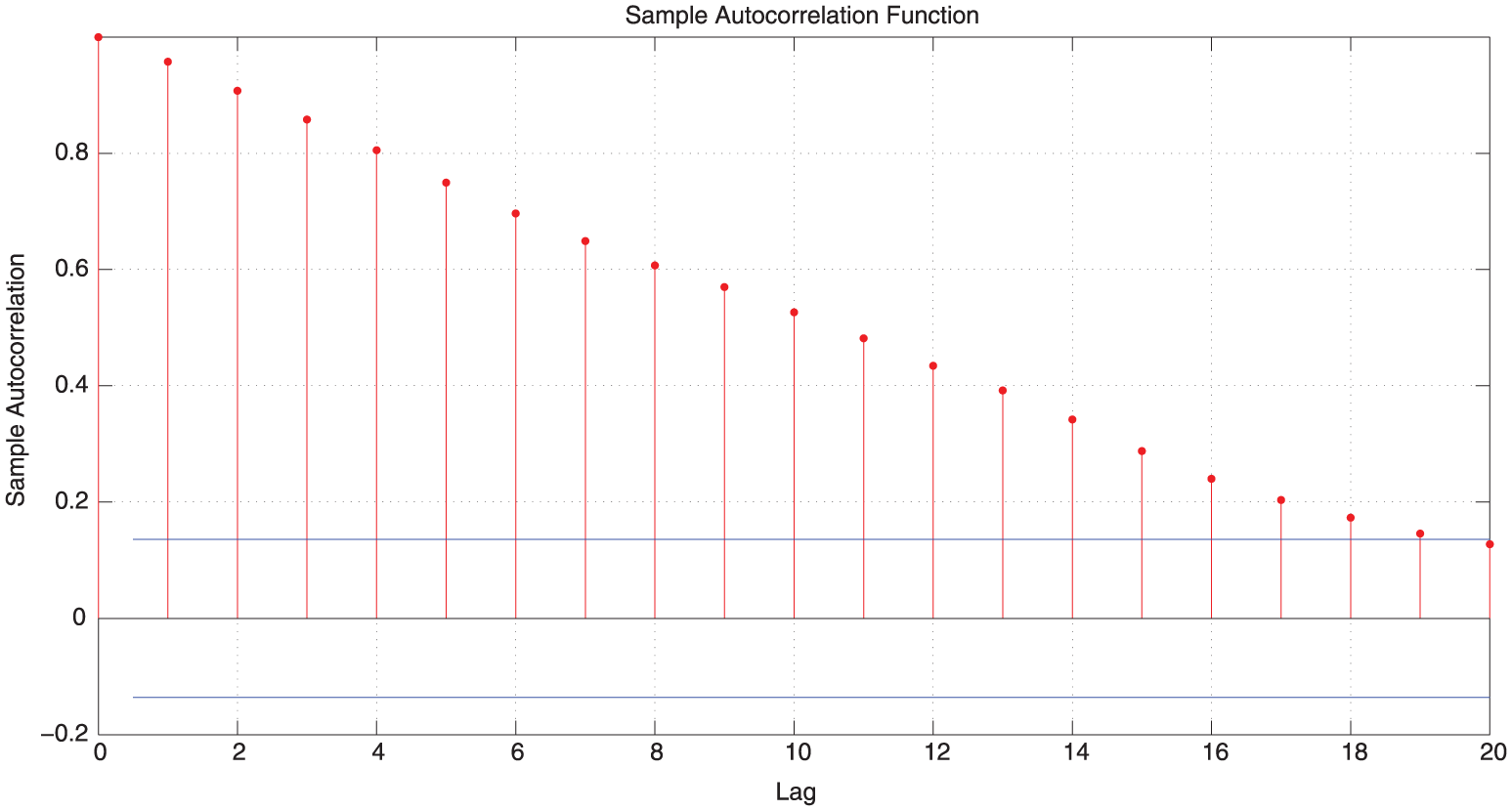
The first 20 autocorrelation coefficients of
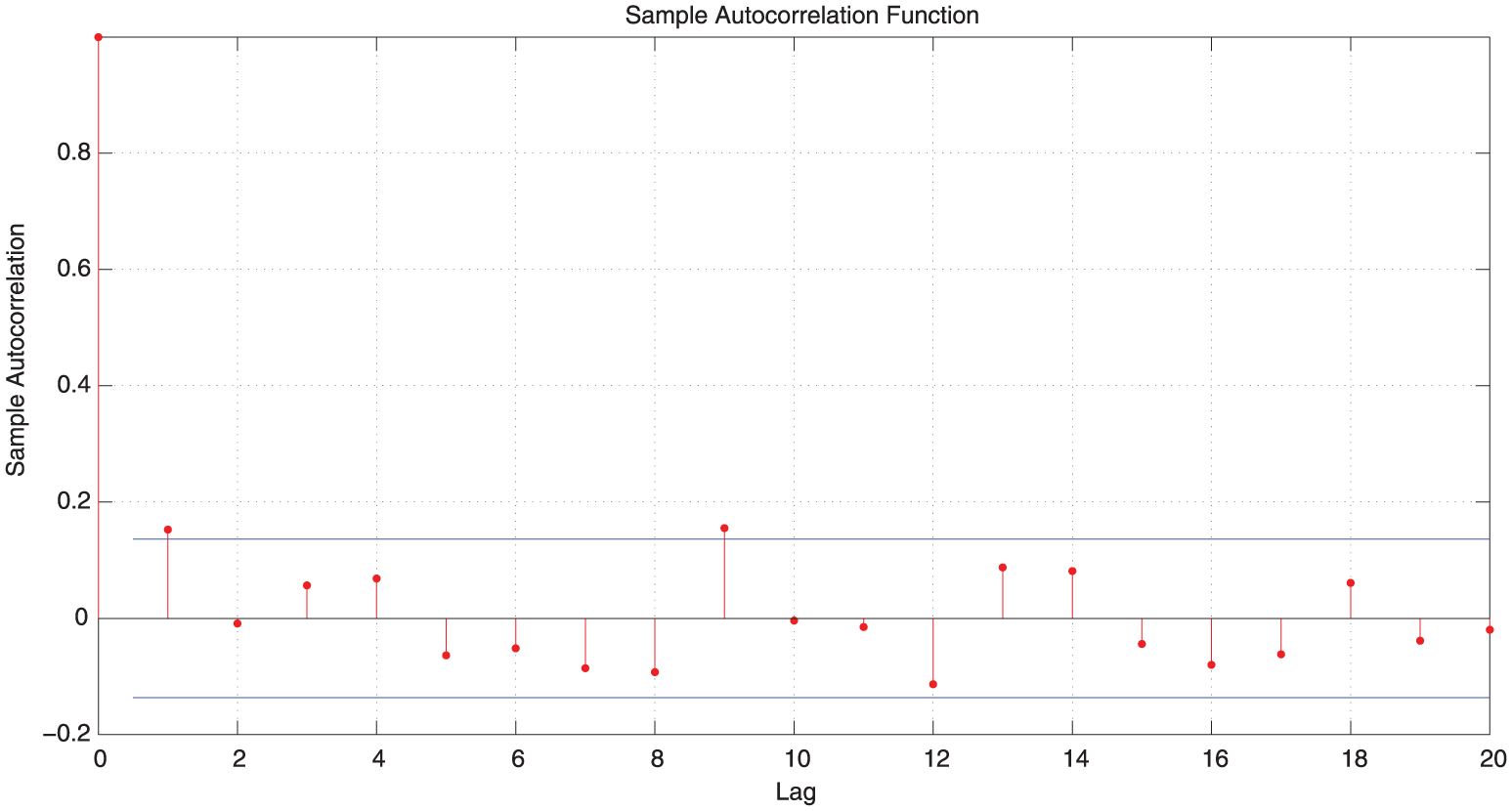
The first 20 autocorrelation coefficients of
Furthermore, the orders of model (10) could be identified as ARMA(3,2) by the Akaike information criterion (Akaike, 1974) and the parameters would be estimated by maximum likelihood method as follows

Let

Converting equation (18) into state space, we can get the state equation (19) and the measurement equation (20)
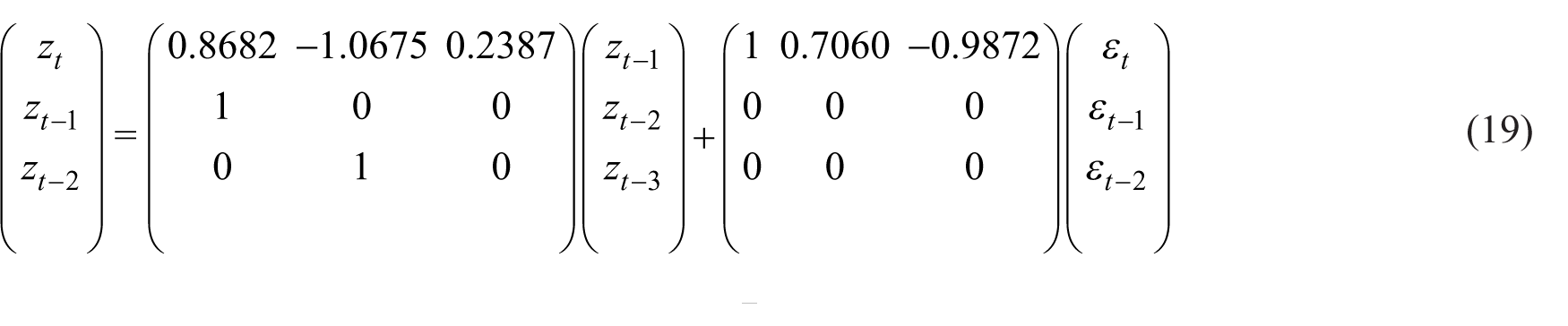

where
Finally, we realize the improved short-term forecasting model through MATLAB to forecast the data. Figure 5 shows the curves of the comparison between actual data and forecasting data for the next hour.

The wind-power forecasting result under the hybrid model.
The experiment shows the following.
1. The mixture model which integrates the time series with the Kalman filter can catch the dynamic regulation of wind-power data effectively. Based on the updated data, we can forecast the data for the next hour and get an error precision of 1.69%.
2. The mixture model does not fit the large variational data such as big leap points. It is effective to utilize the three times exponential smoothing method to improve the accuracy of the forecasting results. Under the improved short-term forecasting model, the error precision of the results can decrease to 0.94%
3. Although we can obtain high-precision results through the improved short-term forecasting model, the length of forecast is short. With the increase in the length of forecasting, the accuracy of results will decrease.
Footnotes
Declaration of conflicting interests
The author(s) declared no potential conflicts of interest with respect to the research, authorship and/or publication of this article.
Funding
The first and the second authors are supported by the Fundamental Research Funds for the Central Universities (No. 2015ZCQ-LY-01) and the National Natural Science Foundation of China (Grant No. 11501032). The third and the fourth authors are supported by the National Grid Project: Method for ultra short term wind power prediction based on temporal and spatial correlation of air flow field (No. SGTJ0000KXJS1400130).