Comparison of computational fluid dynamics and mass-conserving approaches for annual energy production (AEP) evaluation: Part I: analysis of a standard wake model and wind speed/power curve implementations

Abstract

A variety of microscale numerical approaches are available nowadays for high-resolution local flow characterization, differing on accuracy according to the application and on computational effort. In this study, a mass-conserving and a computational fluid dynamics wind flow model were compared using openWind and WindSim tools. The flow over an idealized terrain, perfectly flat with uniform surface roughness, was simulated with equivalent setup in both models to evaluate the implementation of turbine power curve and of a wake model, avoiding terrain effects. In this flat terrain, both approaches provided the same (uniform) speed-up field. Wind turbines were distributed over the domain in different arrays and spacing layouts. The power curve implementation, analyzed through gross annual energy production estimates, showed similar results in these tools. For net annual energy production, a maximum difference of 2.6% was found, showing small sensitivity regarding the same wake model implementation. The models herein employed may be considered equivalent for terrain-independent cases.

Keywords

Wind energy wind flow models computational fluid dynamics mass-conserving annual energy production

Introduction

Due to the increased demand for renewable sources of electricity, the wind energy sector has grown enormously worldwide in the past few years, as well as the researches about this topic (Kumar et al., 2016; Ramechecandane and Gravdahl, 2012).

Wind mapping is of utmost importance in several wind energy and wind engineering applications. Wind farms must be installed in sites of high wind potential to assure the profitability of the project. Due to the irregular availability of the wind resources, an accurate comprehension about its distribution over the area of interest is crucial to improve the energy yield prediction. Hence, the motivation of this study came from the need of improving tools for wind resource assessment.

Currently, numerical modeling of atmospheric flow is the main tool utilized for local flow distribution studies. These mathematical models are designed by integration of appropriate equations with adequate initial and boundary conditions. Limited computer capacity requires that various assumptions are made due to the complex non-linear nature of the equations, which can be simplified according to the problem to be represented, and there is often a compromise between time and computational cost and between physics and geometric complexity (Wakes et al., 2010).

In many cases, steady-state treatments are feasible for solving the time average flow and estimating turbulence statistics. Theoretically, this is valid when the region of the terrain under investigation is small enough so that the time required for an air particle to pass through the region is much smaller than the time over which meteorological synoptic-scale phenomena evolve (Prospathopoulos et al., 2012). Furthermore, steady-state solutions are adopted as a good estimate of the average of speed-up for a long-term velocity conversion.

In wind industry, microscale models have been increasingly employed to solve steady-state flow in order to obtain three-dimensional (3D) wind resource maps. In this context, they are used in projects of new wind farms for micrositing studies, since they can provide high-resolution wind maps and describe the wind pattern over the simulation area (Albani and Ibrahim, 2014; Ayotte, 2008; Blocken et al., 2015; Jafari et al., 2012; Rasouli and Hangan, 2013; Rodrigo, 2010; Simões and Estanqueiro, 2016; Timander and Westerlund, 2012). Different numerical approaches have been applied, but the most usual are linearized models (including mass-consistent) and computational fluid dynamics (CFD) models with different ways of turbulence modeling, like Reynolds-averaged Navier–Stokes (RANS) and large eddy simulation (LES)—more restricted application. All models attempt to solve at least some of the physical equations governing motions of the atmosphere, with varying degrees of complexity.

Depending on the extension of the study area, on the hypotheses adopted, and on which mathematical approach is applied, the stages of wind resource estimation and micrositing can be very time consuming. This is a challenge face to the demand of projects and the huge prosperity of the wind energy sector.

Still, wind farms are becoming increasingly large in size. Therefore, wake models are needed to quantify the wake losses that arise from the interactions between turbines in operation, caused by this clustered arrangement.

This study aims to evaluate some tools utilized in the wind industry for high-resolution local flow characterization. Two different microscale numerical models are compared over a flat terrain: a mass-conserving and a CFD RANS wind flow model, using the software openWind (WindMap; AWS Truepower, 2010) and WindSim (Meissner, 2015). There are numerous previous works that have compared different atmospheric boundary layer (ABL) modeling, such as Berge et al. (2006), Bechmann et al. (2011), Neophytou et al. (2011) and Timander and Westerlund (2012). In addition, Bitsuamlak et al. (2004) revised and compared studies carried out with different kinds of models for different topographies and parameters. However, they are usually addressed to wind farm studies, besides predominantly applied over complex terrains. On the other hand, this work is not intended to be compared to a wind farm project, but only a study of models.

This article is part of a more general project that relies on investigating how different numerical methods are dependent on the relief. In this first part, the flow over a perfectly idealized flat terrain with an uniform surface roughness length has been simulated to analyze the terrain-independent genuine numerical methods. In this flat terrain, the two approaches provided the same speed-up field. Therefore, the target of this part of the work is to verify if there are differences in the wake model implementation and in the methods of turbine power curve modeling for annual energy production (AEP) calculation in these computational tools. The influence of the wake effect on the AEP estimations has been taken into account employing a standard analytical wake model, the “Jensen model.” Equivalent parameters were used in both models to assure a free tendency analysis, obtaining a comparison of their performances to proceed the second part of the ongoing study, where these two tools will be employed for micrositing of wind farms in a region with complex terrain surrounded by a large flat terrain, located in the northeast region of Brazil.

Mathematical modeling

Prospathopoulos et al. (2012) summarize that steady-state models may be divided into kinematic and dynamic models. Kinematic or mass-consistent models solve only the continuity equation assuming inviscid fluid flow. They are very simple models and require low computational effort, but they cannot take into account the effect of turbulence or predict separation, so they are mainly used in large area applications to derive wind atlases. While dynamic models solve the continuity, the momentum and (possibly) the energy conservation equations and their degrees of complexity vary according to the manipulation of the terrain data, the simplifications in the equations, the turbulence model, and so on.

Due to its simplicity, mass-conserving models are generally applied for gentle terrain, being usually as capable as the others to reproduce neutral ABL wind fields, despite requiring much less computational cost (Ayotte, 2008; Gasset et al., 2012). On the other hand, dynamic models like CFD are generally stated to be suitable for high-resolution mapping of complex terrains (Bechmann et al., 2011; Bitsuamlak et al., 2004; Blocken et al., 2015; Rasouli and Hangan, 2013) due to the consideration of non-linearity. Nonetheless, Berge et al. (2006), Neophytou et al. (2011), Beaucage et al. (2014), and Castellani et al. (2015), for example, showed that, although in most cases CFD presents better results than the other more simplified models, this is not in the totality.

The numerical methodologies employed by the two wind flow models used in this study are presented hereafter.

Mass-conserving models

Mass-conserving models solve just one of the physical equations of motion to generate 3D terrain-dependent wind flow: the continuity equation. They do not enclose dynamic equations and the approach is simply to reach a divergence-free velocity field starting from wind observations.

The numerical procedure is based on an initial solution obtained by interpolating/extrapolating wind observations taken in one or more points inside the simulation domain into all the grid points, which is a first guess wind field. This is then altered according to the interferences caused by the local terrain (orography, roughness, and obstacles), giving an adjusted wind field $U_{0} (u_{0}, v_{0}, w_{0})$ . In sequence, $U_{0}$ is forced to be divergence free, giving the mass conservative wind field $U (u, v, w)$ (Bengtsson, 2015; Cataldo and Zeballos, 2009; Eriksson, 2013; Sherman, 1978).

The difference between U and U₀ should be as small as possible and the wind field of $U$ should be mass consistent which means that it should satisfy the physical principle of mass conservation (equation (1)), which represents the mass balance inside the control volume

\frac{\partial U_{j}}{\partial x_{j}} = \frac{\partial u}{\partial x} + \frac{\partial v}{\partial y} + \frac{\partial w}{\partial z} = 0

(1)

The functional $E (u, v, w, λ)$ shown in equation (2) minimizes the variance of the difference between the wind fields ( $U$ and $U_{0}$ ). The Lagrange multiplier (λ) is used to introduce the non-divergence wind velocity field condition, the mass conservation being the strong constraint (Cataldo and Zeballos, 2009; Eriksson, 2013). The constants $α$ and $β$ control the contribution of the horizontal and vertical wind speed components to the divergence

E (u, v, w, λ) = \int [α^{2} {(u - u_{0})}^{2} + α^{2} {(v - v_{0})}^{2} + β^{2} {(w - w_{0})}^{2} + λ (\frac{\partial u}{\partial x} + \frac{\partial v}{\partial y} + \frac{\partial w}{\partial z})] d V

(2)

The associated equations, the solution of which minimizes equation (2), are

u = u_{0} + \frac{1}{2 α^{2}} \frac{\partial λ}{\partial x}, v = v_{0} + \frac{1}{2 α^{2}} \frac{\partial λ}{\partial y}, w = w_{0} + \frac{1}{2 β^{2}} \frac{\partial λ}{\partial z}

(3)

Hence, by substituting equation (3) in equation (1), the Poisson equation (4) can be obtained. Equation (4) is iterated over the whole domain for each wind direction, according to correct boundary conditions. In case, $λ = 0$ is used to the open borders and $\partial λ / \partial n = 0$ to the solid boundaries (ground and top), where n is the normal coordinate to such surfaces

\frac{1}{2 α^{2}} (\frac{\partial^{2} λ}{\partial x^{2}} + \frac{\partial^{2} λ}{\partial y^{2}}) + \frac{1}{2 β^{2}} \frac{\partial^{2} λ}{\partial z^{2}} = - (\frac{\partial u_{0}}{\partial x} + \frac{\partial v_{0}}{\partial y} + \frac{\partial w_{0}}{\partial z}) = - \frac{\partial U_{0_{j}}}{\partial x_{j}}

(4)

Equation (4) is the same as equation (3) of Walmsley et al. (1990) and equation (3.12) of Bengtsson (2015), based on Phillips and Traci (1979). In WindMap, λ is referred to as the velocity potential (Φ) and $1 / 2 α^{2}$ and $1 / 2 β^{2}$ as $τ_{h}$ and $τ_{v}$ , respectively, that accounts for the deviation of the atmosphere from neutral conditions.

The software openWind, developed by AWS Truepower (2010), was used in this work in its Basic version as an interface to the WindMap tool, based on Numerical Objective Analysis of Boundary Layer (NOABL), developed in turn by Phillips and Traci (1979). The model was further improved to take into account internal boundary layer growth due to sharp transition in surface roughness (Brower, 1999).

CFD models

CFD consists of a numerical method for solving non-linear partial differential equations (PDEs) that represent a physical flow field. Through a discretization scheme, the continuum solution domain is transformed in a discrete problem with a finite number of nodal points. The PDEs are then integrated over the computational grid and transformed into a system of algebraic equations that is solved iteratively until a convergent solution is obtained according to the pre-established error criteria (Versteeg and Malalasekera, 2007).

CFD solves the RANS equations to simulate the flow field characteristics (velocity, pressure, and temperature). These models generate a basic wind field considering local terrain perturbations and standard inlet boundary conditions. Since they do not take into account the actual local speed values and velocity directions, the CFD results need to be adjusted according to the measurements taken inside the considered region.

CFD RANS equation solvers had an extensive development over the 70s and 80s and are considered for some authors as the scientifically most promising tool for computational simulation and even the state of the art in wind flow modeling (Bechmann et al., 2011; Sumner et al., 2010; Theodoropoulos and Deligiorgis, 2009).

The CFD calculations were performed in this study through the commercial software WindSim, version 7.0 (Meissner, 2015). It is a CFD package based on the more general PHOENICS solver (CHAM) and was developed in Norway in the 1990s to facilitate the detailed project of wind farms. Considering steady-state, incompressible flow and neutral atmospheric stratification, by default, the RANS equations are discretized and integrated on the computational grid through a finite volume method approach.

The mean flow is solved through the physical principles of conservation of mass and momentum. The former is presented in equation (1) and the latter is given by the Navier–Stokes equation (5)

U_{j} \frac{\partial U_{i}}{\partial x_{j}} = - \frac{1}{ρ} \frac{\partial p}{\partial x_{i}} + \frac{\partial}{\partial x_{j}} [ν (\frac{\partial U_{i}}{\partial x_{j}} + \frac{\partial U_{j}}{\partial x_{i}}) - (\bar{u_{i} u_{j}})]

(5)

expressing the balance of the transport of fluid due to pressure and viscosity forces. The variable $U$ is the velocity vector with its components, $ρ$ and $p$ are the constant air density and pressure, respectively, and $ν$ is the kinematic viscosity. The turbulent Reynolds stresses relate to the mean velocity variables through the turbulent viscosity $ν_{t}$

\bar{u_{i} u_{j}} = - ν_{t} (\frac{\partial U_{i}}{\partial x_{j}} + \frac{\partial U_{j}}{\partial x_{i}}) + \frac{2}{3} δ_{i j} k

(6)

The turbulence is parameterized through some closure model. The most common (and adopted in this work) is the standard k–ε, represented in the following equations

U_{j} \frac{\partial k}{\partial x_{j}} = \frac{\partial}{\partial x_{j}} (\frac{ν_{t}}{σ_{k}} \frac{\partial k}{\partial x_{j}}) + P_{k} - ε

(7)

U_{j} \frac{\partial ε}{\partial x_{j}} = \frac{\partial}{\partial x_{j}} (\frac{ν_{t}}{σ_{ε}} \frac{\partial ε}{\partial x_{j}}) + C_{ε 1} \frac{ε}{k} P_{k} - C_{ε 2} \frac{ε^{2}}{k}

(8)

ν_{t} = c_{μ} \frac{k^{2}}{ε}

(9)

where k and ε are the turbulent kinetic energy and its dissipation rate, respectively; P_k is the turbulent production term; and c_µ, $σ_{k}$ , $σ_{ε}$ , $C_{ε 1}$ , and $C_{ε 2}$ are the constants, the values of which vary according to each turbulence model (formulae based on Gravdahl, 1998).

The lateral inlet boundary condition in WindSim is defined by the logarithmic vertical wind profile, valid from the surface roughness length to the boundary layer height. Above this, the horizontal wind speed is constant, following the geostrophic wind approximation. The boundary condition used at the top was no-friction wall (recommended for flat terrain), but it can also be fixed pressure.

Wake models

The objective of a wake model is to assess the energy deficit in the downstream wind field, and not to describe the wind field properly. Analytical—or engineering—wake models use the wind field generated from the main numerical processing (in this case, from the CFD and mass-conserving models) to predict a velocity deficit usually on the wake centerline, which means that the calculation is independent. The model herein employed was formulated by Jensen (1983) and Katíc et al. (1986).

The Jensen model is well established and one of the most widely accepted by the wind energy industry, even though it is one of the oldest wake models still in use and limited to small wind farms (González et al., 2014; Seim, 2015; Shakoor et al., 2016). This model is the only one in common to the two tools—WindSim and openWind—for that the comparison could be performed, and that is why only this model has been tested.

The Jensen model consists of a simple application, where the fluid flow is considered to follow the terrain inclusive inside the wake and its expansion occurs at a linear rate determined by the decay factor (κ, empirical). The velocity deficit $(δ U)$ is dependent only on the distance behind the rotor (x)—equation (10) (Katíc et al., 1986; Seim, 2015). Each wake is described separately. The wake diameter is supposed to expand as a cone (Figure 1)

δ U = \frac{1 - \sqrt{1 - C_{T}}}{{(1 + \frac{2 k x}{D})}^{2}}

(10)

with $C_{T}$ being the thrust coefficient and D the rotor diameter.

Figure 1.

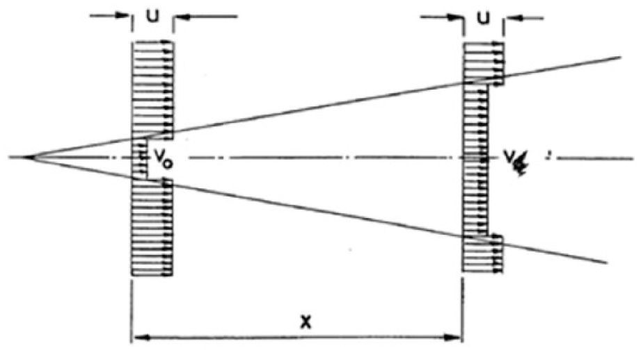
Schematic wake model (Jensen, 1983).

In WindSim, the wakes from multiple wind turbines have been combined using a linear superposition of the wake deficits by equating the sum of the kinetic energy deficits of each wake (Meissner, 2015), while openWind considers the largest deficit wake combination approach (AWS Truepower, 2010).

Model setup

Basic flow calculations

The input of a terrain description as a digital elevation model (DEM) is necessary to initialize microscale models used for wind energy applications. A wind climatology, that is, a statistical description of the wind speed and direction observed in the domain area, is necessary before starting mass-conserving models (according to the formulation of the previous section), but, for CFD, it is used only to adjust the simulated wind field as a post-processing.

The same DEM was used as the input to both models. Its area extends along 20 km × 20 km in horizontal dimensions. The terrain is hypothetic, perfectly flat, with an also idealized uniform roughness length, herein defined equal to 0.04 m, typical of cropland/pasture areas. The computational grid was set with a horizontal resolution of 100 m.

One wind climatology was positioned at the central point of the domain. The dataset has been physically obtained from a meteorological mast (“met mast”) at 80 m above ground level (agl) during 3.5 years. These sampling data showed very predominant Easterly winds (Figure 2). The geographical identity of this site is irrelevant, since the wind data were employed generically only to force the models on adjusting the simulated wind fields.

Figure 2.

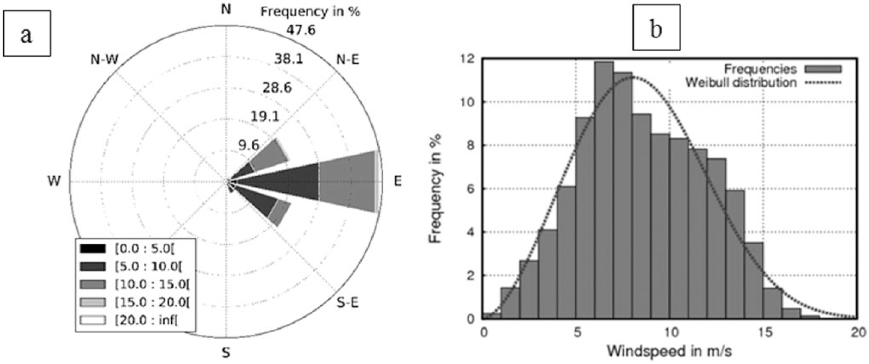
Directional wind rose (a) and frequency distribution (b) of the wind measurements used to the flat terrain considered in this study.

The numerical and physical parameters that can be set by the user in these tools were kept equal, enabling a fair comparison. It encloses the following:

Boundary layer height—200 m;

Number of wind directions—12 sectors;

Air density—1.225 kg/m³.

Some additional configurations are to be set at the CFD tool, specifically:

Geostrophic wind speed—10 m/s;

Turbulence model—standard k–ε.

AEP calculations

For AEP estimation, additional inputs of the turbines’ characteristics are necessary, such as power and thrust coefficient curves, hub height, and rotor diameter.

The following parameters related to AEP calculation and wake effect modeling were used in both models:

Turbine model—Vestas V-90 (hub height: 80 m; rotor diameter (D): 90 m);

Wake model—“Jensen model” (“Model 1” in WindSim and “Park Model” in openWind);

Wake influence range—50D;

Subsectors for wake calculation $(n D)$ : 72 (total).

The computation of the total (gross) AEP is according to the formulation of equation (11). It is based on the wind speed frequency distribution and on the power curve of the turbine model chosen, besides being dependent on the number of turbines in a wind farm $(n T)$

A E P = 8766 \times \sum_{i = 1}^{n D} \sum_{j = 1}^{n U} \sum_{k = 1}^{n T} F_{i j k} P_{i j k}

(11)

where $n D$ is the subdivision of sectors, $n U$ is the subdivision of bins of wind speed, $F_{i j k}$ is the probability of the wind coming from the direction sector $i$ at wind speed bin $j$ at turbine $k$ , $P_{i j k}$ is the associated power (kW), and 8766 is the average number of hours in one year (AWS Truepower, 2010).

For each direction, each wind speed bin value of the climatology is transferred according to the speed-up to get the wind speed for that bin at the turbine position. In openWind, the power for a particular speed bin is then defined as,

the average power derived from the power curve over the interval of the bin limits. If no point on the user-defined power curve lies within this interval, then this is the average of the values at the two end points, which are determined by linear interpolation from the bracketing points on the curve. If the power curve contains one or more points between the limits of the bin then the averaging is done from the inferior limit to the first point, then from the first point to the second point, and so on, until the superior limit is reached. The weight given to each element in the combined average depends on the width of the corresponding speed interval. (AWS Truepower, 2010: 4)

In WindSim, the transferred wind speed value for a bin is used to find the two closest power values at the power curve and the equivalent power is obtained by linear interpolation (Meissner, personal communication, 16 November 2016).

To test the influence of wake model implementation in each computational tool, different positioning of wind turbines inside the simulation domain was tested. Configurations with one, two, and four turbines were used, equally spaced around the met mast, being spaced apart one from each other as multiple of rotor diameters: 1.5D, 2D, 3D, and 500 m. When using two turbines, they were positioned in line with the wind flow and also in crosswind (diagonal 45°) array in relation to the predominant wind direction from the East (see Figures 2 and 3). The layout with four turbines was in square array. When using only one turbine, it was located at the position of the climatology, although its position is irrelevant, as will be further discussed. One should, however, remember that this work is not intended to be compared to a wind farm project, but only a study of models.

Figure 3.

Configurations of objects’ distribution on the simulation domain, where • represents the met mast and ▲ represents the wind turbines.

Results

The first evaluation to be considered is the wind field generated by each model approach. In this stage, any turbine was included in the wind farm, but only the central met mast provided wind data in order to adjust the basic simulated wind field to the observed wind speed values and generate the so-called wind resource map. CFD models just calculate the terrain-induced speed-ups and do not take account of this adjustment. So, it was performed in a post-processing module available in WindSim.

Figure 4 shows the wind resource maps generated by both models. As could be expected for a perfectly flat terrain, both wind fields have uniform wind speed along the whole domain with no speed-ups. This is coherent since any orographic obstacle or roughness changes are present. The constant value around 8.58 m/s agrees with the mean wind speed obtained from the wind dataset. The small difference (from 8.583 to 8.585 m/s) represents 0.07% in terms of energy (the wind power density is proportional to the third power of the wind speed). Hence, for terrain-independent cases and without any thermal effect, CFD and mass-conserving techniques have been considered equivalent for simulating the basic flow.

Figure 4.

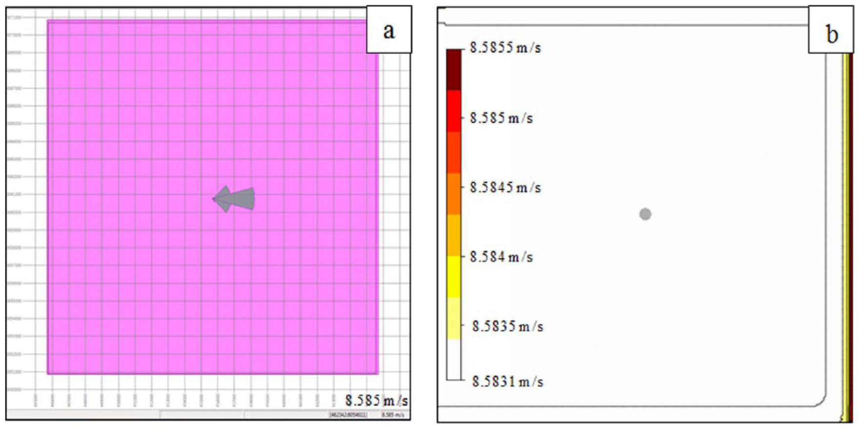
Wind resource maps at 80 m agl: (a) mass-conserving and (b) CFD.

Next, wind turbines were positioned over the simulation domain as described in the previous section to evaluate the AEP assessment.

Table 1 presents the values of gross AEP for all configurations of wind turbine distribution over the domain, as well as the comparison between the estimations obtained with the two wind flow models employed herein. It allows to compare the implementation of AEP calculation in the tools. The percentage difference (indicated as “% diff” in the tables) considers the absolute difference between the models relative to the WindSim result. The differences in AEP estimations (0.02%~0.05%) are smaller than the difference due to the wind field properly (0.07%), which means that the implementation of AEP computation in both tools provides the same results. Moreover, it was confirmed that the production is independent of the spacing, since, at this point, the interactions between turbines are not considered yet (wake effects neglected). And the total AEP is directly proportional to the number of turbines. Also for the configuration with only one turbine, since the wind field is totally uniform, the position of this turbine is irrelevant, resulting always in the same AEP.

Table 1.

Gross AEP estimated for different configurations of turbines (T) in GWh/year.

	Turbine spacing: 500 m			Turbine spacing: 3D = 270 m
	2T in line	2T diagonal	4T square	2T in line	2T diagonal	4T square
WindSim	18.781	18.781	37.562	18.781	18.781	37.562
openWind	18.790	18.790	37.579	18.790	18.790	37.579
OW–WS	0.009	0.009	0.017	0.009	0.009	0.017
% diff	0.05	0.05	0.05	0.05	0.05	0.05
	Turbine spacing: 2D = 180 m			Turbine spacing: 1.5D = 135 m
	2T in line	2T diagonal	4T square	2T in line	2T diagonal	4T square
WindSim	18.781	18.781	37.562	18.781	18.781	37.562
openWind	18.790	18.790	37.579	18.790	18.790	37.579
OW–WS	0.009	0.009	0.017	0.009	0.009	0.017
% diff	0.05	0.05	0.05	0.05	0.05	0.05
	1T	WS	OW	% diff
		9.393	9.395	0.02

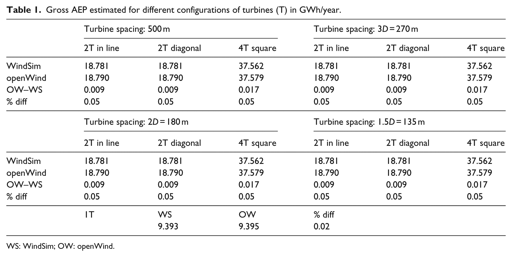
WS: WindSim; OW: openWind.

The following analyses are addressed only to the wake model implementation, since the preprocessed wind fields and gross AEP were certified to be equivalent.

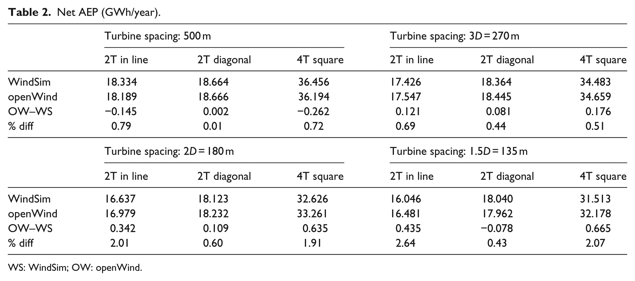
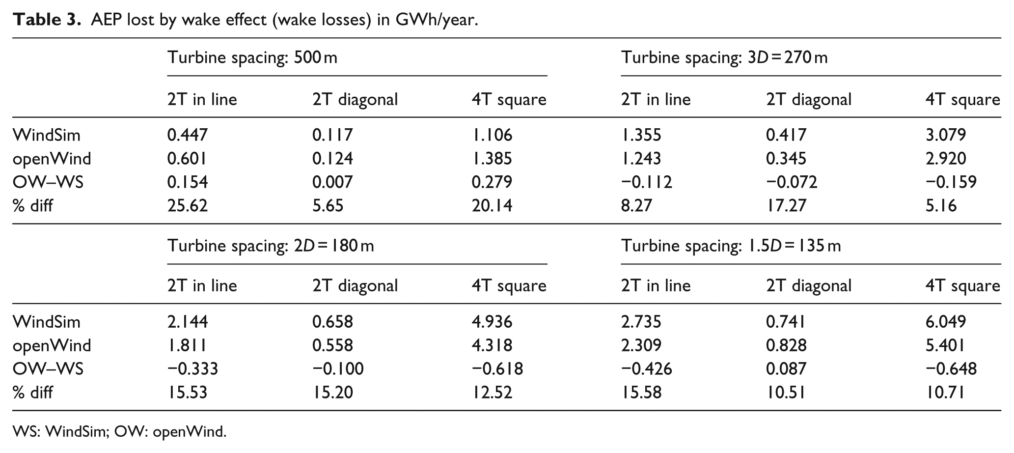
The net AEP is presented in Table 2. It discounts from the gross AEP the losses due to the wake effects that are presented in Table 3. All the tables are organized similarly, showing the different wind turbines’ positioning and spacing.

Table 2.

Net AEP (GWh/year).

	Turbine spacing: 500 m			Turbine spacing: 3D = 270 m
	2T in line	2T diagonal	4T square	2T in line	2T diagonal	4T square
WindSim	18.334	18.664	36.456	17.426	18.364	34.483
openWind	18.189	18.666	36.194	17.547	18.445	34.659
OW–WS	−0.145	0.002	−0.262	0.121	0.081	0.176
% diff	0.79	0.01	0.72	0.69	0.44	0.51
	Turbine spacing: 2D = 180 m			Turbine spacing: 1.5D = 135 m
	2T in line	2T diagonal	4T square	2T in line	2T diagonal	4T square
WindSim	16.637	18.123	32.626	16.046	18.040	31.513
openWind	16.979	18.232	33.261	16.481	17.962	32.178
OW–WS	0.342	0.109	0.635	0.435	−0.078	0.665
% diff	2.01	0.60	1.91	2.64	0.43	2.07

WS: WindSim; OW: openWind.

Table 3.

AEP lost by wake effect (wake losses) in GWh/year.

	Turbine spacing: 500 m			Turbine spacing: 3D = 270 m
	2T in line	2T diagonal	4T square	2T in line	2T diagonal	4T square
WindSim	0.447	0.117	1.106	1.355	0.417	3.079
openWind	0.601	0.124	1.385	1.243	0.345	2.920
OW–WS	0.154	0.007	0.279	−0.112	−0.072	−0.159
% diff	25.62	5.65	20.14	8.27	17.27	5.16
	Turbine spacing: 2D = 180 m			Turbine spacing: 1.5D = 135 m
	2T in line	2T diagonal	4T square	2T in line	2T diagonal	4T square
WindSim	2.144	0.658	4.936	2.735	0.741	6.049
openWind	1.811	0.558	4.318	2.309	0.828	5.401
OW–WS	−0.333	−0.100	−0.618	−0.426	0.087	−0.648
% diff	15.53	15.20	12.52	15.58	10.51	10.71

WS: WindSim; OW: openWind.

Comparisons of all turbine arrays showed that the differences found between the net AEP estimated by each of the two models were small, not higher than 2.6%.

The smallest differences were observed with the arrangement with two turbines in a crosswind array, not more than 0.6% in net AEP. In this layout, the wake effect between the turbines was very small due to the fact that the most predominant wind direction is from the East. Although the flow is disturbed when passing through the upstream turbine rotor, the kinetic energy deficit is weakly felt by the other turbine located more to the North. The differences observed in the net AEP for a single wake layout (two wind turbine arrays) are due solely to wake model implementation. There is not any effect of approach to wake combination in these two wind turbine arrays.

The highest differences were seen when turbines were arranged in line along the main wind direction (both with two or four turbines). The maximum difference of 2.6% between the models has occurred in these cases. In these layouts, the disturbed flow reaches the downstream turbine rotors with a more significant kinetic energy deficit, since they are right behind the shadow of the wakes, affecting their production.

Table 3 allows confirming that the smaller the turbine spacing, the larger the wake losses. Since the velocity deficit is inversely proportional to the downstream distance from the rotor (equation (10)), the closer the wind turbines are, the less is the recovery of the kinetic energy lost by the flow (absorbed by the upstream turbine), when reaching the next turbine. The maximum relative difference verified in the wake effect evaluation between the different tools was 25.62% and the minimum was 5.16%.

From the tables, one can also observe that, in absolute values, the smaller the turbine spacing, the larger the difference between the estimations from the models. Following the abovementioned theory, this means that the net AEP results were sensitive to the wake model implementation in each approach. The wake losses calculated by WindSim were higher than those calculated by openWind, except for the largest spacing (500 m). The maximum difference was in the order of 6.5 × 10^–1 GWh/year, which represents approximately 2%. This value is higher than 0.07% that was due to the small differences in the wind fields. In a quantitative example, if we consider 6.5 × 10^–1 GWh along 20 years of wind farm life span and a contract of R$203.46 per MWh (approximately US$63.50), based on the price of the wind energy sold in the last Brazilian energy auction, this means a difference of R$2.6 million (or ~US$830,000) in the project.

Under the conditions considered in the simulations, it can be concluded that there is a difference in the wake model implementation. Furthermore, one can infer that, in simulations over non-flat terrains, the differences higher than approximately 2% in the values of net AEP (i.e. considering wake losses) are attributed to the capacity of each method/code to reproduce the behavior of the wind over each topography.

Conclusion

In this study, AEP assessments from two different tools for wind resource evaluation have been compared to analyze the power curve and a wake model implementation. To avoid the effect of different wind flow modeling in these computational tools, this study was carried out for different layouts of wind turbines distributed over a perfectly flat terrain with uniform surface roughness.

The analysis conducted showed that, in the absence of topographic perturbations and thermal phenomena, the mass-conserving and CFD approaches are compatible on the wind field modeling.

When the wake effects were disregarded, the differences between the gross AEP implementation in the tools were negligible (0.05%), smaller than 0.07% due to the small differences in the wind fields. However, when the wake effects were considered, the comparison of the net AEP results showed sensitivity face to the same wake model implementation, with differences of up to 2.6% between the results of these two computational tools. The wake losses calculated by WindSim were higher than those calculated by openWind, except for the largest spacing (500 m). As the wake kinetic energy deficit is a function of the downstream distance from the upstream turbine rotor, the smaller turbine spacing resulted in larger differences between the tools’ estimations. Considering the predominance of winds from the East in the wind climatology used, the highest wake effects (and, consequently, the highest differences between tools) were found in the layouts with in line array of turbines.

This study has analyzed how two different computational tools (WindSim and openWind) evaluate the implementation of turbine power curve and a wake model, avoiding the terrain effects. The next step is Part II of the ongoing work, in which the comparison of the effect of different wind field modeling in AEP estimation will be performed using these two tools in a complex terrain where the trade winds are enhanced by thermal effects.

Footnotes

Declaration of conflicting interests

The author(s) declared no potential conflicts of interest with respect to the research, authorship, and/or publication of this article.

Funding

The author(s) received no financial support for the research, authorship, and/or publication of this article.

ORCID iD

Adaiana F Gomes da Silva

References

Albani

Ibrahim

(2014) An assessment of wind energy potential for selected sites in Malaysia using feed-in tariff criteria. Wind Engineering 38(3): 249–259.

AWS Truepower (2010) openWind: Theoretical basis and validation. Report version no. 1.3. Albany, NY: AWS Truepower.

Ayotte

(2008) Computational modelling for wind energy assessment. Journal of Wind Engineering and Industrial Aerodynamics 96: 1571–1590.

Beaucage

Brower

Tensen

(2014) Evaluation of four numerical wind flow models for wind resource mapping. Wind Energy 17(2): 197–208.

Bechmann

Sørensen

Berg

et al . (2011) The Bolund experiment, part II: Blind comparison of microscale flow models. Boundary-Layer Meteorology 141(2): 245–271.

Bengtsson

(2015) Turbulence wind flow modeling in complex terrain. MSc Dissertation, Chalmers University of Technology, Gothenburg.

Berge

Gravdahl

Schelling

et al . (2006) Wind in complex terrain: A comparison of WAsP and two CFD-models. In: Proceedings of the European wind energy conference and exhibition, 27 February–2 March, Athens.

Bitsuamlak

Stathopoulos

Asce

et al . (2004) Numerical evaluation of wind flow over complex terrain: Review. Journal of Aerospace Engineering 17(4): 135–145.

Blocken

Hout

Dekker

et al . (2015) CFD simulation of wind flow over natural complex terrain: Case study with validation by field measurements for Ria de Ferrol, Galicia, Spain. Journal of Wind Engineering and Industrial Aerodynamics 147: 43–57.

10.

Brower

(1999) Validation of the WindMap program and development of MesoMap. In: Proceedings of the American wind energy association windpower conference, Washington, DC.

11.

Castellani

Astolfi

Burlando

et al . (2015) Numerical modelling for wind farm operational assessment in complex terrain. Journal of Wind Engineering and Industrial Aerodynamics 147: 320–329.

12.

Cataldo

Zeballos

(2009) Roughness terrain consideration in a wind interpolation numerical model. In: Proceedings of the 11th Americas conference on wind engineering, San Juan, 22–26 June, p. 12. Kanagawa, Japan: IAWE.

13.

Eriksson

(2013) A mass conserving wind model evaluation with finite element. MSc Dissertation, Umeå University, Umeå.

14.

Gasset

Landry

Gagnon

(2012) A comparison of wind flow models for wind resource assessment in wind energy applications. Energies 5(11): 4288–4322.

15.

González

Payán

Santos

JMR

et al . (2014) A review and recent developments in the optimal wind-turbine micro-siting problem. Renewable and Sustainable Energy Reviews 30: 133–144.

16.

Gravdahl

(1998) Meso scale modeling with a Reynolds averaged Navier-Stokes Solver: Assessment of wind resources along the Norwegian coast. In: Proceedings of the 31st IEA experts meeting, Roskilde, pp. 31–45. Tønsberg: WindSim AS.

17.

Jafari

Chokani

Abhari

(2012) An immersed boundary method for simulation of wind flow over complex terrain. Journal of Solar Energy Engineering 134(1): 011006.

18.

Jensen

(1983) A note on wind generator interaction. Report no. Risø-M-2411, Roskilde: Risø National Laboratory.

19.

Katíc

Højstrup

Jensen

(1986) A simple model for cluster efficiency. In: Proceedings of the European wind energy conference and exhibition, Rome, 7–9 October.

20.

Kumar

Ringenberg

Depuru

et al . (2016) Wind energy: Trends and enabling technologies. Renewable and Sustainable Energy Reviews 53: 209–224.

21.

Meissner

(2015) WindSim Getting Started: WindSim 7 (8th edn). Tønsberg: WindSim AS.

22.

Neophytou

Gowardhan

Brown

(2011) An inter-comparison of three urban wind models using Oklahoma City Joint Urban 2003 wind field measurements. Journal of Wind Engineering and Industrial Aerodynamics 99(4): 357–368.

23.

Phillips

Traci

(1979) A preliminary user’s guide for the NOABL objective analysis code. Report no. DOE/ET/20280-T1, La Jolla, CA: U.S. Department of Energy.

24.

Prospathopoulos

Politis

Chaviaropoulos

(2012) Application of a 3D RANS solver on the complex hill of Bolund and assessment of the wind flow predictions. Journal of Wind Engineering and Industrial Aerodynamics 107–108: 149–159.

25.

Ramechecandane

Gravdahl

(2012) Numerical investigations on wind flow over complex terrain. Wind Engineering 36(3): 273–296.

26.

Rasouli

Hangan

(2013) Microscale computational fluid dynamics simulation for wind mapping over complex topographic terrains. Journal of Solar Energy Engineering 135(4): 041005.

27.

Rodrigo

(2010) State-of-the-art of wind resource assessment. Report version no. 3. Sarriguren: WAUDIT; CENER.

28.

Seim

(2015) Validating kinematic wake models in complex terrain using CFD. MSc Dissertation, Norwegian University of Life Sciences, Ås, Akershus.

29.

Shakoor

Hassan

Raheem

et al . (2016) Wake effect modeling: A review of wind farm layout optimization using Jensen’s model. Renewable and Sustainable Energy Reviews 58: 1048–1059.

30.

Sherman

(1978) A mass-consistent model for wind fields over complex terrain. Journal of Applied Meteorology 17: 312–319.

31.

Simões

Estanqueiro

(2016) A new methodology for urban wind resource assessment. Renewable Energy 89: 598–605.

32.

Sumner

Watters

Masson

(2010) CFD in wind energy: The virtual, multiscale wind tunnel. Energies 3: 989–1013.

33.

Theodoropoulos

Deligiorgis

(2009) WindSim CFD model validation in a mixed coastal & mountainous region with complex terrain. In: Proceedings of the European wind energy conference and exhibition, Vol. 6, Marseille, 16–19 March, pp. 3909–3918. Markopoulo Mesogaias: ISTOS RENEWABLES.

34.

Timander

Westerlund

(2012) Reliability of wind farm design tools in complex terrain: A comparative study of commercial software. MSc Dissertation, KTH School of Industrial Engineering and Management, Stockholm.

35.

Versteeg

HKE

Malalasekera

(2007) An Introduction to Computational Fluid Dynamics: The Finite Volume Method (2nd edn). Harlow: Pearson Education.

36.

Wakes

Maegli

Dickinson

et al . (2010) Numerical modelling of wind flow over a complex topography. Environmental Modelling & Software 25(2): 237–247.

37.

Walmsley

Troen

Lalas

et al . (1990) Surface-layer flow in complex terrain: Comparison of models and full-scale observations. Boundary-Layer Meteorology 52: 259–281.