Improved regularized extreme learning machine short-term wind speed prediction based on gray correlation analysis

Abstract

Accurate wind speed prediction is of great significance to the stable operation of the power grid when large-scale wind power is connected to the grid. This article proposes a new multi-step wind speed combination prediction model based on gray correlation analysis. First, the gray correlation analysis is performed on wind speed–related attributes, the more relevant attribute factors are selected as the input set of the prediction model, and the regularized extreme learning machine improved by the cuckoo optimization algorithm is used to perform multi-step prediction of wind speed. Then, an error self-tuning model is established to further improve the prediction accuracy. Finally, the measured results of different wind farms and seasons are selected to simulate the prediction effect of the proposed model, and the prediction accuracy and generalization ability of the proposed model are verified through comparative analysis.

Keywords

Wind speed prediction gray correlation analysis regularized extreme learning machine cuckoo optimization algorithm error self-tuning mode

Introduction

Wind speed prediction of wind farms can improve the dispatching economy of grids with renewable energy sources and the operational safety of wind farms (Liu and Dong, 2016; Pan et al., 2019), but the characteristics of wind speed fluctuation, indirectness, and low energy density will also reduce power systems’ reliability of operation (Yang et al., 2018). Therefore, accurate wind speed prediction becomes more and more important for wind power grid connection and the operation of power systems (Zhang et al., 2018).

Existing wind speed prediction methods include physical methods (Feng et al., 2011,), mathematical methods (Yang et al., 2017), and artificial intelligence methods (Wang et al., 2018; Zhang et al., 2017). At present, most scholars around the world pay more attention to wind speed prediction methods based on artificial intelligence. Among them, the parameter setting of the extreme learning machine (ELM) is simple, the learning ability is strong, the calculation speed is fast, and it is easy to converge (Li and Li, 2016; Ye et al., 2017). But its interlayer weights and offsets are generated randomly, which has a greater impact on the prediction effect. Wang et al. (2015b) used the cuckoo optimization algorithm (COA) to optimize the parameters of the support vector machine (SVM). The results show that COA can effectively improve the accuracy of the prediction model. Xiang et al. (2019) analyzed a variety of wind speed hybrid prediction models and found that the ELM can obtain better prediction results in both single-step and multi-step prediction. Zhu et al. (2017) improved the accuracy of the ultra-short-term wind power prediction model by analyzing the correlation between various attribute factors and wind power and taking attribute factors as one of the considerations for wind power modeling. In Yang et al. (2017), the relationship between wind speed and power was analyzed using gray relational decision-making, and a wind power prediction model was established using the gray relational relationship and the wind speed–power curve.

This article proposes a new wind speed prediction model based on gray relational analysis (GRA) and an improved regularized extreme learning machine (RELM). Based on the gray correlation theory, the correlation between various attribute factors and wind speed are calculated. In order to reduce the complexity of the model, the multi-attribute time series is selected to reduce the input data. The COA was used to optimize the parameters of RELM in order to construct a combined wind speed prediction model. The obtained prediction results are corrected through error self-tuning mode to reduce prediction errors and obtain more accurate prediction results. Finally, the prediction results are compared with the actual wind farm data to verify the effectiveness of the proposed model.

Attribute optimization based on gray correlation analysis

GRA

Gray system analysis judges the correlation by determining the geometric similarity between the reference data column and the comparative data column (Zhang et al., 2011). The wind speed reference sequence is

S_{0} = [s_{0} (1), \dots, s_{0} (t), \dots, s_{0} (n)]

(1)

where s₀(t) represents the measured wind speed value at time t in the reference sequence and n is the total number of time points.

The comparison sequence S_ij is

S_{ij} = [s_{ij} (1), \dots, s_{ij} (t), \dots, s_{ij} (n)]

(2)

The specific steps are as follows:

1. Initialize each sequence

S'_{ij} = \frac{S_{ij}}{s_{ij} (1)} = [{s'}_{ij} (1), \dots, {s'}_{ij} (t), \dots, {s'}_{ij} (n)]

(3)

2. Find the absolute value sequence of the difference between the reference sequence and the initial value of the comparison sequence as

Δ_{i} (t) = | {s'}_{0} (t) - {s'}_{ij} (t) |

(4)

3. Calculate the correlation coefficient to characterize the correlation between two groups of sequences

γ [s_{0} (t), s_{ij} (t)] = \frac{min_{ij} min_{t} Δ_{ij} (t) + κ max_{ij} max_{t} Δ_{ij} (t)}{Δ_{ij} (t) + κ max_{ij} max_{t} Δ_{ij} (t)}

(5)

where $min_{ij} min_{t} Δ_{ij} (t)$ and $max_{ij} max_{t} Δ_{ij} (t)$ are the minimum and maximum values of the sequence Δ(t) at different times, respectively, and κ is the resolution coefficient, where κ∈ (0,1) with a smaller κ indicating a higher resolution.

Define the time series correlation coefficient to characterize its correlation degree

γ (S_{0}, S_{ij}) = \frac{1}{n} \sum_{t = 1}^{n} γ [s_{0} (t), s_{ij} (t)]

(6)

Through the above steps, the wind speed sequence and the attribute sequence data are quantified and analyzed to obtain the characteristic coefficient of the target S₀.

Analysis of related attribute selection

Taking the measured data and related meteorological data of a wind farm in the Northeast as an example to conduct the correlation analysis, the typical monthly original wind speed sequence for each quarter is shown in Figure 1.

Figure 1.

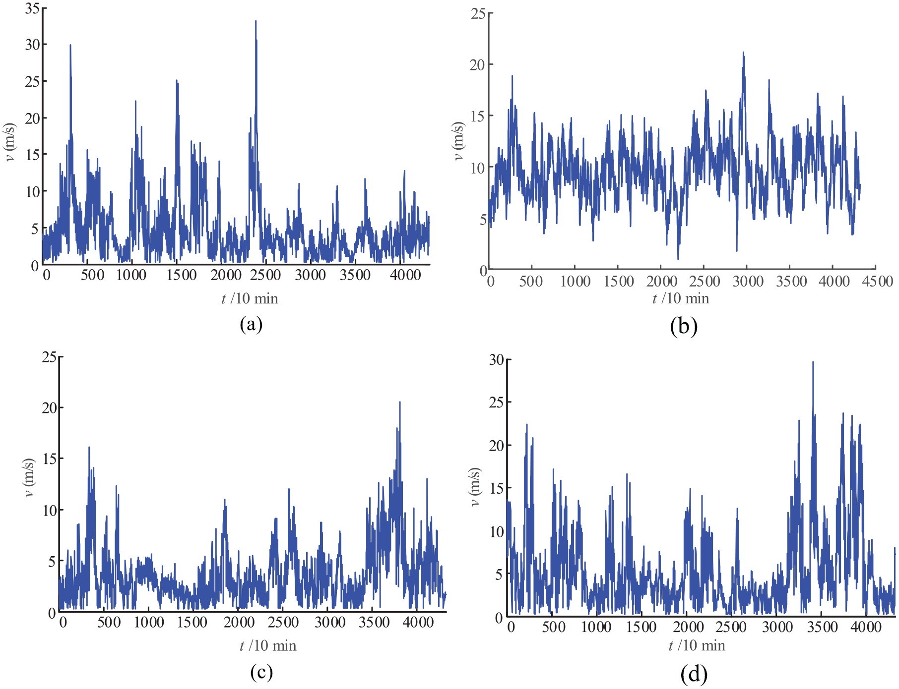
Original wind speed sequence of the northeast wind farm: (a) typical spring month—April; (b) typical summer month—July; (c) typical autumn month—October; and (d) typical winter month—November.

It can be seen from Figure 1 that winter has the most severe fluctuations and the wind speed difference is large at different times. However, the fluctuation of wind speed in spring is more regular, which increases or decreases periodically. The changes of wind speed in summer and autumn are similar and the fluctuation is relatively flat. Because wind power is generated by wind speed, there is a certain similarity between the fluctuations of the two. In this article, wind power fluctuations in different seasons are selected as an attribute factor to train the prediction model.

There are many attributes related to wind speed, including wind power (seasonal wind power fluctuations), wind direction, temperature, standard deviation of air pressure, and air density (Wang et al., 2015a). It has been confirmed that there are obvious deficiencies in predicting future values based on historical wind speed information alone. And the model’s ability to learn random fluctuations in wind speed is poor. Therefore, this article selects the above five attribute factors for the analysis and reasonably selects the input variables of the model. The correlation analysis of each time series is performed according to the gray correlation theory, and the results are shown in Table 1.

Table 1.

Results of the correlation of various attribute factors.

Classification	Wind direction	Wind power	Temperature	Atmospheric pressure	Air density
v	0.2945	0.9513	−0.1591	0.3257	0.5781

As can be seen from Table 1, the correlation between the wind speed sequence and the wind power sequence is the highest, reaching 0.9513. The correlation degree with air density is the second highest, and the correlation coefficient is 0.5781. In addition, the correlation degree between wind speed and wind direction as well as wind speed and temperature is low, and the correlation coefficients are 0.2945 and −0.1591, respectively. Due to the special monsoon climate in the Northeast, when the temperature is high in summer, the wind speed is usually smaller than that that in spring and autumn, so it shows a negative correlation with temperature.

Attribute optimization based on the improved RELM combination prediction model

RELM

y (x) = \sum_{K = 1}^{L} β_{K} G (ω_{K} x + b_{K})

(7)

where G is the activation function, β _K is the output weight matrix, ω _K is the input weight matrix, b_K is the bias of the Kth hidden layer neuron, and L is the number of hidden layer neurons.

In order to improve the prediction accuracy of the ELM network, a regularization coefficient is introduced to minimize the structural risk.

1. Establish the objective function

{\begin{matrix} min U = min_{β} {\frac{η}{2} ‖ ξ ‖^{2} + \frac{1}{2} ‖ β ‖^{2}} \\ ξ = H β - T \end{matrix}

(8)

where η is the regularization coefficient, ||ξ||² is the empirical risk, || β ||² is the structural risk, ξ is the sum of the training set errors, H is the output layer of the hidden layer, and T is the output set.

2. Constructing Lagrange’s equation

L (α, ξ, β) = \frac{η}{2} ‖ ξ ‖^{2} + \frac{1}{2} ‖ β ‖^{2} - α (H β - T - ξ)

(9)

where α is a Lagrangian multiplier.

3. Calculate the output weight matrix

\tilde{β} = {(H^{T} H + \frac{I}{η})}^{- 1} H^{T} T

(10)

where I is the identity matrix.

4. Substituting equation (10) into equation (7), a mathematical model of wind speed prediction based on RELM can be obtained

y = \sum_{i = 1}^{L} {\tilde{β}}_{i} G (ω_{i} x + b_{i})

(11)

COA

The input-hidden interlayer weights and biases of RELM are randomly generated after the number of hidden layer neurons is determined. To avoid the randomness of parameter selection, the COA is used to optimize the input-hidden interlayer weights and biases. In order to achieve a more ideal prediction effect (Huang, 2015), the steps are as follows:

1. The population is initialized.

2. New solutions are generated by Levy flight. The new solution for each bird’s nest can be calculated as

X_{i}^{new} = X_{bes t_{i}} + λ \cdot l_{1} \cdot Δ X_{i}^{new}

(12)

Δ X_{i}^{new} = ν \frac{σ_{x} (δ)}{σ_{y} (δ)} (X_{bes t_{i}} - Q_{best})

(13)

where $X_{bes t_{i}}$ is the individual optimal solution, G_best is the population optimal solution, λ > 0 is the iterative step size, and l₁ is a random number uniformly distributed between 0 and 1. The variable v is defined as l_x/l_y, where l_x and l_y are normally distributed random numbers with σ_x(δ) and σ_y(δ) being their standard deviations, respectively.

3. Find the strange egg and randomize the bird’s nest. Assume that the probability that the mother will find a strange egg in the nest is P_a. When a strange egg is discovered, a new solution will be generated as follows

X_{i}^{dis} = X_{bes t_{i}} + R Δ X_{i}^{dis}

(14)

Δ X_{i}^{dis} = l_{2} [l_{p 1} (X_{bes t_{i}}) - l_{p 2} (X_{bes t_{i}})]

(15)

where l₂ is a random number uniformly distributed between 0 and 1. l_p₁ and l_p₂ are random perturbations when the optimal solution of the bird’s nest is $Y_{bes t_{i}}$ . The parameter R is determined by the formula

R = {\begin{matrix} 1, l_{2} < P_{a} \\ 0, l_{2} \geq P_{a} \end{matrix}

(16)

4. When the maximum number of iterations is reached, the algorithm ends.

Compared with optimization algorithms such as particle swarm optimization, the COA has the advantages of high accuracy and fast convergence. In this article, the absolute average error of six single-step predictions is used as the fitness function of COA. The parameter optimization training of RELM is performed to construct a multi-step wind speed prediction combination model. For short-term prediction, historical wind speed data and Numerical Weather Prediction (NWP) data are selected as training data, and C-C method (Letellier, 2017) is used to reconstruct phase space of historical time series.

Model self-tuning algorithm

Based on the COA-RELM model, in order to further reduce the model prediction error and improve the prediction accuracy of the combined model, this article adds error self-tuning. At present, most of the error correlation linear analysis methods are selected to reduce the prediction error (Tang et al., 2019). The combined forecasting model is modified by solving the functional relationship between the historical forecasting error and the input. In this article, the mean absolute percentage error (MAPE) is selected as the self-tuning standard

ε_{M} = f (x_{1}, \dots, x_{n}) = k_{1} x_{1} + k_{2} x_{2} + \dots + k_{n} x_{n}

(17)

where ε_M is the MAPE representing COA-RELM and f(x₁, …, x_n) is a linear function about the input (x₁, …, x_n represent the input wind speed data). The term coefficient k is obtained by the least-squares method.

The combined prediction model obtained after error self-tuning is as follows

Y = y (x_{1}, \dots, x_{n}) + f (x_{1}, \dots, x_{n})

(18)

where y(x₁, …, x_n) is the COA-RELM prediction model and Y is the final prediction result. Experiments show that the error value of the prediction model after error self-tuning is lower and the prediction effect is better.

Combined wind speed prediction model

Data processing

In order to avoid the influence of different attribute dimensions on the prediction effect, the data in the input COA-RELM are normalized as follows (Pan et al., 2018)

x' = \frac{x - min {x}}{max {x} - min {x}}

(19)

where max{x} and min{x} are the maximum and minimum values of the original data x, respectively.

The predicted value output by COA-RELM is subjected to the following inverse normalization processing, and then an error self-check is performed to calculate the error value

y = \frac{y' (max {y} - min {y}) + (min {y} + max {y})}{2}

(20)

Prediction model process

The specific flow of the combined wind speed prediction model proposed in this article is shown in Figure 2.

Figure 2.

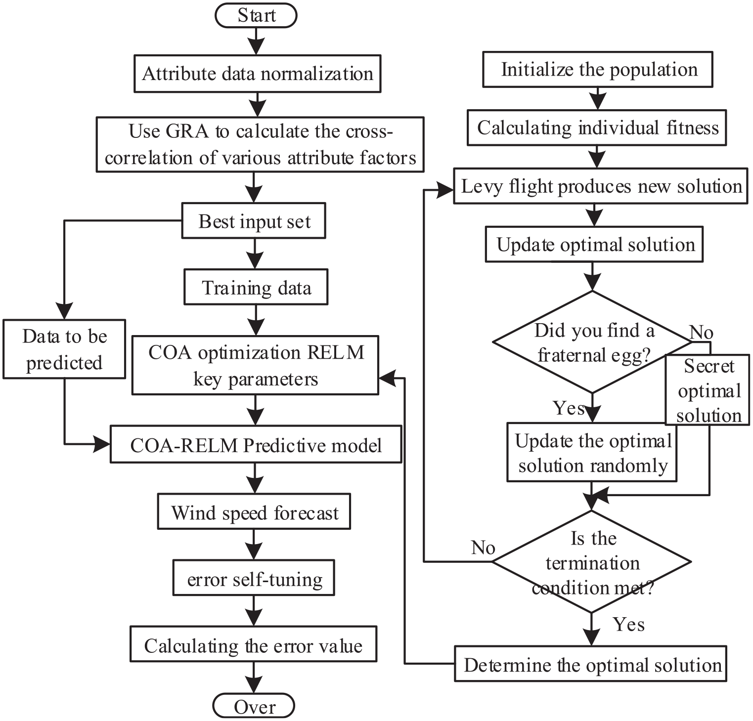
Flowchart of the combination model.

Evaluation index

In order to verify the effectiveness of the proposed model, the following two evaluation indicators are selected to evaluate the prediction results

ε_{R} = \sqrt{\frac{1}{N} \sum_{t = 1}^{N} {(x_{t} - Y_{t})}^{2}}

(21)

ε_{M} = \frac{1}{N} \sum_{t = 1}^{N} \frac{| x_{t} - Y_{t} |}{| x_{t} |} \times 100 %

(22)

where Y_t is the predicted value at time t, x_t is the actual value at time t, and N is the total number of time points in the prediction set.

Simulation analysis

The actual wind farm in the northeast region, and the actual monthly wind speed data and relevant attribute factors of the typical month of the wind farm in each quarter of 2019 are selected for the simulation analysis. The sampling interval of the original data every month is 10 min, a total of 4320 points, the data for the first 20 days are taken as the training set, the data for July 21–25 are the test set, and the data for July 26–30 are inspection set (used to check whether the model parameter settings are appropriate).

Analysis of RELM forecast results

Each attribute factor is screened based on GRA, and power, wind direction, and atmospheric pressure are selected as inputs to the model based on the results. Based on this, a rolling prediction model of 1–6 steps is established to predict the wind speed of the wind farm.

Three algorithms, namely, ELM, back propagation (BP) neural network, and SVM, were selected to perform a single-step rolling prediction of the wind speed on July 21 in the prediction set to verify the effectiveness of the method in this article (Figure 3). The training and test sets in this article were run in the MATLAB 2016b environment using Intel Core^™ i5-8500, CPU@3.00 GHz, microcomputer platform with 8.00 GB RAM.

Figure 3.

Comparison of single-step prediction results of different methods.

Each model provides a better prediction effect when the wind speed fluctuates gently. However, when the wind speed fluctuates sharply, ELM and SVM have a weak learning ability for non-linear sequences and are easy to overfit. BP has a weak learning ability for the randomness of wind speed sequences, which leads to a large deviation between the prediction result and the actual value. It has a good fitting effect on the random fluctuation of wind speed.

Analysis of prediction results of comparative models

In order to verify the accuracy of the combination model proposed in this article, different combination models were selected for rolling prediction of wind speed on the 25th of July. Among them, method 1 is COA + RELM + e (error self-tuning mode), method 2 is RELM + e, and method 3 is RELM. The results are shown in Figures 4 and 5.

Figure 4.

Single-step prediction results.

Figure 5.

Comparison of multi-step prediction results of different methods: (a) two-step prediction, (b) three-step prediction, (c) five-step prediction, and (d) six-step prediction.

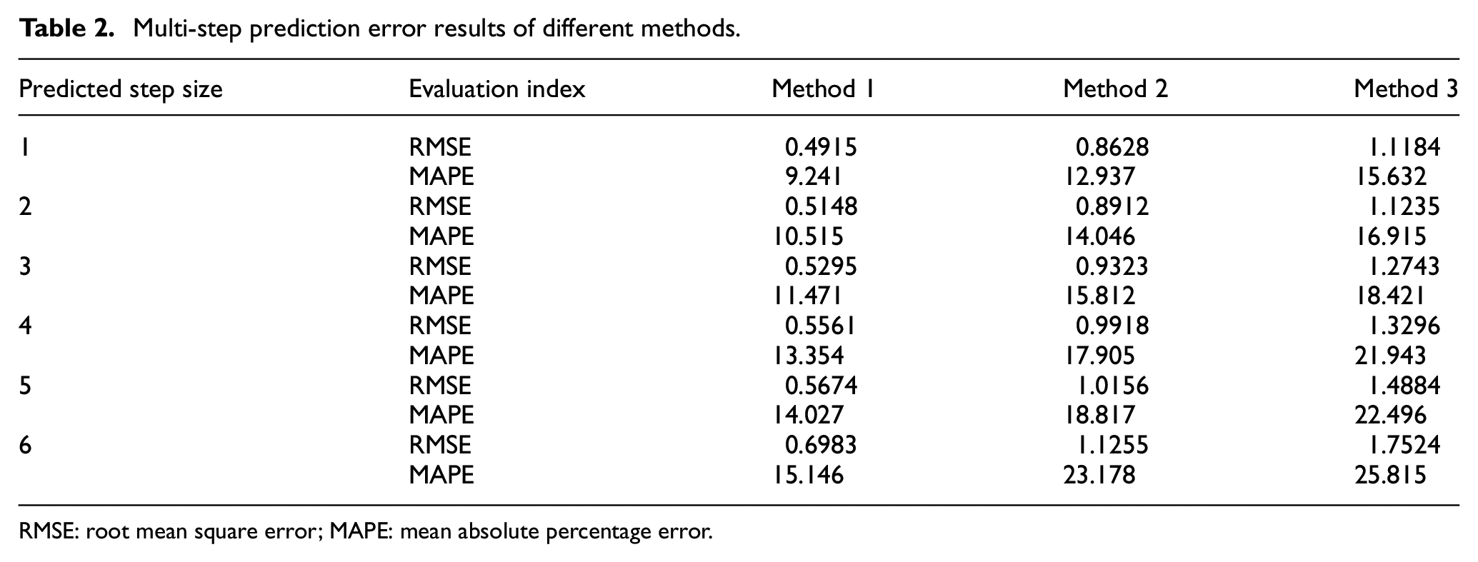
It can be seen from Figures 4 and 5 that method 1 can provide a good effect in the prediction of different step sizes, and the prediction advantage is obvious. As the step size increases, the forecasting trend is still consistent with the single-step forecasting with small changes. It has a good multi-step forecasting effect. With methods 2 and 3, as the prediction step size increases, the deviation between the prediction result and the measured data increases significantly. The specific error calculation results are shown in Table 2.

Table 2.

Multi-step prediction error results of different methods.

Predicted step size	Evaluation index	Method 1	Method 2	Method 3
1	RMSE	0.4915	0.8628	1.1184
	MAPE	9.241	12.937	15.632
2	RMSE	0.5148	0.8912	1.1235
	MAPE	10.515	14.046	16.915
3	RMSE	0.5295	0.9323	1.2743
	MAPE	11.471	15.812	18.421
4	RMSE	0.5561	0.9918	1.3296
	MAPE	13.354	17.905	21.943
5	RMSE	0.5674	1.0156	1.4884
	MAPE	14.027	18.817	22.496
6	RMSE	0.6983	1.1255	1.7524
	MAPE	15.146	23.178	25.815

RMSE: root mean square error; MAPE: mean absolute percentage error.

It can be seen from Table 2 that, in the multi-step prediction with different step sizes, the error of method 1 is smaller than that of the comparison method. Because method 2 does not optimize the RELM parameters, the prediction model’s generalization ability to different wind speed fluctuations declined. The smaller error of method 2 compared to method 3 is because method 3 does not perform self-tuning of the preliminary prediction results, thus resulting in a decrease in prediction accuracy. It is not difficult to observe certain error accumulation in the prediction results of each method. In the one-step to six-step prediction of method 1, the root mean square error (RMSE) increased by 5.505%, while that for method 2 increased by 8.681%, indicating that the optimization of the RELM parameters by COA can effectively improve the prediction accuracy and fitting effect of the model. The RMSE in method 3 at step 1 is 2.695%, which is higher compared to method 2. And the RMSE increased 2.637% in the six-step prediction. However, the effect of the error checking ability is not affected by step size, which verifies the applicability of the error self-tuning model in multi-step prediction.

In order to further verify the prediction effectiveness of the method in this article, single-step rolling prediction results are selected for typical months of the wind field in other seasons as shown in Figures 6 to 8.

Figure 6.

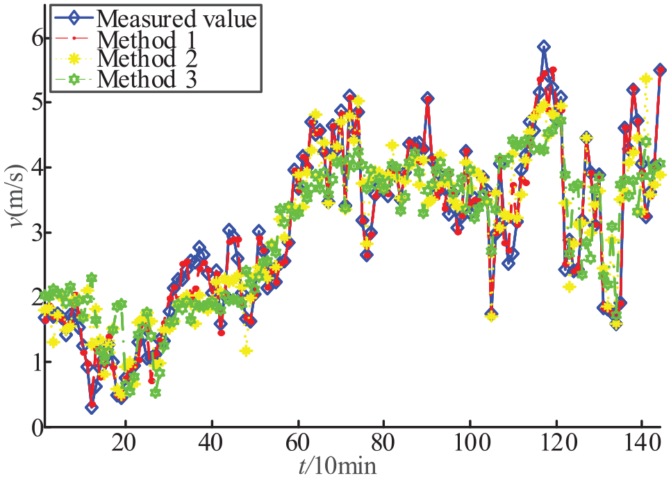
Spring (April) single-step prediction results.

Figure 7.

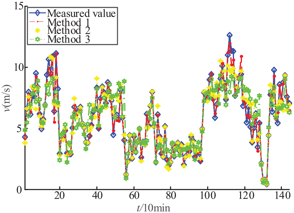
Autumn (October) single-step prediction results.

Figure 8.

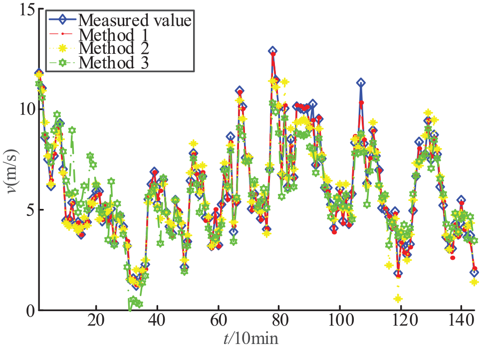
Winter (November) single-step prediction results.

It can be seen from Figures 6 to 8 that the prediction effect of method 1 in each season is better than those of methods 2 and 3, which proves the effectiveness of parameter optimization and error self-tuning models. Among them, when the wind speed in spring (April) is large and regular fluctuations, the prediction performance of the method without error self-tuning is significantly weaker than the method 1 and method 2 that pass the error check, indicating that the verified model has a stronger non-linear expression ability, can effectively reduce the generalization error. Compared with method 1, because method 2 does not optimize the parameters, although it can predict the change trend of wind speed very well, it is easy to appear in the details (such as between 110 and 120 in autumn and 105 and 110 in winter). The combination phenomenon leads to a large deviation of the predicted results from the measured data.

Error self-tuning

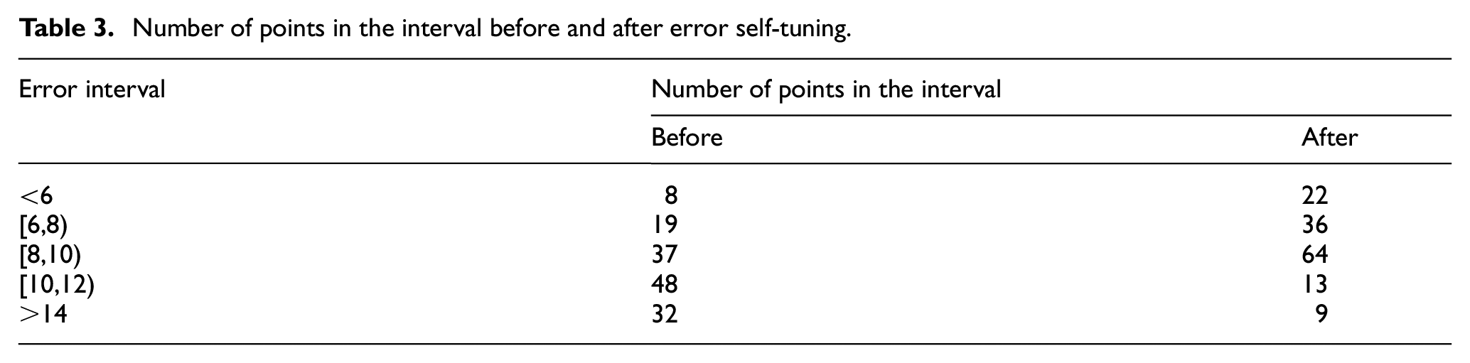
To further illustrate the effectiveness of error self-tuning, the MAPEs of the single-step prediction results before and after verification are selected for comparison. The selection results are shown in Table 3. It can be seen from Table 3 that, after verification, the number of points in the interval [10,12) is significantly reduced. Most of the points are concentrated in the interval [8,10). Statistics of 10 single-step prediction results show that the average absolute percentage error of the prediction model after verification is reduced by about 39.7% compared with the previous one. The analysis results show that the error self-tuning mode can effectively reduce the model prediction error and improve the prediction accuracy.

Table 3.

Number of points in the interval before and after error self-tuning.

Error interval	Number of points in the interval
Error interval	Before	After
<6	8	22
[6,8)	19	36
[8,10)	37	64
[10,12)	48	13
>14	32	9

Generalized verification analysis

In order to avoid the influence of the latitude, longitude, and climate of the selected area, combined with the data provided by a wind farm in Yunnan, China, the applicability of the model proposed in this article is further verified. Taking the historical wind speed data and various attribute data in January 2010 as an example, the data sampling interval is 10 min (Figure 9).

Figure 9.

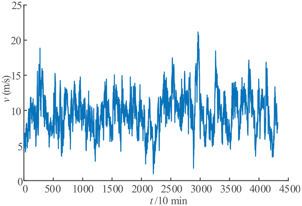
Schematic diagram of wind speed.

The wind farm is affected by geographical location and climatic environment, and the wind speed fluctuation characteristics in different quarters are quite different from those in northeast China. Correlation of each attribute sequence was calculated based on the locally measured historical meteorological data. The results are shown in Table 4. The model parameters and input set of RELM were revised, and this method is used to construct a combined model to predict wind speed. Among them, the prediction results by one-step prediction and six-step prediction are shown in Figure 10.

Table 4.

Results of the correlation of various attribute factors.

Classification	Wind direction	Wind power	Temperature	Atmospheric pressure	Air density
v	−0.0197	0.9487	0.3175	0.4316	−0.2903

Table 5.

Multi-step prediction evaluation index.

Predicted step size	Evaluation index	Method 1	Method 2	Method 3
1	RMSE	0.4334	0.7632	0.9073
1	MAPE	8.221	11.332	13.531
2	RMSE	0.4903	0.8301	1.0224
2	MAPE	9.347	12.946	15.714
3	RMSE	0.5164	0.9028	1.1622
3	MAPE	11.533	14.015	16.410
4	RMSE	0.5201	0.9434	1.2758
4	MAPE	12.724	15.903	19.275
5	RMSE	0.5437	0.9856	1.3572
5	MAPE	13.015	16.758	21.752
6	RMSE	0.5983	1.0257	1.5718
6	MAPE	13.847	21.753	23.453

RMSE: root mean square error; MAPE: mean absolute percentage error.

Figure 10.

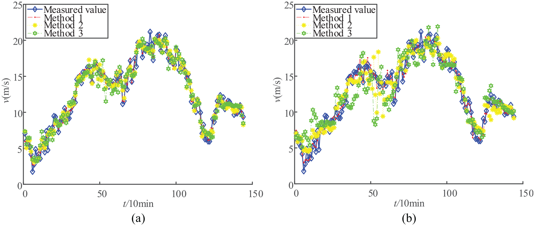
Multi-step prediction wind speed results: (a) one-step prediction and (b) six-step prediction.

From the data shown in Figure 10 and Table 4, it can be seen that the prediction results of method 1 can more accurately reflect the trend of wind speed changes, and each forecast index meets the standard requirements, which proves that the method has strong applicability and generalization ability.

Conclusion

Based on the attribute correlation degree of wind speed, a combined forecasting model is proposed to perform multi-step rolling prediction of the actual wind farm, and the following conclusions are drawn:

Analyze each wind speed attribute sequence based on gray correlation, select attribute factors with high correlation with wind speed, remove redundant information with low correlation, and improve prediction accuracy under the premise of ensuring computational efficiency.

RELM based on parameter optimization can reduce the randomness of model parameters and improve prediction performance. Combined with the wind speed fluctuations in different regions and seasons, the wind speed prediction model that conforms to the actual fluctuation conditions can be constructed through parameter modification, which has good prediction accuracy and generalization ability.

The error self-tuning model selected in this article can effectively reduce the model prediction error and is not affected by the increase in step size, thereby verifying the validity and applicability of the model proposed in this article.

Footnotes

Declaration of conflicting interests

The author(s) declared no potential conflicts of interest with respect to the research, authorship, and/or publication of this article.

Funding

The author(s) received no financial support for the research, authorship, and/or publication of this article.

ORCID iD

Wang Yue

References

Feng

Wang

Liu

, et al. (2011) Short term wind speed prediction based on physical principle. Acta Energiae Solaris Sinica 32(5): 611–616.

Huang

(2015) What are extreme learning machines? Filling the gap between Frank Rosenblatt’s Dream and John von Neumann’s puzzle. Cognitive Computation 7(3): 263–278.

Letellier

Maquet

Lesceller

, et al. (2017) On the non-eq23 of observables in phase-space reconstructions from recorded time series. Journal of Physics A: Mathematical and General 31(39): 7913–7927.

(2016) Short-term wind power prediction based on CEEMDAN-FE-KELM method. Information and Control 45(2): 11–17.

Liu

Dong

(2016) Ultra-short-term dynamic selection linear combination prediction of wind speed and wind power. Chinese Journal of Solar Energy 37(4): 1009–1016.

Pan

Benshuang

Yao

, et al. (2018) RELM wind speed prediction based on optimized FCM clustering. Power System Technology 42(3): 842–848.

Pan

Qin

Cai

, et al. (2019) A new modular wind speed prediction method. Chinese Journal of Solar Energy 40(8): 2196–2204.

Tang

Zhao

Cao

, et al. (2019) Ultra-short-term wind direction prediction based on SWLSTM algorithm. Chinese Journal of Electrical Engineering 39(15): xx.

Wang

, et al. (2018) Research on wind speed prediction based on hybrid gray theory. Chinese Journal of Solar Energy 39(12): 3544–3549.

10.

Wang

Jiang

(2015a) The study and application of a novel hybrid forecasting model—A case study of wind speed forecasting in China. Applied Energy 143: 472–488.

11.

Wang

Zhou

Jiang

, et al. (2015b) Short-term wind speed forecasting using support vector regression optimized by cuckoo optimization algorithm. Mathematical Problems in Engineering 2015(1): 1–13.

12.

Xiang

Deng

Zhao

(2019) Multi-step wind speed prediction model based on LPF-VMD and KELM. Power System Technology 43(12): 4461–4467.

13.

Yang

Chen

Huang

, et al. (2018) Ultra-short-term multi-step wind power prediction based on fractal scaling factor transformation. Journal of Renewable and Sustainable Energy 10: 053310.

14.

Yang

Huang

Jiang

(2017) Research on wind power real-time prediction based on quantified index of probability distribution and gray correlation decision. Proceedings of the CSEE 37(24): 7099–7107+7424.

15.

Zhizhong

Liu

, et al. (2017) Wind speed and wind power prediction of wind farm based on wavelet packet decomposition and improved Elman neural network. Transactions of China Electrotechnical Society 32(21): 103–111.

16.

Zhang

Han

Wang

, et al. (2018) Short-term wind speed prediction of wind farms based on variational mode decomposition and LSSVM. Journal of Solar Energy 39(1): 194–202.

17.

Zhang

Wang

Han

(2017) A short-term wind speed combined prediction model for wind farms. Chinese Journal of Solar Energy 38(6): 1510–1516.

18.

Zhang

Zou

Zheng

(2011) Ultra-short term wind power prediction model based on modified grey model method for power control in wind farm. Wind Engineering 35: 55–68.

19.

Zhu

Wang

, et al. (2017) Ultra-short-term prediction of wind farm power generation based on long and short-term memory networks. Power System Technology 12: 68–73.