Wind power forecasting for the Villonaco wind farm

Abstract

Wind energy is a non-programmable form of generation, hence, accurate and reliable wind energy prediction is of great importance for the efficient operation of wind farms. This article presents a study for the prediction of active power for the Villonaco Wind Farm (VWF), located in southern Ecuador at approximately 2700 m above sea level. Through the use of artificial neural networks, experimental tests are developed based on the models of Multi-Layer Perceptron (MLP), Long Short-Term Memory (LSTM), and Convolutional Neural Network (CNN) to obtain a hybrid model that fits the best characteristics of the individual models. Data from the active power SCADA (Supervisory Control and Data Acquisition) system for the years 2014 to 2018 are used to train and validate the models. Hybrid model is presented as the most appropriate option by the values obtained, viz., the mean absolute error (MAE), the mean squared error (MSE), and mean absolute percentage error (MAPE) that were 0.1365, 0.0974, and 144.26, respectively, outperforming to the others wind power forecast models.

Keywords

Forecasting wind power SCADA data artificial intelligence Villonaco wind farm

Introduction

The VWF is located in the province of Loja in southern Ecuador, between the coordinates UTM 693030 E and 9556476 N (see Figure 1(a)). VWF is the first wind farm in continental Ecuador, has an installed capacity of 16.5 MW and is located in mountainous terrain at approximately 2720 m a.s.l. (Ayala et al., 2017).

Figure 1.

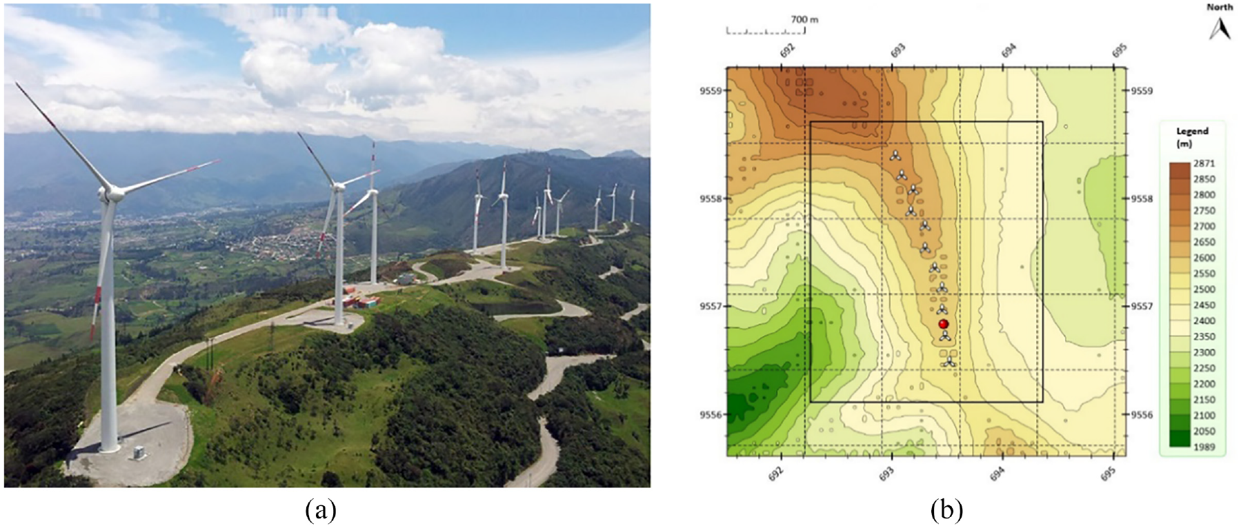
Villonaco wind farm: (a) panoramic view and (b) geographical coordinates (Ayala et al., 2017).

VWF consists of 11 wind turbines (WTs) GOLDWIND GW70 class “S,” with direct drive technology and permanent magnet synchronous generator of 1.5 MW nominal power (see Figure 1(b)). The location has an NNW-SSE orientation on the top of the Villonaco hill, in an approximate length of 2900 m. The farm was constructed at an approximate cost of USD 41.8 million, and has been operating since 2013 (Hernandez et al., 2016). This wind farm works under special conditions, with high annual average wind speed over 10 m/s, low air density of 0.89 kg/m³, and turbulence intensity of 0.15 (Reyes et al., 2017).

The regulatory framework of the electrical sector in force in Ecuador requires GENSUR EP, as the entity responsible for the operation of the VWF, to report daily and with a high degree of reliability, the estimate of electrical energy that VWF will produce the following day (Centro Nacional de Control de Energía, 2018).

Given that wind energy is a non-programmable form of generation, it is difficult to know with enough precision the total amount of wind energy that will be available the next day. Therefore, is a complex task to forecast the energy production of VWF, considering that wind is a random resource, with intermittence and large changes in short intervals of time.

In this context, the central objective of this study is to develop a wind power forecasting model, which will help to reduce the uncertainty in the estimation of energy production to be reported to the National Interconnected System of Ecuador, and will contribute to the improvement of the availability and reliability indicators the VWF.

The major contributions of this paper are summarized below:

A solution to the problem of forecasting the energy produced by VWF is proposed, through the use of Artificial Neural Networks (ANN), for which experimental tests are carried out based on the MLP, LSTM, CNN, and hybrid models.

A wind energy prediction approach is proposed for a wind farm like VWF, operating in extreme conditions, using as a model the data collected by the SCADA system of one of the wind turbines.

The remainder of this paper is structured as follows. Section “Related works” is dedicated to the analysis of works related to determining the state of the art. Section “Materials and methods” is dedicated to the materials and methods used in research. Section “Results and discussion” presents the results obtained and Section “Coclusion” presents the conclusions.

Related works

There is abundant scientific literature on wind energy forecasting models, the most important of which are based on meteorological models, advanced statistical models, models based on Computational Fluid Dynamics (CFD) and those using Artificial Intelligence (AI) tools (Marugán et al., 2018). In this section, we present a brief review of scientific articles on predictive models, using AI techniques published in the last 4 years. The related works are classified below according to the approach used.

Hybrid artificial intelligence approach

(Shahid et al., 2020) presents a novel method for accurate wind power prediction by applying computational intelligence approaches while exploiting Auxiliary Predictor (AxP) and Genetic Programming (GP)-based ensemble of Neural Networks (AxP-GPNN). The auxiliary predictor is built with the Radial Base Function (RBF) network and the Relevance Vector Machine (RVM) and several ANNs are used as base regressors. The ANNs are based on genetic programming (GP). Results are presented according to the statistical performance indices, MAE, standard deviation of error (SDE), and root mean squared error (RMSE). The authors normalize the power values between 0-1 to avoid any scale problems for the sake of comparison and to mask the physiognomies of different wind farms. In percentage terms, they present an improvement over other proposed models of up to 21.4% for RMSE, 20.6% for MAE, and 20.2% for SDE. In addition, in (Jafarian-Namin et al., 2019) the forecast of wind energy generation in an area is made through different methods, and then the most suitable one is recommended using some performance criteria. Box-Jenkins modeling and ANN modeling are used for forecasts in the last 12 months. The results showed that the improved ANN model, that is, using genetic algorithms (GA), obtains the best performance in predicting the power generation values. The algorithm works as follows: a few pairs of solutions are selected as parents to produce a group of children or (improved solutions). This reproduction is handled using two operators known as crossover and mutation. The reproduction process is applied to all selected pairs to create a new generation of improved solutions. This new population is then evaluated, and the breeding process is repeated until a convergence condition is satisfied. MAE, RMSE and others are used for comparison. It is important to mention that in numerous studies, the data collected by the SCADA system is used for the construction of WT prediction models. For example, in (Zheng et al., 2017), a new two-stage hybrid approach is proposed based on the combination of the Hilbert-Huang transformation (HHT), the GA and ANN for day-to-day wind energy prediction. The approach consists of two stages, the first using NWP information to predict the wind speed at the exact site of the wind farm, while the second stage maps the actual wind speed vis-a-vis the power characteristics delivered by SCADA. The proposed approach to predicting wind energy on a day-to-day basis is novel and effective. The average values of MAPE, MAE and forecast skill (FS) were 5.54%, 0.48%, and 42.67% respectively, exceeding the values of four other wind energy forecast models. Similarly, in (Li et al., 2019), a novel wind energy prediction method based on Extreme Learning Machine (ELM) with kernel mean p-power error loss is proposed, which can achieve lower prediction error, compared to Back Propagation Neural Network (BPNN). Further, according to authors, although the proposed method can achieve optimal predictive performance, there is still much work to be done in this field of research. Another approach use neural networks with random weights (NNRW) and linear combiner (Musikawan et al., 2020), in this approach the original time-series is decomposed into a collection of subseries by different decomposition techniques, each sub-series is modeled and predicted separately using (NNRW). Anthers authors uses the WRF model to obtain the numerical weather forecast and the gradient boosting decision tree (GBDT) algorithm to improve the near-surface wind speed post-processing results of the numerical weather model (Xu et al., 2020).

Multivariate models

In (Son et al., 2019), the authors used modified LSTM to predict wind energy in the short term. This method was compared with four multivariate methods derived from the combination of observation data. Among these models, the authors’ approach is more robust and accurate for predicting wind energy. Among the metrics used for the evaluation are RMSE and MAPE. The forecast of wind energy for an ultra-short period (>15 minutes to a couple of hours) is not an easy task, for which (Dong and Yang, 2018) presents an efficient solution to address the challenge based on historical data and Numerical Weather Prediction (NWP). The data are processed by reducing the dimensionality and the division of subsets and then using dynamically trained Adaptive Neutron-Fuzzy Inference System (ANFIS) with the algorithm of Particle Swarm Optimization (PSO). The proposed solution is evaluated through a case study of real wind farms and the numerical results clearly demonstrate its efficiency and predictive accuracy for an ultra-short period. In (Marulanda et al., 2020) this paper is focused on the generation of realistic wind power production scenarios in the long term and their results show that capturing the dependencies at the monthly level could improve the quality of scenarios at different time scales. Finally, in (Gilbert et al., 2020) they describe two methods for creating improved probabilistic wind power forecasts through the use of turbine-level data. The first is the engineering approach whereby deterministic power forecasts from the turbine level are used as explanatory variables in a wind farm level forecasting model, the second is a bottom-up hierarchical approach where the wind farm forecast is inferred from the joint predictive distribution of the power output from individual turbines.

There are many methods and approaches that have been published to date, most of them hybrid approaches that use artificial intelligence techniques; these methods are combined with different techniques or algorithms and have given promising results, therefore in present work a hybrid approach for wind power prediction is proposed.

Materials and methods

This section describes the characteristics of the data used, its organization and pre-processing, the methods for carrying out the regression and forecasting accuracy evaluation metrics.

Description of the SCADA data used

SCADA systems collects basic information with the use of sensors placed on key wind turbine components (e.g. bearing vibration, temperature, phase currents, wind speed, etc.) (Stetco et al., 2019). According to (Baltazar et al., 2019; Pliego Marugán and García Márquez, 2019; Stetco et al., 2019) the SCADA system normally records in a ten-minute resolution, some monitoring variables that can be grouped into three categories:

Wind parameters: direct wind measurements using an anemometer and a vane, such as wind speed, wind direction, etc.

Parameters related to energy conversion: such parameters are related to electricity output, for example, active power, generator rotation speed, pitch angle, etc.

Temperature parameters include external ambient temperature, gondola temperature, passer motor temperatures, etc.

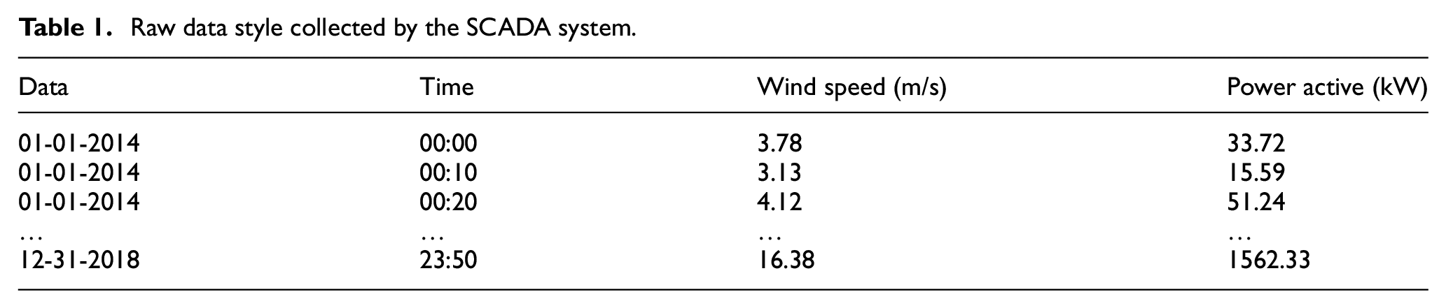
The data used in this study come from the SCADA system of WT 1 of VWF and covers a period of 5 years, from 01 January 2014 to 31 December 2018. Table 1 shows the parameter name and style of the raw data from the SCADA system used in this study.

Table 1.

Raw data style collected by the SCADA system.

Data	Time	Wind speed (m/s)	Power active (kW)
01-01-2014	00:00	3.78	33.72
01-01-2014	00:10	3.13	15.59
01-01-2014	00:20	4.12	51.24
…	…	…	…
12-31-2018	23:50	16.38	1562.33

Organization and preprocessing of data

According to (Marti-Puig et al., 2018), the SCADA data of the WT can contain errors caused by missing entries, uncalibrated sensors or human errors; it moreover mentions the finding from experimental results that using filters to eliminate outliers can decrease error in the train data set, but unfortunately, increases the error in the test data set.

The pre-processing of the data consisted of identifying the variables and the order in which they were found, in order to avoid inconsistencies in the consolidation of the data. The data set presented in Table 1 contains a total of 2,628,000 ten-minute measurements of both the Power Active and Wind Speed variables, of which an average of every 60 samples was taken to obtain 43,800 hourly measurements of the mentioned variables.

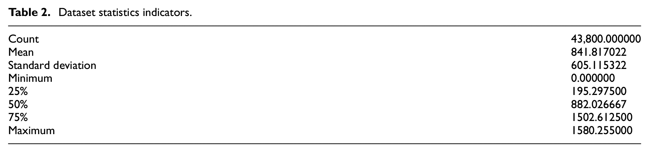
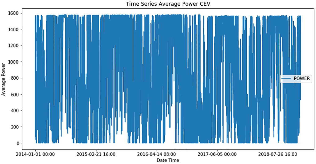
For the resulting dataset, the Power Active variable was extracted and used to create the neural network-based prediction models presented below. The statistical indicators of the dataset are shown in Table 2 and accordingly, its behavior can be visualized in Figure 2.

Table 2.

Dataset statistics indicators.

Count	43,800.000000
Mean	841.817022
Standard deviation	605.115322
Minimum	0.000000
25%	195.297500
50%	882.026667
75%	1502.612500
Maximum	1580.255000

Figure 2.

Hourly dataset.

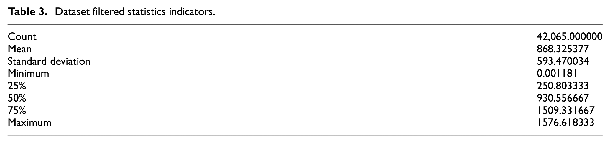
After the hourly dataset was obtained, the detection of outliers was performed through a Support Vector Machine (SVM) model to discard measurements that are not within the normal behavior of the data. As a result of this operation, Figure 3 highlights the red points to be eliminated, and Table 3 presents the main statistical indicators resulting from the filtered dataset.

Figure 3.

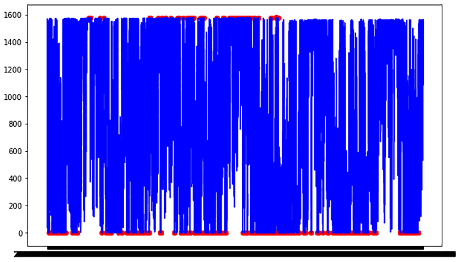
Outliers identified in the dataset through SVM.

Table 3.

Dataset filtered statistics indicators.

Count	42,065.000000
Mean	868.325377
Standard deviation	593.470034
Minimum	0.001181
25%	250.803333
50%	930.556667
75%	1509.331667
Maximum	1576.618333

As a result of the pre-processing, the final dataset contains 42065 Active Power measurements with the respective date and time of the measurement. Finally, we proceeded to divide the data, into the period from 2014 to 2017 for training and 75% of the year 2018 for the validation stage and 25% for testing, as shown in Figure 4.

Figure 4.

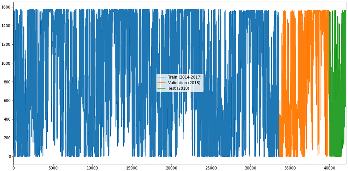
Filtered data set for training, validation, and testing.

With the data set divided into training and development sets, we proceed to convert the unsupervised data into supervised data, for this, we take a window that will determine the amount of characteristics or consecutive time samples that we will give as input to the models, while the label will be the subsequent time sample. For our new dataset has been chosen a window of 24 hours, as shown in Figure 5.

Figure 5.

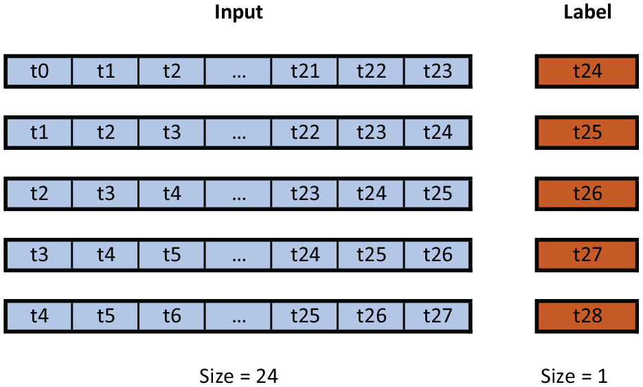
Processing of datasets to obtain supervised data.

In addition, once the data had been filtered, a standardization procedure was applied, which allowed the characteristics of the dataset to be transformed by scaling within a certain range. This operator scales and converts each characteristic of the training data set to a range between 0 and 1. The transformation is described by the following equation 1, according to (Ju et al., 2019).

X_{std} = \frac{X - Min (X)}{Max (X) - Min (x)}

(1)

X_{norm} = X_{std \cdot} (Max - Min) + Min

(2)

where:

$X_{std}$ = Standard deviation

$X_{norm}$ = Normalized input X

$Max, Min$ = Feature range (0,1)

Computational methods: Machine learning regression techniques

The problem of predicting the energy generated by a WF is addressed mainly from the point of view of time series, where different models and ANN architectures are applied to determine the energy generated in the short term and with the highest possible accuracy.

The time series are presented as one of the best models of the variation of energy in regular time intervals, with the objective of projecting the future values of the analyzed variable. For this, there are different methods, of which we can mention the physical, statistical and intelligent ones (Maldonado-Correa et al., 2020), being the methods based on AI, on which most of the research is focused. The NNAs are adapted to the non-linear behavior of the time series, and also take advantage of the presence of stationarity using hybrid models that characterize the energy production data.

Multi-layer perceptron

According to (Liu et al., 2018), multi-layer perceptron (MLP) is an ANN made of units arranged in layers with only forward connections to units in subsequent layers. In (Wasilewski and Baczynski, 2017), an approach to use MLP in short term wind forecasting is presented, based on three learning criteria, viz., Bias, MAE, RMSE, applied to the evaluation of each training and validation batch.

The MLP approach proposed in this study is shown in Figure 6. It can be seen that the input layer is fully connected and consists of 48 neurons that adapt to each of the hourly data for a corresponding day. These have a type activation rectified linear unit (ReLU) function, and two hidden, fully connected layers formed by 24 neurons with Sigmoid activation function, ending with an output layer fully connected formed by a neuron with default linear activation that adapts to the desired prediction.

Figure 6.

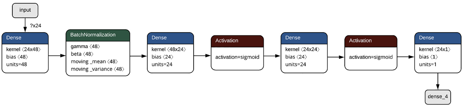
MLP for forecasting wind energy.

Long short-term memory

The long short-term memory (LSTM) networks are presented as an alternative and evolution of the NRNs that allow maintenance of the information-introducing loops in the network diagram, which generates a kind of memory of the previous states to affect the following states. Maintaining a relationship with the previous outputs allows them to be very adequate in the treatment of time series; however, this relationship is limited to short terms.

Moreover, the learning of long-term dependencies is one of the characteristics and advantages of the LSTM networks, since it can maintain its state in time through a memory cell. It is also able to regulate the amount of information from and to the cell, through non-linear gates (Hochreiter and Schmidhuber, 1997).

The model proposed in this study (see Figure 7), has an LSTM layer with a linear default activation function, with a kernel of 1×192 and a kernel of recurrence of 48×192, formed by 48 neurons and a dropout factor of 0.1%. It should be noted that dropout is a technique that avoids over-adjustment, by temporarily disconnecting certain neurons from the network and discarding their values. The next stage of Batch Normalization is used to increase the stability of the network. This normalization adjusts the output of a previous trigger layer by subtracting the batch mean and dividing it by the batch standard deviation. Next, we place two fully connected layers of 24 neurons and with hyperbolic tangential activation function to finally a fully connected layer of one neuron that presents the desired output.

Figure 7.

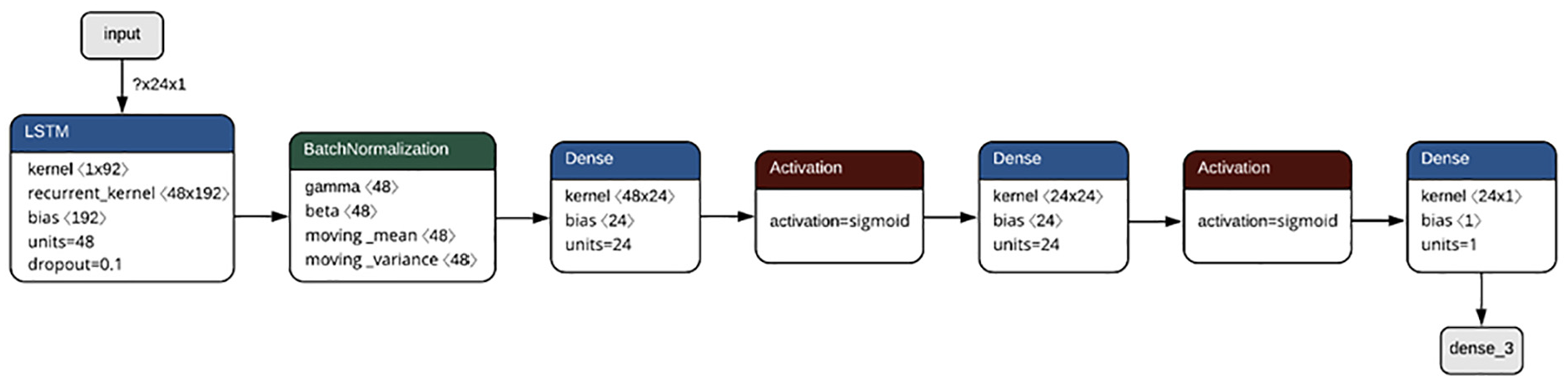
LSTM for forecasting wind energy.

Convolutional neural network

The convolutional neural networks (CNNs) are presented as an alternative for the prediction based on time series. In some cases, they are a better alternative to the LSTM networks, being able to improve their capacity of learning of nonlinear dependences by the application of deeper layers of filters (Borovykh et al., 2017).

The CNN approach proposed in this study (see Figure 8), uses a one-dimensional convolutional layer, a bank of 48 filters and a ReLU activation function, followed by a one-dimensional MaxPooling layer that allows reduction of the dimensionality, allowing assumptions about the characteristics obtained at the output of the filter sub-regions. Thereafter, we apply a dropout function to improve stability in the validation stage and through a flattening operation, we vector the output to pass it through a multilayer perception of four hidden layers and Sigmoid activation functions.

Figure 8.

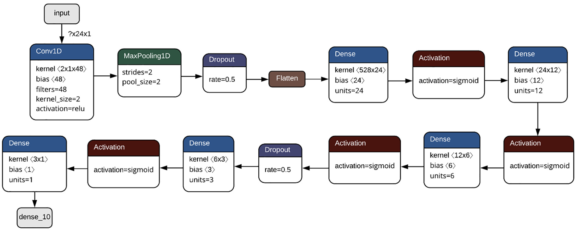
CNN for forecasting wind energy.

For the development of a functional prediction model for the VWF, the process of adjustment of the hyperparameters has been systematized, which allows to improve the precision and to reduce the percentages of error based on the evaluation metrics.

The MLP, LSTM, and CNN models have been evaluated and adjusted to present the best results with the VWF data, based on the selection of the hyperparameters through the following steps described in the flowchart in Figure 9.

Figure 9.

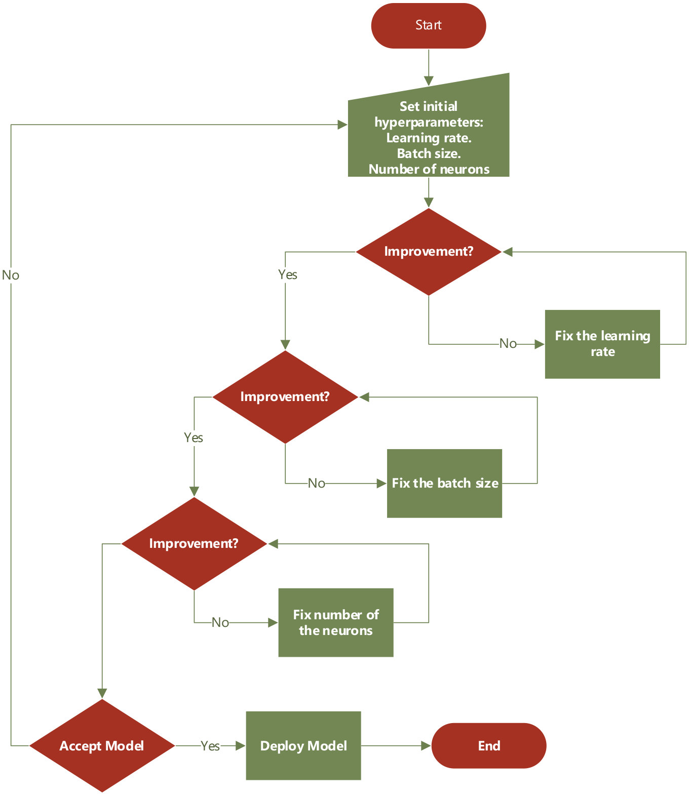
Flow diagram the hyperparameter adjustment of the models.

Forecasting accuracy evaluation metrics

In order to evaluate the prediction performance of our proposed model, we include some of them, such as: RMSE, MAE, SDE, MAPE, sum squared error SSE, normalized mean absolute error NMAE and FS (Shahid et al., 2020; Tian et al., 2018; Zheng et al., 2017).

The first one is the MSE, it can be expressed as:

MSE = \frac{1}{N} \sum_{i = 1}^{N} (y_{actual} - y_{predicted})^{2}

(3)

where $y_{actual}$ is actual value of wind power and $y_{predicted}$ is the forecast value obtained from our model. The next index that we use is the MAE, and is given as follows:

MAE = \frac{1}{N} \sum_{i = 1}^{N} | (y_{actual} - y_{predicted}) |

(4)

The next index is the MAPE, is given as follows:

MAPE = \frac{100}{N} \sum_{i = 1}^{N} | \frac{(y_{actual} - y_{predicted})}{\bar{y_{actual}}} |

(5)

where $\bar{y_{actual}}$ is mean actual wind power.

R and R2 are correlation coefficient and determination coefficient, respectively.

Results and discussion

Active power analysis

In Figure 10, we can compare the range and distribution of the average power (kW) for the first WT (WT1) from 2014 to 2018. We observe that there is a poorer variability in terms of power generation. The average power generation ranges from 750to 1212 kW. The best generation average was in 2015, at 1212.30 kW, its maximum interquartile range was in 2016 (IQR = 1374.887) and the minimum interquartile range was in 2015 (IQR = 1081.49). It is important to highlight that in 2017 there are outliers; therefore, this analysis allows to identify and clean these values to have a data set that serves best for prediction.

Figure 10.

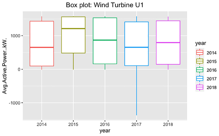
Boxplot of annually energy production by WT1.

Forecasting active power

The model architectures were built with the Api Keras and the Tensorflow library, using the Python programming language. When building the models, the same base input was defined for all of them, creating a window with the dataset measurements, with a length of 24 hours.

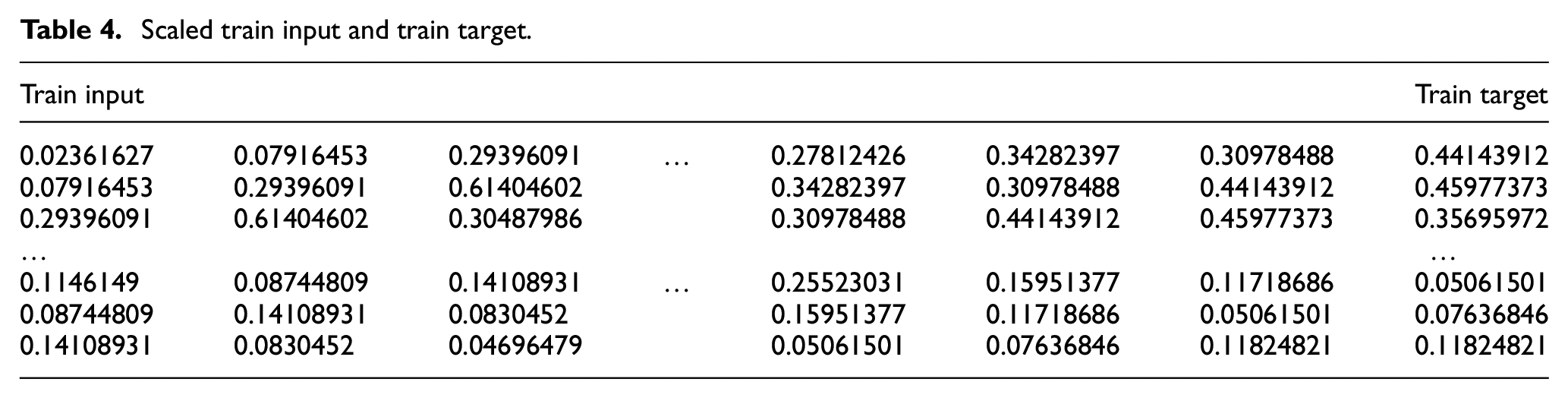
As can be seen in Table 4, each of the networks has a window of 24 consecutive hours as input. As regards the data corresponding to the 25th hour as output, it is sought that, given the previous 24 hours, the models are able to generate the next hour and in this way move the window throughout the entire training set.

Table 4.

Scaled train input and train target.

Train input							Train target
0.02361627	0.07916453	0.29396091	…	0.27812426	0.34282397	0.30978488	0.44143912
0.07916453	0.29396091	0.61404602		0.34282397	0.30978488	0.44143912	0.45977373
0.29396091	0.61404602	0.30487986		0.30978488	0.44143912	0.45977373	0.35695972
…							…
0.1146149	0.08744809	0.14108931	…	0.25523031	0.15951377	0.11718686	0.05061501
0.08744809	0.14108931	0.0830452		0.15951377	0.11718686	0.05061501	0.07636846
0.14108931	0.0830452	0.04696479		0.05061501	0.07636846	0.11824821	0.11824821

As explained above, the first model used in this study is an MLP. For their training, the hyper-parameters shown in Table 5 were adjusted.

Table 5.

MLP hyper-parameters.

Epochs	100
Hidden layer sizes	(512, 24)
Activation	(ReLu, sigmoid)
Solver	SGD
Loss	mean squared error
Learning rate	1E − 2

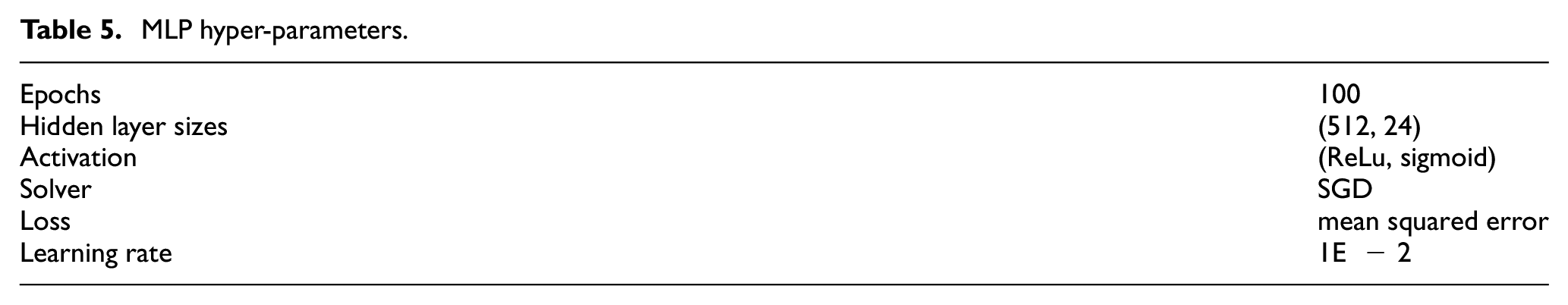
The hyperparameters presented are the result of applying the systematized process of adjustment, using which with the set of validation the parameters were obtained that optimized each model through tests with different combinations. First, initial values were fixed for the hyperparameters, the learning rate was adjusted leaving the other parameters fixed and observing the loss in the validation stage, then, the size of the batch was chosen to observe the loss of validation.

Continuing with the adjustment of the network, the number of epochs that have been optimized in the first part is kept fixed and we vary the amount of neurons in each hidden layer, in different tests, calculating the error in the validation stage and looking for the amount of optimal neurons that optimize the model.

The next parameter is that of the activation function of the neurons in the hidden layers, for which we have tested with functions, tangential, sigmoid and ReLu. After analyzing the validation error, the sigmoid function for each hidden layer is the one with the least error. In the result obtained for the validation batch, we observe that the prediction maintains the trend of the real value.

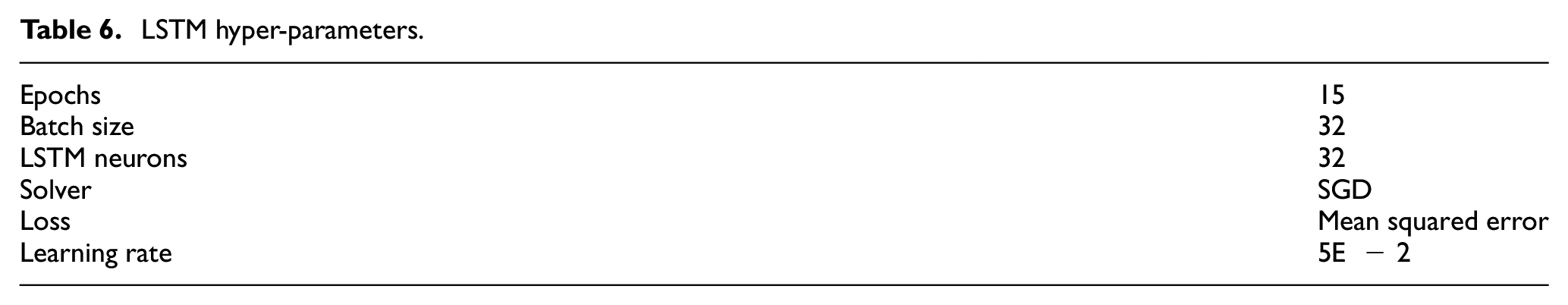
In Table 6, the hyper-parameters selected for the LSTM model can be seen. The selected parameters correspond to tests performed by varying the parameters of an LSTM network for different numbers of neurons and percentage dropouts. Additionally, an MLP was concatenated to improve the results, maintaining the trend of the real value for the validation batch.

Table 6.

LSTM hyper-parameters.

Epochs	15
Batch size	32
LSTM neurons	32
Solver	SGD
Loss	Mean squared error
Learning rate	5E − 2

Similarly, Table 7 shows the configuration of hyper-parameters for the CNN model. In the proposed CNN model, the structure differs from previous proposals in the presence of a one-dimensional convolutional layer, for which the parameters of activation function, number of filters, dropout and kernel dimension were varied until optimal results were achieved that minimized the model error. Additionally, a block of Flatten was considered to vectorize the results of the convolutional layer and take them as inputs for an MLP to determine the regression value. The result of the validation batch behaves according to the trend of the real values.

Table 7.

CNN hyper-parameters.

Epochs	10
Batch Size	32
Convolutional layers	2
Convolutional activation	ReLu
Number of filters	192, 72
Kernel size	5
Dropout rate	0.5
Fully connected layers	2
Solver	SGD
Loss	Mean squared error
Learning rate	5E − 2

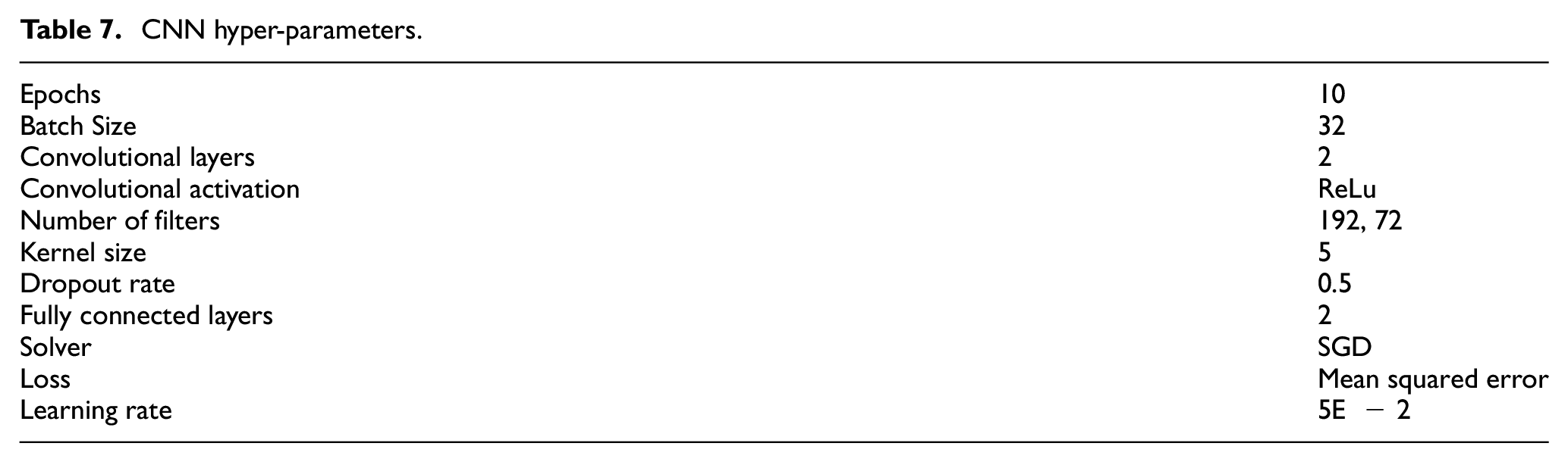
Figure 11 shows the result of 3 samples of a batch for the test set, where for different behaviors of the 24-hour input Windows, we can see the estimation of the following 24 hours made in this case by the CNN model.

Figure 11.

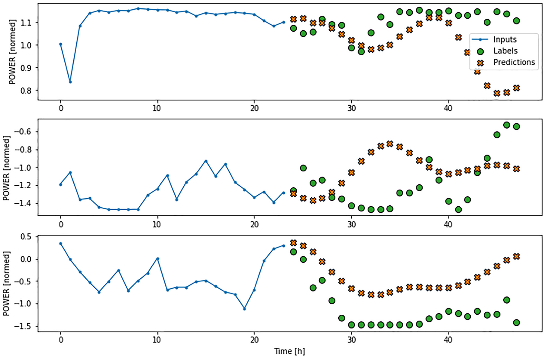
Samples of the 24-hour estimate using the CNN model.

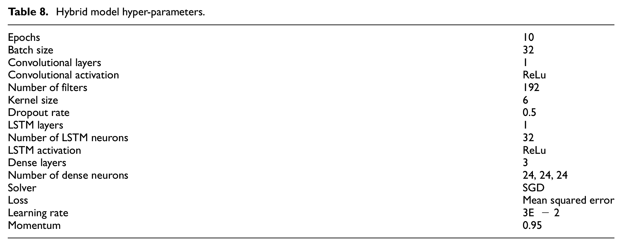
The adjustment of the different models, has allowed us to conclude in a hybrid model that allows to associate the different individual advantages, using two convolutional layers with 32 and 16 filters respectively, a kernel of size 5, two LSTM layers of 64 neurons each one and finally 2 Dense layers of 48 and 24 neuron respectively to present the prediction. For this model, the same procedure for adjusting the hyperparameters has been carried out again until it is optimized. Table 8 shows the optimized parameters for the hybrid model.

Table 8.

Hybrid model hyper-parameters.

Epochs	10
Batch size	32
Convolutional layers	1
Convolutional activation	ReLu
Number of filters	192
Kernel size	6
Dropout rate	0.5
LSTM layers	1
Number of LSTM neurons	32
LSTM activation	ReLu
Dense layers	3
Number of dense neurons	24, 24, 24
Solver	SGD
Loss	Mean squared error
Learning rate	3E − 2
Momentum	0.95

Comparative analysis

A comparison of the prediction results for the next 24 hours is shown in Figure 12. Here, it can be seen that the four proposed models have an acceptable behavior vis-a-vis what is expected, presenting greater problems in significant changes of slope, where it is appreciated that in accordance with the trend of the change, they make it through less pronounced changes.

Figure 12.

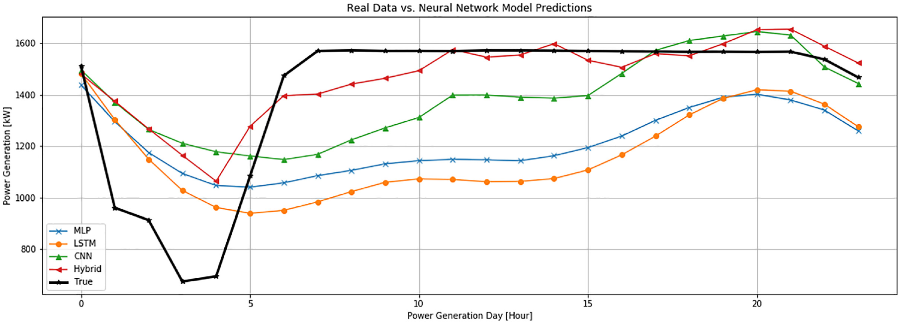
The prediction result of MLP, LSTM, CNN, and Hybrid.

We can also observe that the hybrid and convolutional models are the ones that best respond to extreme variations, with the hybrid being the one that does it best in a few hours. In addition, the Convolutional layer allows the hybrid model to mitigate changes in steep slopes.

Accuracy evaluation metrics

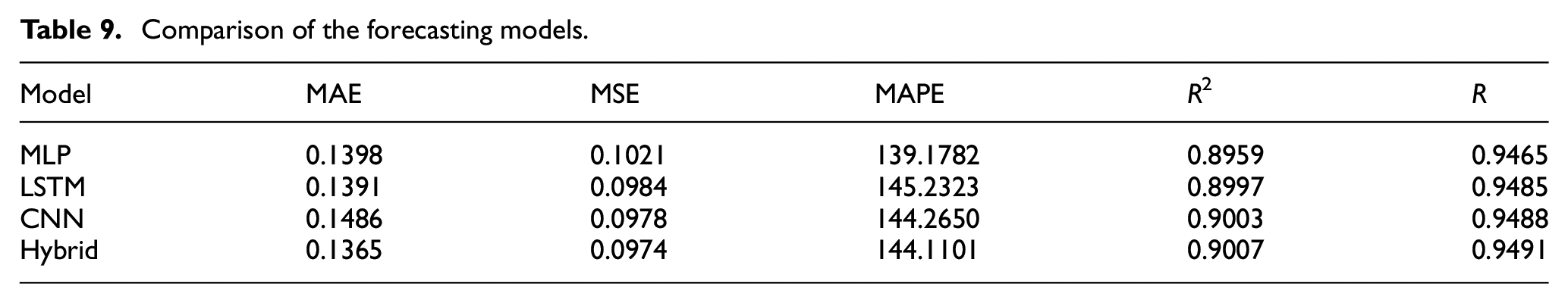
Table 9 shows the comparison of the performance indicators MAE, MSE, R, R2, and MAPE of the four prediction models applied in this article. It can be seen that the hybrid model has the lowest and therefore best values of MAE and MSE. Similarly, we can observe that according to R and R2, the prediction of the Hybrid and CNN models adjusts better to the real data, presenting a higher percentage of relation. Regarding MAPE, it measures the accuracy of predictions based on the percentage error of the model, which indicates that although the MLP model has obtained a lower value, the values of the hybrid and convolutional model are in an acceptable range.

Table 9.

Comparison of the forecasting models.

Model	MAE	MSE	MAPE	R ²	R
MLP	0.1398	0.1021	139.1782	0.8959	0.9465
LSTM	0.1391	0.0984	145.2323	0.8997	0.9485
CNN	0.1486	0.0978	144.2650	0.9003	0.9488
Hybrid	0.1365	0.0974	144.1101	0.9007	0.9491

These results can be compared to other results proposed in the literature for short-term active power forecasting that consider different methodologies and databases. For example, in (Srivastava and Tripathi, 2020), the importance of having an accurate wind energy forecast is mentioned. The authors use three AI methods, viz., Nonlinear Auto-Regressive Exogenous (NARX) network, Nonlinear Input-Output (NLIO), and Recurrent Neural Network (RNN) for short-term wind energy prediction, using data from the Kolkata region of India. The simulation results suggest that RNN can better predict wind energy than NARX and NLIO networks, according to MAE and RMSE assessment metrics.

Conclusion

The systematization of the adjustment of the parameters has allowed us to obtain results that improve on the models with base parameters, besides constituting a better vision for the selection of parameters of a hybrid model that takes advantage of the abstraction of characteristics of each model analyzed individually.

The comparison of the four proposed models allows us to see their functionality in the task of predicting the energy generated in the VWF. Each of the proposed architectures has its peculiarities with respect to the behavior of the wind farm, which allows us to intuit that the Hybrid model is presented as the most appropriate option by the values obtained of MAE, MSE, and R2, which were 0.1365, 0.0974, and 0.9007, respectively, outperforming three other wind power forecast models.

The data collected by the SCADA system of the WT is an important and abundant source of information for wind energy prediction models, which does not imply additional costs for the installation of sensors and hardware in the WT.

The authors found that there exist numerous studies on wind power forecasting in WTs using the SCADA data. However, no research appears to have been conducted on WFs located in mountainous terrains at high altitudes and operating under extreme conditions. In this sense, it is in the interest of the authors of this paper to develop a model for wind power forecasting to be applied in the VWF, which can be replicated in wind farms of similar characteristics.

Future work could consider the application of other architectures such as Generative Adversarial Network (GAN), for the prediction of energy generated in a wind power plant as well as the application of autoregressive models for the prediction. Additionally, we can test the behavior of our models with datasets from other wind power plants and analyze their behavior in the generalization of the predictions.

Footnotes

Acknowledgements

The authors acknowledge the support of Universidad Nacional de Loja by means of the research project “Artificial intelligence system for the short-term prediction of the energy production of the Villonaco wind farm. 26-DI-FEIRNNR-2019.” The authors would like to thank the Public Company “Corporación Eléctrica del Ecuador” CELEC EP GENSUR, for the information of its property provided. The SCADA data used to support the findings of this study have not been made available because of the nondisclosure agreement signed with CELEC EP GENSUR.

Declaration of conflicting interests

The author(s) declared no potential conflicts of interest with respect to the research, authorship, and/or publication of this article.

Funding

The author(s) received no financial support for the research, authorship, and/or publication of this article.

ORCID iDs

Jorge Maldonado-Correa

Marcelo Valdiviezo-Condolo

Marlon Santiago Viñan-Ludeña

References

Ayala

Maldonado

Paccha

, et al. (2017) Wind power resource assessment in complex terrain: Villonaco case-study using computational fluid dynamics analysis. Energy Procedia 107: 41–48.

Baltazar

Daniel

, et al. (2019) A review on neurocomputing based wind turbines fault diagnosis and prognosis. In: Proceedings - 2018 prognostics and system health management conference, PHM-Chongqing 2018 (eds Ding

Sánchez

, et al.), Chongqing, China, 26–28 October 2018, pp.437–443. Institute of Electrical and Electronics Engineers Inc.

Borovykh

Bohte

Oosterlee

(2017) Conditional time series forecasting with convolutional neural networks. arXiv preprint arXiv:1703.04691.

Centro Nacional de Control de Energía (2018) Operador Nacional de Electricidad. Available at: http://www.cenace.org.ec

Dong

Yang

(2018) Ultra-short term prediction model of wind power generation based on hybrid intelligent method. In: Chinese control conference, CCC, College of Electrical Engineering, Zhejiang University, Hangzhou, China, 25–27 July 2018, pp.9148–9153. IEEE.

Gilbert

Browell

McMillan

(2020) Leveraging turbine-level data for improved probabilistic wind power forecasting. IEEE Transactions on Sustainable Energy 11(3): 1152–1160.

Hernandez

Méndez

Maldonado-Correa

, et al. (2016) Modeling of a robust confidence band for the power curve of a wind turbine. Sensors 16(12): 2080.

Hochreiter

Schmidhuber

(1997) Long short-term memory. Neural computation 9(8): 1735–1780.

Jafarian-Namin

Goli

Qolipour

, et al. (2019) Forecasting the wind power generation using Box–Jenkins and hybrid artificial intelligence: A case study. International Journal of Energy Sector Management 13(4) 1038–1062.

10.

Sun

Chen

, et al. (2019) A model combining convolutional neural network and LightGBM algorithm for ultra-short-term wind power forecasting. IEEE Access 7: 28309–28318.

11.

(2019) Wind power prediction based on extreme learning machine with kernel mean p-power error loss. Energies 12(4): 673.

12.

Liu

Yang

Zio

, et al. (2018) Artificial intelligence for fault diagnosis of rotating machinery: A review. Mechanical Systems and Signal Processing 108: 33–47.

13.

Maldonado-Correa

Valdiviezo

Solano

, et al. (2020) Wind energy forecasting with artificial intelligence techniques: A review. In: International conference on applied technologies, 3 December 2019, pp.348–362. Cham: Springer.

14.

Marti-Puig

Blanco-M

Cárdenas

, et al. (2018) Effects of the pre-processing algorithms in fault diagnosis of wind turbines. Environmental Modelling & Software 110: 119–128.

15.

Marugán

Márquez

FPG

Perez

JMP

, et al. (2018) A survey of artificial neural network in wind energy systems. Applied Energy 228: 1822–1836.

16.

Marulanda

Bello

Cifuentes

, et al. (2020) Wind power long-term scenario generation considering spatial-temporal dependencies in coupled electricity markets. Energies 13(13): 3427.

17.

Musikawan

Sunat

Kongsorot

(2020) Wind power forecasting using a heterogeneous ensemble of decomposition-based nnrw techniques. ECTI Transactions on Computer and Information Technology 14(2): 122–138.

18.

Pliego Marugán

García Márquez

(2019) Advanced analytics for detection and diagnosis of false alarms and faults: A real case study. Wind Energy 22(11): 1622–1635.

19.

Reyes

Ibargüengoytia

Jijón

, et al. (2017) Wind power forecasting for the Villonaco wind farm using AI techniques. In: Pichardo-Lagunas

Miranda-Jiménez

(eds.) Advances in Soft Computing, MICAI 2016. Lecture Notes in Computer Science, vol. 10062. Cham: Springer, p. 228.

20.

Shahid

Khan

Zameer

, et al. (2020) Wind power prediction using a three stage genetic ensemble and auxiliary predictor. Applied Soft Computing Journal 90: 106151.

21.

Son

Yang

(2019) Hybrid forecasting model for short-term wind power prediction using modified long short-term memory. Energies 12(20): 3901.

22.

Srivastava

Tripathi

(2020) Predictive analysis of narx, nlio, and rnn networks for short-term wind power forecasting. In: Jain

Chaudhary

Taplamacioglu

, et al. (eds.) Advances in Data Sciences, Security and Applications. Lecture Notes in Electrical Engineering, vol. 612. Singapore: Springer, pp.45–62.

23.

Stetco

Dinmohammadi

Zhao

, et al. (2019) Machine learning methods for wind turbine condition monitoring: A review. Renewable Energy 133: 620–635.

24.

Tian

Wang

, et al. (2018) Artificial bee colony algorithm–optimized error minimized extreme learning machine and its application in short-term wind speed prediction. Wind Engineering 43(3): 263–276.

25.

Wasilewski

Baczynski

(2017) Short-term electric energy production forecasting at wind power plants in pareto-optimality context. Renewable and Sustainable Energy Reviews 69: 177–187.

26.

Ning

Luo

(2020) Wind speed forecast based on post-processing of numerical weather predictions using a gradient boosting decision tree algorithm. Atmosphere 11(7): 738.

27.

Zheng

Shi

Wang

, et al. (2017) Day-ahead wind power forecasting using a two-stage hybrid modeling approach based on SCADA and meteorological information, and evaluating the impact of input-data dependency on forecasting accuracy. Energies 10(12): 1988.