
Abstract
The accuracy of wind power prediction directly affects the operation cost of power grid and is the result of power grid supply and demand balance. Therefore, how to improve the prediction accuracy of wind power is very important. In order to improve the prediction accuracy of wind power, a prediction model based on wavelet denoising and improved slime mold algorithm optimized support vector machine is proposed. The wavelet denoising algorithm is used to denoise the wind power data, and then the support vector machine is used as the prediction model. Because the prediction results of support vector machine are greatly affected by model parameters, an improved slime mold optimization algorithm with random inertia weight mechanism is used to determine the best penalty factor and kernel function parameters in support vector machine model. The effectiveness of the proposed prediction model is verified by using two groups actually collected wind power data. Seven prediction models are selected as the comparison model. Through the comparison between the predicted value and the actual value, the prediction error and its histogram distribution, the performance indicators, the Pearson’s correlation coefficient, the DM test, box-plot distribution, the results show that the proposed prediction model has high prediction accuracy.
Introduction
Wind energy has become an important renewable energy that can be developed and utilized on a large scale, and has attracted more and more attention (Barra et al., 2021). In recent years, with the popularization of wind power equipment manufacturing technology and the continuous expansion of wind turbine manufacturers, the price of wind turbine has gradually decreased. Many countries take wind power generation as the main energy for future development to formulate power development plans. With the large-scale production of wind turbine manufacturing, wind power has become the fastest developing clean and renewable energy in the world. However, there are some problems in wind power grid connection. The main reason is the random fluctuation and uncontrollability of wind power (Ai et al., 2020). It is difficult to predict the scale and change trend of wind power output in the future, which makes the power system operators unable to deal with the violent wind power fluctuations and make the decision-making response of dispatching control and power transaction quickly and accurately. Therefore, accurate prediction of wind power can effectively alleviate the strong uncertainty brought by large-scale wind power grid connection to power system operation, which has important economic significance and academic value (Akhtar et al., 2021; Tian et al., 2018).
According to whether the prediction results are determined or uncertain, wind power prediction can be divided into deterministic prediction and probabilistic prediction. The deterministic prediction of wind power means that only a specific value is given as the prediction result for each sampling time in the future. In a statistical sense, the determined value is the expected value of the possible wind power prediction results at that sampling time. The result form of deterministic prediction is simple, intuitive, and easy to understand, and the error evaluation is relatively direct. It only needs to compare with the measured value in the same period to obtain the error value, but its disadvantage is that it provides insufficient prediction information and cannot provide sufficient decision-making information support for power system dispatching operation and market transaction. In fact, due to the uncertainty of wind power generation, the prediction results of wind power generation should also contain additional uncertainty information. The probabilistic prediction of wind power provides the range of possible fluctuation of predicted value at a certain confidence level, that is, the range of prediction error. Probability prediction shall ensure that the fluctuation range of prediction results is as small as possible. But at the same time, the range can cover the actual value. Deterministic prediction can directly evaluate the prediction performance through the error between the actual value and the predicted value of wind power. The probabilistic prediction obtains the object probability distribution of the predicted wind power, but the actual probability distribution of the wind power object is difficult to obtain in reality. Therefore, it is necessary to put forward targeted evaluation indexes for the probability prediction results. As a method to quantify the prediction uncertainty, the prediction distribution described by the probabilistic prediction results should be as close as possible to the real distribution of the wind power object. The common indexes of probabilistic prediction include reliability index, sharpness index, and continuous ranked probability score index, and so forth. In this study, the deterministic prediction of wind power is discussed.
According to the characteristics of the prediction model, the deterministic prediction of wind power can be divided into persistence model, physical model, statistical learning model, intelligent model, and combination model (Tian, 2021).
The persistence model, also known as naive predictor, is a prediction model that uses the known wind speed or wind power value as the prediction value at future time to be predicted (Weber et al., 2019). Due to the existence of physical inertia, the model can achieve very good results in the ultra-short-term wind power prediction with the prediction horizon within 1–2 hours. Therefore, it is used as a reference model to compare with various prediction models. The improvement range of various prediction models compared with the persistence model can be used as an evaluation index. This persistence model is also used in the short-term wind power prediction and evaluation system.
The physical model analyzes and models the actual atmospheric physical characteristics. Generally, the atmospheric wind speed information given by the meteorological center will be transformed into the meteorological conditions around the wind farm to be predicted. As a typical physical prediction model, numerical weather prediction (NWP) obtains conclusions by solving complex mathematical models including meteorological data such as temperature, pressure, topography, and geomorphology (Hu et al., 2021b). Due to the large amount of calculation, NWP is generally realized by simulating atmospheric motion by supercomputer, and the algorithm complexity and cost are high. On the other hand, due to the low daily update frequency of meteorological data, NWP is more suitable for medium-term and long-term wind power prediction with a time scale >6 hours (Bossavy et al., 2013).
The basic idea of the prediction model based on statistical algorithm is to establish a mapping relationship between the system input (NWP, historical measured operation data) and wind power. Usually, this mapping is a linear relationship that can be explicitly represented by a function. Auto regressive (AR) model is a widely used statistical model in the initial stage of the development of wind power prediction (Feng et al., 2015). AR is regarded as a typical statistical model for wind speed prediction and wind power prediction. In addition, auto regressive moving average (ARMA) model is also widely used in wind power prediction. It defines the predicted value of wind power as a linear function of actual value (Li et al., 2014). ARMA has strict requirements for the stationary of time series, but the wind power time series often cannot meet the stationary conditions. In order to solve the non-stationary of wind power time series, auto regressive integrated moving average (ARIMA) model can be used for prediction (Chen et al., 2010). The prediction accuracy of the statistical model decreases with the increase of prediction time scale, and is sensitive to parameters. The prediction accuracy of the stationary time series is higher, and the prediction accuracy of unstable wind is lower. Because the calculation process and structure of the statistical model are relatively simple and stable in the short-term scale, it is also used as a benchmark model in the research to evaluate the prediction effect of other models.
In addition to the prediction models mentioned above, intelligent learning model, such as artificial neural network (Abedinia et al., 2020; Dorado-Moreno et al., 2017; Wan et al., 2013; Wang et al., 2020), support vector machine (Li et al., 2019), least squares support vector machine (Ding et al., 2021; Gan and Ke, 2014), etc., are developing most rapidly in the field of wind power prediction. The intelligent learning model establishes the relationship between input variables and output variables through the learning and training of a large number of historical operation measured data. It is a black box model rather than an explicit description in the form of analytical method. In recent years, some models based on deep learning mechanism have also been applied to the prediction of wind power. This includes recurrent neural network (Liu et al., 2021), long short-term memory (Han et al., 2019), gate recurrent unit (Ding et al., 2019), etc. The model built by intelligent learning is usually a nonlinear model. It can more accurately fit the nonlinear relationship and non-stationary between wind power and wind speed time series itself, reflect the fluctuation characteristics of wind power, and has high prediction accuracy. Because the training of intelligent learning model is based on a large number of historical data, compared with the traditional statistical model, the model is more complex and the training speed is slow.
Because various prediction models have some inherent limitations in their basic theories, and the prediction effects are different in different prediction situations. In order to optimize the prediction process and improve the prediction accuracy, the combination prediction of comprehensive multiple models has gradually become a more popular research idea. The combination prediction model can comprehensively use the statistical information of each single prediction model, establish the combination prediction model according to the technical characteristics and advantages of each model through the idea of complementary advantages, overcome the limitations of the single prediction model, and effectively reduce the probability of large errors. Typical combination prediction models include combination prediction model based on weight coefficient (An et al., 2021; Sun et al., 2019), combination prediction model combined with data preprocessing (Wang et al., 2019; Zhang et al., 2019a), combination prediction model based on model parameter optimization (Qin et al., 2021), etc. A large number of studies show that the prediction accuracy of the combination prediction model has been improved compared with the single prediction model.
Among the machine learning methods, SVM is an advanced learning method, which is especially suitable for modeling in the case of small samples. The nonlinear mapping ability of SVM can effectively predict the wind power data with complex characteristics. There is a lot of noise in the actual wind power data, which will reduce the final prediction accuracy. In this paper, a wavelet denoising (WD) algorithm is adopted to process the wind power, and the SVM model is established and predicted by using the wind power data generated after WD processing. The successful introduction of WD algorithm can effectively avoid the adverse interference of noise on wind power in the modeling process, and effectively improve the prediction accuracy of the model. At present, in the process of wind power prediction using SVM, there are some difficulties in the selection of parameters. The appropriate parameter value is the fundamental to the accuracy of prediction results. Therefore, the optimization of SVM model parameters is one of the key contents of the research. In recent years, many scholars have introduced genetic optimization algorithm (Zhang et al., 2019b), particle swarm optimization algorithm (Lu and Liu, 2015), gray wolf optimization algorithm (Lu et al., 2020), and other algorithms into SVM model optimization to improve the prediction accuracy of the model. However, most of these optimization algorithms have the shortcomings of local optimization and difficult to obtain the best parameters, so the prediction accuracy needs to be further improved. As a Meta heuristic algorithm, slime mold algorithm (SMA) has good optimization performance. In this paper, an improved SMA algorithm (ISMA) is designed by introducing random inertia weight mechanism, which further improves the convergence speed of the algorithm, and ISMA is applied to the optimization of SVM parameters. The effectiveness of the designed prediction model is verified by using the actually collected wind power data. In conclusion, the main innovations of this paper are as follows.
WD algorithm is used to denoise the wind power data to reduce the impact of interference on the modeling process and improve the final prediction accuracy.
The random inertia weight mechanism is introduced into SMA algorithm to realize ISMA, which improves the convergence speed and optimization effect.
ISMA is used to optimize the parameters of SVM. The optimized SVM is used to predict the wind power after WD processing.
The rest content of the paper is arranged as follows. Section 2 introduces the knowledge of WD algorithm and the WD processing of wind power; Section 3 introduces the process of ISMA optimized SVM model. Section 4 gives the implementation process of the designed prediction model. The case studies are given in Section 5. The conclusions and future work are summarized in Section 6.
WD processing of wind power
Wind power data is collected periodically and can be regarded as a time series. Due to the interference of various external factors, non-stationary data signals will be formed, and a variety of noise will exist in wind power time series. The wind power with noise is shown in equation (1).

where
After analyzing the wind power with noise signal, selecting the appropriate wavelet function and the number of decomposition layers are the key steps in the noise reduction process. In general, Mallat decomposition is widely used, including wavelet decomposition and signal reconstruction. The decomposition process is shown in equation (2).

where
In the process of wavelet denoising of wind power, the selection of threshold function has an important impact on signal denoising. Among many wavelet basis functions, Daubechies (DB) wavelet has compact support, high normality, and orthogonally in time domain, and has mature Mallat fast algorithm. That is commonly referred to as DB(N) wavelet. With the increase of length N, the frequency division ability of wavelet increases obviously, and the amount of calculation increases at the same time. Therefore, in practice, we should reasonably select the appropriate N to ensure the balance between decomposition performance and real-time performance. In DB wavelet series, DB4 wavelet has the shortest time window and the highest time resolution compared with other wavelets. It can be applied to the denoising of non-stationary signals. In this paper, DB4 orthogonal wavelet is used to decompose the wind power time series by four layers of wavelet, and the soft threshold function is selected to quantify the wavelet coefficients. In this way, on the premise of ensuring the accuracy, the noise information can be effectively suppressed, and then the ideal denoising effect can be realized. The soft threshold function is as follows:

where
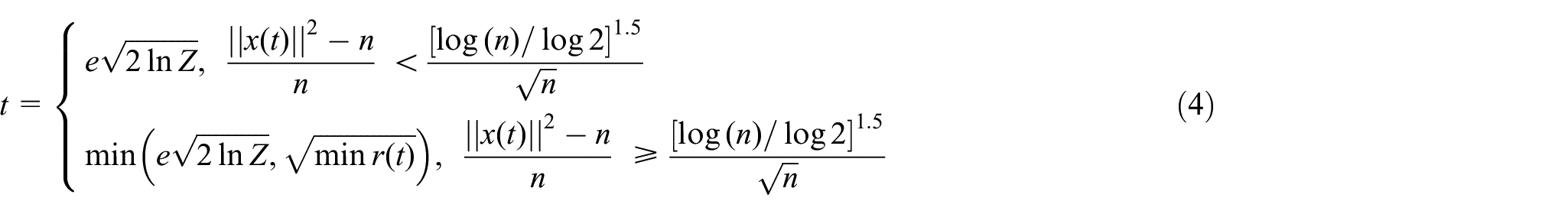
where e is the standard deviation of the additional noise signal, and Z is the length of the signal. Through wavelet denoising, the adverse interference such as peak and sudden change of wind power noise is eliminated, the trend of the original waveform is retained, the trend of wind power is more regular, the correlation information of wind power data is enhanced, and the problem that the subsequent modeling and prediction cannot be accurately carried out due to the existence of noise is solved.
ISMA optimized SVM
In this section, we introduce SVM model, ISMA algorithm and how to use ISMA to optimize SVM to obtain the best model parameters.
SVM
SVM can solve the nonlinear problem well. It can map the training samples from the original space to a higher dimensional space, so that the samples are linearly separable in this space (Gu et al., 2021). Therefore, the nonlinear SVM prediction function model can be expressed as shown in equation (5).

where w represents the vector of the weight system, b represents the bias vector, and

By minimizing, the parameters w and b can be obtained. In equation (6), C is the penalty factor,
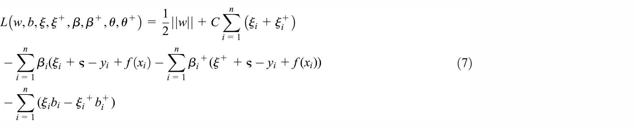
where

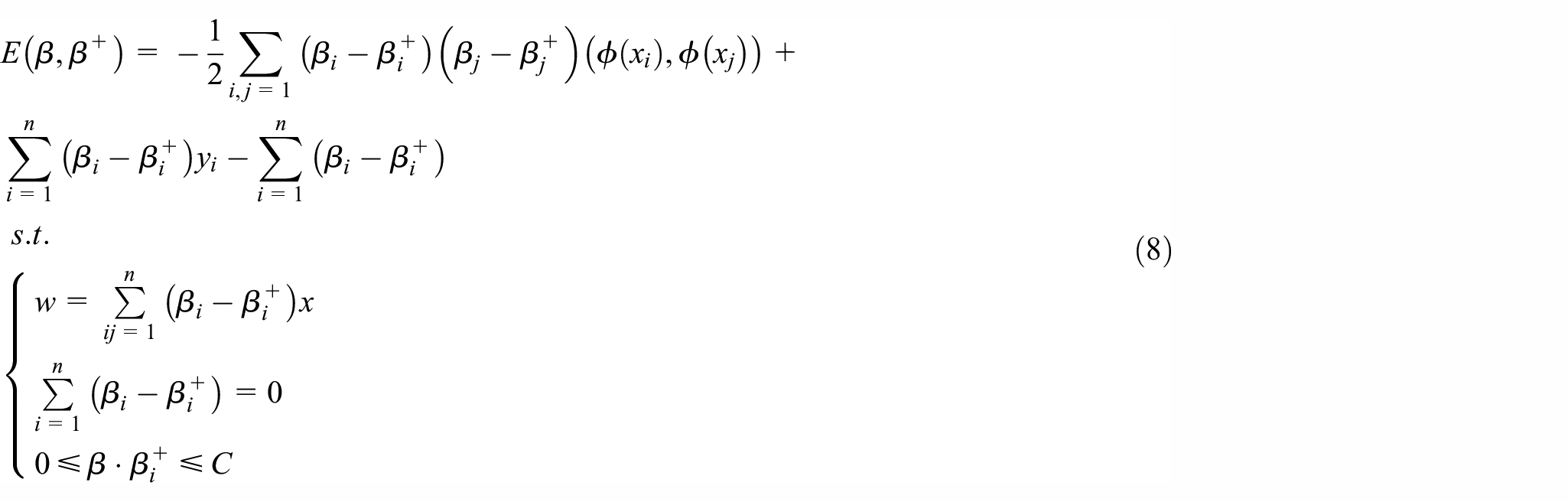
In order to avoid dimension disaster and save computation, kernel function

In order to map the sample data to a higher dimensional space, the radial basis function is selected as the kernel function of SVM. Radial basis function not only has the characteristics of mapping samples to high-dimensional space, but also has the advantages of few parameters. It is defined as follows:

where
ISMA
The performance of SVM model is greatly related to the penalty factor C and the selection of parameter

where LC and UC are the upper and lower bounds of the search range respectively. The parameter value range of mb is

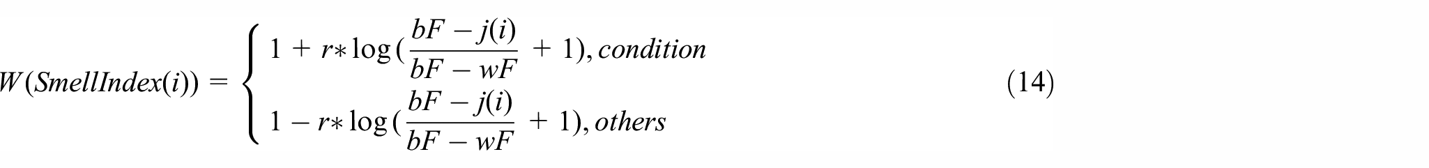

where condition represents the first half of the population in the ranking of
In this paper, the random inertia weight mechanism is used to improve the convergence speed of standard SMA. The introduction of random inertia weight is to obtain the inertia weight by introducing random distribution. The equation (16) of random inertia weight is applied to the position update formula of SMA to avoid the disadvantage of insufficient local searching capacity in the early and later stages of iteration. The improved population location updating mechanism is shown in the following equation (17).


where
SVM optimization based on ISMA
The process of SVM parameter optimization using ISMA is as follows. The penalty factor C and radial basis kernel function parameter

where N is the number of samples,

Proposed prediction model
Based on the introduction of the above basic knowledge, the flow chart of the wind power prediction model based on WD and ISMA optimized SVM proposed in this paper is shown in Figure 1.

The flow chart of the proposed wind power prediction model.
As can be seen from Figure 1, the specific implementation process of the designed prediction model is as follows.

Case study
The validity of the prediction model is verified by the actual wind power data. Compared with other benchmark prediction models, the comparison results fully show the effectiveness of the proposed prediction model.
Data set
In this study, two wind power data sets are collected from Manjing wind farm in Shangyi County, Zhangjiakou City, Hebei Province, China, from 2013 to 2015. In Manjing wind farm, there are totally 122 sets of wind turbines with a single unit capacity of 2.5 MW and a total capacity of 305 MW. The first wind power data set is from No. 7 wind turbine. The sampling time is 10 minutes and is named data set A. The second wind power data set is from No. 10 wind turbine. The sampling time is 30 minutes and is named data set B. The sample size of both data sets is 1000. The data set is divided into two parts, the first 80% of 800 groups of data as the training set, and the last 20% of 200 groups of data as the test set. WD algorithm is introduced to reduce the noise of wind power data set. The original data of data set A and the results after DB4 WD noise reduction are shown in Figure 2. The original data of data set B and the results after DB4 WD noise reduction are shown in Figure 3.
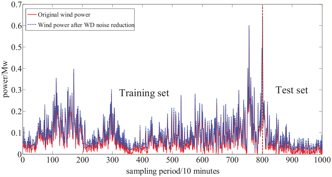
The original data of data set A and the results after DB4 WD noise reduction.

The original data of data set B and the results after DB4 WD noise reduction.
It can be seen from Figures 2 and 3 that the wind power time series has strong nonlinear, non-stationary and fluctuating characteristics, and there will be great differences in the wind power values at the two sampling times, which brings great difficulties to its modeling and prediction. On the other hand, it can be seen from the comparison before and after noise reduction in Figures 2 and 3 that since the wind power data before noise reduction is time-varying, there are parts polluted by noise. Compared with the data without noise reduction, the wind power data after noise reduction has the characteristics of stronger correlation, less volatility, and more regular trend. Through the simulation comparison below, it can be seen that the introduction of wavelet denoising is an effective method, which lays a foundation for complex and changeable wind power prediction.
Performance indicators
In order to verify the prediction accuracy of the wind power prediction model, the following eight performance indicators are introduced to measure the prediction effect of the prediction model (Tian and Chen, 2021).
RMSE

Mean absolute error (MAE)

Mean absolute percentile error (MAPE)

Relative root mean square error (RRMSE)

Square sum error (SSE)

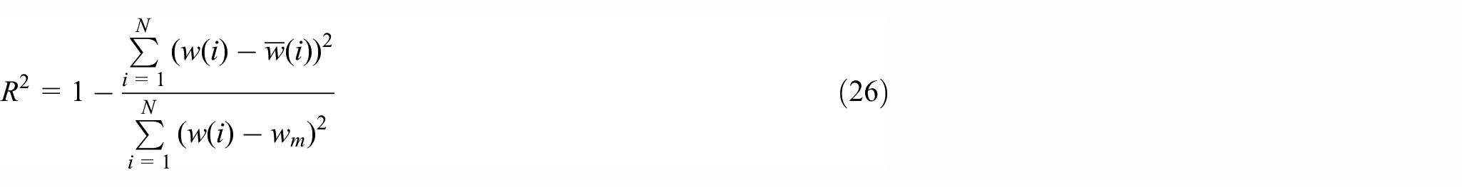
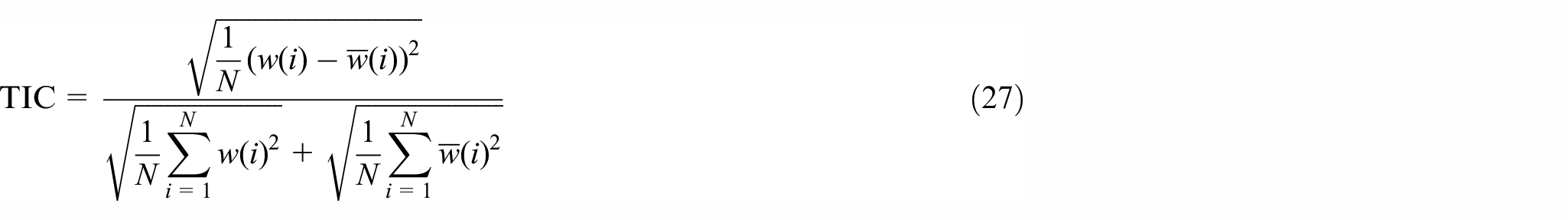
Theil inequality coefficient (TIC)
The index of agreement (IA)

where, N is number of samples,
At the same time, the Pearson’s test is introduced to test the accuracy of prediction from the statistical point of view (Mao, 2020). Pearson’s test can reflect the correlation strength between the actual value and the predicted value. If the Pearson correlation coefficient is closer to 1, the stronger the correlation between the actual value and the predicted value is, the better the prediction effect is. Otherwise, the closer the Pearson correlation coefficient is to 0, the worse the prediction effect of the prediction model is.
Finally, in order to prove the prediction performance, the Diebold-Mariano (DM) test is used to test prediction accuracy from the hypothesis test. The definition of DM test is as the follows. The hypothesis tests are:


The DM test statistic value equals the next.
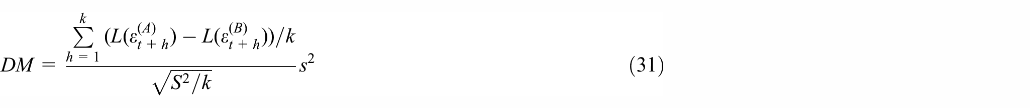
where

where

Comparison models
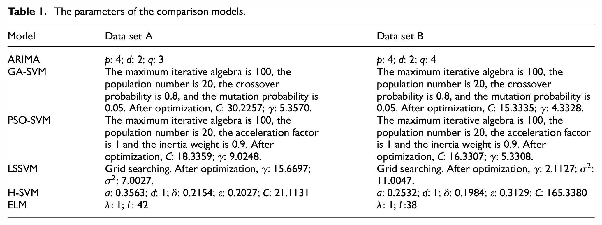
In order to test the prediction performance of the proposed prediction model, this paper selects seven prediction models including the persistence model (Weber et al., 2019), ARIMA (Chen et al., 2010), genetic algorithm optimized SVM (GA-SVM) (Zhang et al., 2019b), particle swarm algorithm optimized SVM (PSO-SVM) (Lu and Liu, 2015), LSSVM (Gan and Ke, 2014), hybrid kernel function SVM (H-SVM) (Tian et al., 2018), and extreme learning machine (ELM) (Wan et al., 2013) as the comparison model. The specific parameters of these comparison models are shown in Table 1 below (the persistence model does not need parameter setting. In this paper, the current value is regarded as the predicted value of the next sampling time in the future).
The parameters of the comparison models.
Results
For the prediction model in this paper, the initial population number of ISMA is set to 20, the dimension is 2, the value of parameter Z is set to 2, the maximum number of iterations is set to 100, the upper bound of C is 100 and the lower bound is 0.1, the upper bound of
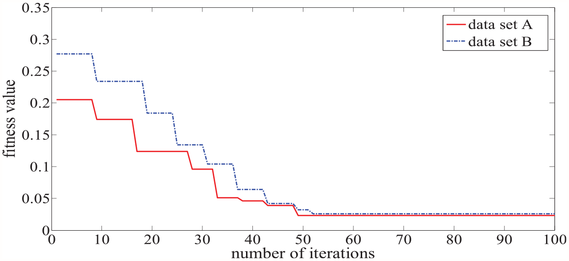
The ISMA optimization fitness curve of data set A and data set B.
After obtaining the best parameters of SVM through ISMA, 200 groups of test set data are predicted. At the same time, the comparison models using parameters given in Table 1 are used to predict the same test set. For data set A, the comparison curve between the predicted value of the proposed model and the comparison models and the actual value of wind power is shown in Figure 5. For data set B, the comparison curve between the predicted value of the proposed model and the comparison models and the actual value of wind power is shown in Figure 6. From the comparison results in Figures 5 and 6, compared with other comparison models, the predicted value of the model in this paper can better fit the change trend of wind power data and better reveal the internal evolution law of wind power time series. The comparison results show that the proposed prediction model has better fitting ability.
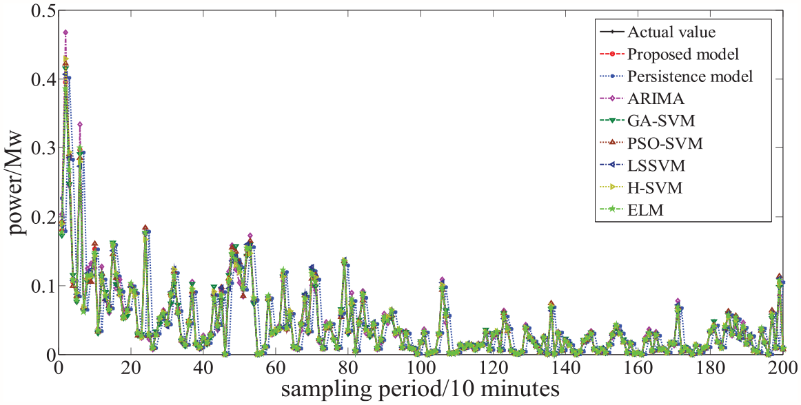
The actual value and prediction value comparison between the proposed model and comparison models for data set A.
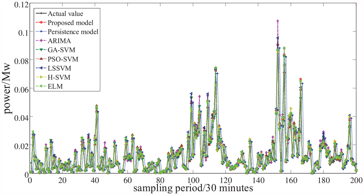
The actual value and prediction value comparison between the proposed model and comparison models for data set B.
Figures 7 and 8 show the distribution of prediction errors of these prediction models for data set A and data set B, respectively. From the results of these two figures, it can also be seen that the prediction error of the proposed model in this paper is smaller than that of the comparison model, which further illustrates the effectiveness of the proposed prediction model.
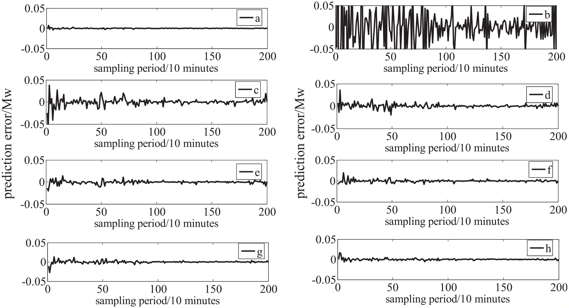
The prediction error comparison between the proposed model and comparison models for data set A: (a) proposed model, (b) persistence model, (c) ARIMA, (d) GA-SVM, (e) PSO-SVM, (f) LSSVM, (g) H-SVM, and (h) ELM.

The prediction error comparison between the proposed model and comparison models for data set B: (a) proposed model, (b) persistence model, (c) ARIMA, (d) GA-SVM, (e) PSO-SVM, (f) LSSVM, (g) H-SVM, and (h) ELM.
Figures 9 and 10 show the histogram of the prediction error distribution of these models for dataset A and dataset B, respectively. It can be seen from Figures 9 and 10 that the prediction error histogram distribution of the proposed prediction model is more concentrated around the abscissa zero, which means that the number of smaller prediction errors is more than that of larger prediction errors. Therefore, the prediction error histogram distribution of the proposed prediction model is centralized rather than decentralized, and the prediction performance is better than other models.

The histogram of the prediction error distribution for data set B: (a) proposed model, (b) persistence model, (c) ARIMA, (d) GA-SVM, (e) PSO-SVM, (f) LSSVM, (g) H-SVM, and (h) ELM.

The histogram of the prediction error distribution for data set B: (a) proposed model, (b) persistence model, (c) ARIMA, (d) GA-SVM, (e) PSO-SVM, (f) LSSVM, (g) H-SVM, and (h) ELM.
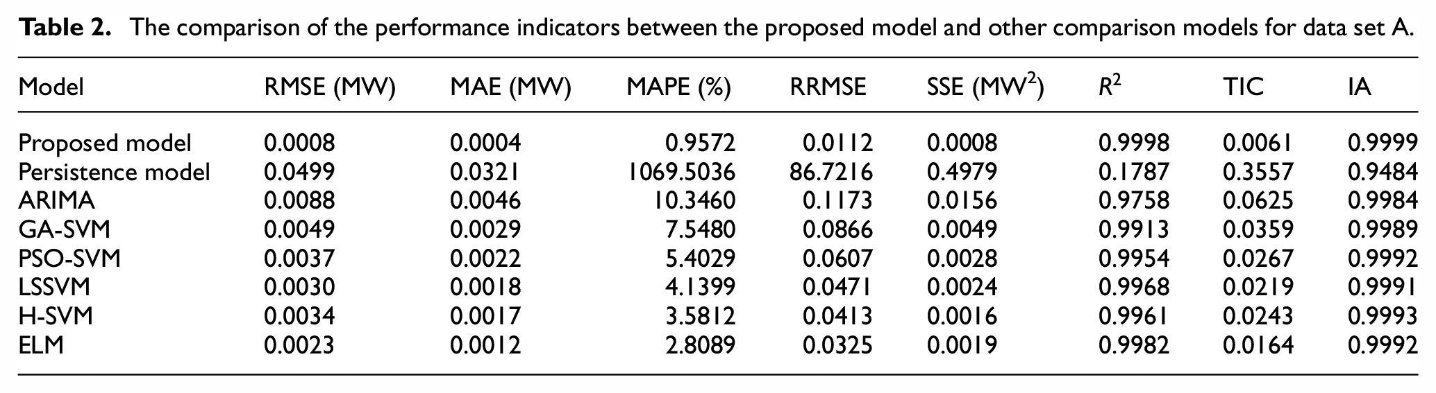
The following Tables 2 and 3 shows the comparison of the eight performance indicators between the proposed model and other comparison models for data set A and data set B, respectively. It can be seen from the results in two tables that the performance indicators of the proposed model are better than other comparison models. Specifically, as can be seen from the comparison results in these two tables, RMSE, MAE, MAPE, RRMSE, SSE, and TIC values of the proposed prediction model are smaller than the other comparison models. The smaller the values of these performance indicators, the better the prediction performance of the prediction model. Meanwhile,
The comparison of the performance indicators between the proposed model and other comparison models for data set A.
The comparison of the performance indicators between the proposed model and other comparison models for data set B.
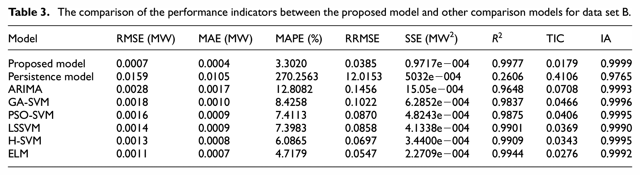
Table 4 gives the results of the Pearson’s test between the proposed model and other comparison models. The closer the Pearson’s correlation coefficient is to 1, it indicates that the actual value of the prediction model has a stronger linear relationship with the predicted value, which indicates that the prediction model has better prediction ability for the data object to be predicted. On the contrary, if the Pearson’s correlation coefficient is closer to 0, the linear relationship between the predicted value of the prediction model and the real value of the data object is weaker, that is, the prediction ability of the prediction model is poor. The results in Table 4 clearly show that the result of Pearson’s test of the proposed prediction model is higher than those of the other prediction models.
The Pearson’s test results between the proposed model and comparison model.

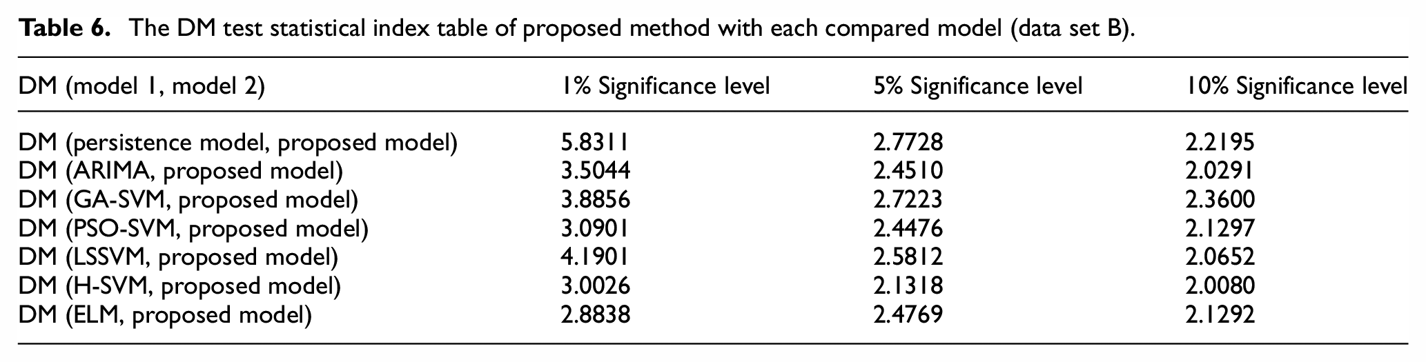
The DM test values calculated by the square error loss function with 1%, 5%, and 10% significance level are listed in Tables 5 and 6 for data set A and data set B. For two prediction models, if DM (model 1, model 2) is >0, the performance of the model 2 is better than model 1. On the contrary, if its value is <0, it indicates that the performance of model 1 is better than that of model 2. From the results in Tables 5 and 6, the DM test values between other models and the proposed model are >0, the proposed prediction model significantly outperforms the other prediction models at the same significance level. Thus, it can reasonably be concluded that the proposed prediction method is superior to the other models.
The DM test statistical index table of proposed method with each compared model (data set A).

The DM test statistical index table of proposed method with each compared model (data set B).
Finally, in order to more intuitively reflect the size of the prediction error, this paper also adopts the box-plot to graphically present the prediction error, as shown in Figures 11 and 12. Through the box-plot, it can intuitively see that the model proposed in this paper has smaller errors and higher prediction accuracy, and the model proposed in this paper is excellent.
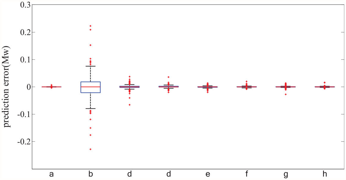
Box-plot of prediction errors comparison for data set A (a: proposed model; b: persistence model; c: ARIMA; d: GA-SVM; e: PSO-SVM; f: LSSVM; g: H-SVM; h: ELM).
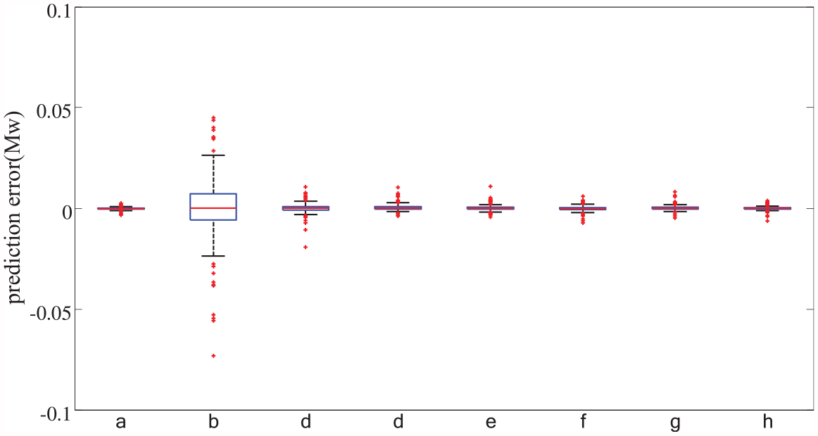
Box-plot of prediction errors comparison for data set B (a: proposed model; b: persistence model; c: ARIMA; d: GA-SVM; e: PSO-SVM; f: LSSVM; g: H-SVM; h: ELM).
From the comparison between the predicted value and the actual value, the comparison of the prediction error and its histogram distribution, the comparison of the performance indicators, the Pearson’s test results, DM test results and box-plot results all show that the prediction model proposed in this paper has better prediction accuracy and prediction effect than other comparison models.
Discussions
From the above comparison results, we can know that the proposed prediction model has achieved better results. According to obtained results from figures and tables, we can safely draw the conclusion that the proposed prediction model shows a more powerful forecasting ability than the comparison models. The main advantages of the proposed method in relation to compared models are as follows.
WD algorithm is introduced to pre-process wind power data. Wavelet denoising does not destroy the original characteristics of the wind power data, and the denoised data retains the peak of the original wind power data. Compared with the original wind power data, the capacity attenuation data after denoising is smoother. Wavelet denoising not only retains the authenticity of the original data to the greatest extent, but also removes the noise signal in the original wind power data. WD algorithm eliminates the adverse effect of noise and improves the prediction accuracy.
As a classical statistical learning model, SVM has the advantages of less samples and excellent regression performance. However, the performance of SVM is greatly affected by model parameters. In this study, the SMA algorithm is improved by using the random inertia weight mechanism. The SVM model parameters are optimized by ISMA, which further improves the performance of the prediction model.
Conclusions
In this study, SVM is applied to predict the wind power, which can accurately judge the future wind power data. However, because wind power is affected by many factors such as randomness, nonlinearity, and chaos, a lot of noise will affect the data modeling and prediction. Therefore, WD processing and SVM wind power prediction model are proposed, and ISMA algorithm is introduced into the optimization of SVM model parameters. Compared with other prediction models, the results show that the prediction results based on the proposed model are more in line with the actual value of wind power, effectively reduce the prediction error, and provide a novel modeling method for wind power prediction, which has stronger adaptability and high practical value.
The parameters of SVM are optimized by ISMA and used as the prediction model of wind power. However, there is still a need to improve the modeling accuracy and reduce the error. In order to meet the higher, faster, and more accurate prediction requirements, SMA can be further improved to better determine the best parameters of SVM model. On the other hand, how to determine a better and appropriate wavelet basis function to improve the noise reduction effect is also worthy of in-depth study.
Footnotes
Declaration of conflicting interests
The author(s) declared no potential conflicts of interest with respect to the research, authorship, and/or publication of this article.
Funding
The author(s) disclosed receipt of the following financial support for the research, authorship, and/or publication of this article: This work is partially supported by the Doctoral Scientific Research Foundation of Liaoning Province (Grant No. 20180540050).
Data availability statement
The data used to support the findings of this study are available from the corresponding author upon request.