Discrete wavelet transforms based hybrid approach to forecast wind speed time series

Abstract

The wind resources have been estimated by using physical models, statistical models, and artificial intelligence models. Wind power calculation helps us measure the annual energy that will sustain the balance between electricity generation and electricity consumption. Wind speed plays a significant role in calculating wind power, due to which here we focus on wind speed prediction. In this paper, hybrid models for wind speed forecasting have been proposed. The hybrid models are formed by combining the time series decomposition technique, that is, discrete wavelet transform (DWT), with statistical models, that is, autoregressive integrated moving average (ARIMA) and generalized autoregressive score (GAS), respectively. These hybrid models are referred to as DWT-ARIMA and DWT-GAS. DWT decomposes the original series into sub-series. After that, statistical models are applied to each sub-series for prediction. In the end, aggregate the prediction results of each sub-series to get the final forecasted series. For experimentation purposes, statistical and hybrid models are applied to various datasets that are taken from the NREL repository. In our studies, the hybrid version demonstrates better results in terms of accuracy and complexity, which indicates superior performance in most cases compared to the existing statistical models.

Keywords

ARIMA model GAS model DWT time series wind speed

Introduction

Wind energy is a renewable energy source; the demand is high as it is environmentally friendly and easily available in nature. Due to a renewable source, it is beneficial for economic development and environmental issues. It is also essential to manage wind energy on the trade-off for consumption (including establishment) and production. Research published in Morshedizadeh et al. (2017), Wadhvani and Shukla (2018), and Dongre and Pateriya (2019) concluded that there is a strong relationship between wind power and wind speed at the site. A useful wind speed prediction model can increase power forecasting accuracy. However, accurate wind speed forecasting for wind energy is an important task. It is challenging to get accurate predictive results due to the irregular wind speed behavior Liu et al. (2015). Wind speed forecasting is a type of time series prediction issue that provides valuable information that helps established wind power plants, scheduling, power distribution, and related activities Erdem and Shi (2011). There are currently several forecasting methods available, which can be classified into four classes: physical approach, statistical approach, artificial intelligence approach, and hybrid approach Lei et al. (2009). In the physical model, more complex variables are used; therefore, it takes more time to obtain the results, and it is generally considered for long-term predictions. It is mainly used by the numerical weather prediction models that establish a relationship between the factors affecting the wind speed forecasting and weather data such as temperature, pressure, altitude, and humidity Pelikán et al. (2010). Whereas, in statistical models, a relationship is maintained between the dependent and independent variables on the basis of historical data. Various statistical models are available, such as autoregressive (AR), moving average (MA), autoregressive moving average (ARMA) Yang et al. (2015), autoregressive integrated moving average (ARIMA) Torres et al. (2005), and generalized autoregressive score (GAS) Creal et al. (2013), which use past data to obtain the seasonal and trend components of wind time series data used for wind speed prediction. It is widely used in practice for getting the forecasting result because they are quick and straightforward. Besides, various factors impact the wind speed series and require a complex function to detect relationships between variables. Therefore they are not capable of handling the more complicated signal.

In recent years artificial intelligence models are frequently employed to develop the model for time series forecasting Barbounis and Theocharis (2007). These techniques include artificial neural network (ANN) Zhou et al. (2011), support vector machine (SVM) Pinto et al. (2014), and support vector regression (SVR) Santamaría-Bonfil et al. (2016). These models can maintain the relationship between the input and output data and have excellent error tolerance due to their outstanding performance in handling nonlinear and complicated signals Li and Shi (2010). The hybrid model is formed by combining the two or more above-mentioned models Xiao et al. (2016). Besides, an excellent hybrid model can only be obtained by the best combination of two or more different types of the model; the simple combination can result in a poor hybrid model. So, the structures of the hybrid model are essential Okumus and Dinler (2016). The above details indicate that a better-designed hybrid model can perform better than a randomly designed hybrid model Salcedo-Sanz et al. (2014). In recent years, various hybrid models are proposed for wind speed forecasting. Kushwah and Wadhvani (2019) have constructed a hybrid model by combining the GAS model and the neural network-based modeling techniques for wind speed forecasting on the 5-minute time interval. The results show that the hybrid model performs better as compared with the conventional statistical models. Shukur and Lee (2015) proposed the hybrid model, which is obtained by combining the Kalman Filter (KF) and the ANN models. In this model ARIMA model is also used to pick the KF’s preliminary parameters. The experimental results show that the hybrid version improves the accuracy of wind speed forecasting further. Cadenas and Rivera (2010) proposed a hybrid model based on the ARIMA version and ANN model. ARIMA model was first constructed here to forecast the wind speed and then produce the expected errors, which are given to the ANN models as an input. The results indicate that the hybrid version had better accuracy than the unbiased versions of ARIMA and ANN. Kushwah et al. (2020) suggested a hybrid model consisting of statistical models and trend-based clustering. Compared to statistical models used alone, the hybrid model performs better. Su et al. (2014) have proposed a hybrid model for wind speed prediction using particle swarm optimization (PSO), ARIMA, and KF. The PSO is used to refine the ARIMA version’s parameters, and the ARIMA variant is used to get the Kalman filter’s parameters. The experimental result showed that the hybrid model’s efficiency is better than that of ARIMA and ARIMA models optimized by PSO.

Another approach to handling the linear and nonlinear time series data is to use the time series decomposition techniques and apply the existing forecasting models. However, the decomposition-based prediction technique is a kind of hybrid approach that combines the various decomposition algorithms with forecasting models. Decomposition algorithms such as empirical mode decomposition Zhang et al. (2008), discrete wavelet transform Lei and Ran (2008), and ensemble empirical mode decomposition Wang et al. (2013) are generally used. There are many applications where hybrid models have performed better as compared to the different models used individually. Meng et al. (2016) have proposed a hybrid approach for forecasting time series by merging the wavelet packet decomposition and the artificial neural networks. The experimental results showed that the hybrid model performs better than the ANN alone. In this paper, a hybrid model for wind speed forecasting is proposed by combining the decomposition technique of discrete wavelet transform (DWT) with statistical models (ARIMA and GAS). This work proposed two hybrid models, namely, DWT-ARIMA and DWT-GAS. DWT is used to reduce the non-stationarity of wind time series data. DWT decomposes the original wind time series data into sub-series of low and high frequency. These sub-series are stationary as compared to the actual wind time series. The statistical model is applied to each sub-series and then aggregates each sub-series’ forecasting results to get the final forecasted series. The performance of statistical models and hybrid models are evaluated using the metrics Mean Absolute Error (MAE) and Root Mean Square Error (RMSE).

Statistical models for wind speed forecasting

This section describes the detail of statistical models used for wind speed forecasting. Wind speed is a type of time series forecasting problem which are used for wind power development. There are numerous statistical methods available for forecasting the wind time series, and the model ARIMA and GAS are commonly used.

ARIMA model

Ait Maatallah et al. (2015) have suggested the ARIMA model, which can represent different types of time series models such as the autoregressive (AR) model, the moving average (MA) model, and the ARMA model. These models have become very popular because of their flexibility and simplicity in representing the different time series. The ARIMA model is incorporated to handle the non-stationary time series data, whereas AR, MA, and ARMA models are used for stationary time series data. Here, the primary constraint is to assume the linear form of models that shows the direct connection structure for the time series data. ARIMA model can not capture the nonlinear pattern that is presented in the time-series data. The notation ARIMA (p; d; q) implies that the ARIMA model has p autoregressive terms, q moving-average terms, and d represents the differencing term’s degree. This model is described as:

y_{t} = α_{0} + α_{1} y_{t - 1} + \dots + α_{p} y_{t - p} + ε_{t} + β_{1} ε_{t - 1} + \dots + β_{q} ε_{t - q}

(1)

Where $y_{t}$ is a variable of interest. $α_{0}, α_{1}$ , …, $α_{p}$ are the AR coefficients, $β_{1}$ , …, $β_{q}$ are the MA coefficients, and $ε_{t}$ is assumed to be white noise.

GAS model

Creal et al. (2013) and Harvey (2013) have proposed the generalized autoregressive score (GAS) model, which is the new class of observation-driven model. The GAS model uses wind time series data to accommodate the varying density present in the time series data. A conditional observation density P $(y_{t} | θ_{t})$ describe the GAS model, where $y_{t}$ is the variable that to be forecasted, which depends on the time-varying parameter $θ_{t}$ . However, the word $θ_{t}$ is defined recursively by the autoregressive equation to update the time-varying parameter as:

θ_{t} = μ + \sum_{i = 1}^{p} ϕ_{i} θ_{t - i} + \sum_{j = 1}^{q} α_{j} S (θ_{j - 1}) \frac{\partial logp (y_{t - j} | θ_{t - j})}{\partial θ_{t - j}}

(2)

Where μ is a constant vector, ϕ is the coefficients of autoregressive terms, α represents the scaling parameter, s is the scaling factor which is multiplied with conditional observation density P. The scaling factor depending on $y_{t}$ and $θ_{t}$ . The GAS model’s essential contribution is the use of controlling mechanisms s, which are significant in some nonlinear models. Compared to the ARIMA model, the GAS model works best for nonlinear data. Since GAS relies on the score function, it only uses means and higher moments for the whole density structure.

Naive model

The Naive model is the most straightforward forecasting technique used in various data fields, such as economic and financial time series data Hyndman and Athanasopoulos (2018). This model assumes the data’s future value, which is equal to the last observed data value. This model is described as:

{\hat{y}}_{t + 1} = y_{t}

(3)

Where ${\hat{y}}_{t}$ is the forecasted variable, and $y_{t}$ is the variable of interest. The data’s prior knowledge is not required in this method, which serves as a benchmark for comparisons.

Time series decomposition

The original series of wind speed is decomposed into a collection of sub-series for better and more reliable behavior using the wavelet transform Percival and Walden (2000). Generally, there are two types of the wavelet transform, namely, continuous wavelet transform and discrete wavelet transform. An X(t) signal’s continuous wavelet transform (CWT) is shown as follows.

CW T_{x} (a, b) = \frac{1}{\sqrt{a}} \int_{- \infty}^{\infty} x (t) ψ (\frac{t - b}{a}) dt

(4)

Where a is the scale factor, b corresponds to the translation parameter and $ψ (\frac{t - b}{a})$ represents the mother wavelet. In this section, the unique time series is decomposed into sub-series by applying the discrete wavelet transform (DWT) technique. DWT is a broadly used mathematical approach that extracts patterns of statistical nature hidden in the original time series. It works by converting data into the corresponding frequency domain to detect the local trend and non-stationary pattern present in the time series data Aghajani et al. (2016). Using the dyadic scale and translation parameter, the CWT can be translated to DWT, which is defined as shown below.

DW T_{x} (p, q) = 2^{- (\frac{p}{2})} \sum_{t = 0}^{T - 1} x (t) ψ (\frac{t - q 2^{p}}{2^{p}})

(5)

Where t is the discrete-time index, T is the length of the given time series, a = $2^{p}$ is the discrete wavelet scaling factor and b = q $2^{p}$ is the parameter of the translation factor. Decomposing and reconstruction are the primary steps of the wavelet transform in data analysis Mallat (2009). The given series is decomposed in the decomposition process using the high pass and low pass filter. Compared to the original time series, the decomposed sub-series are classified as a detail component (called high-frequency components) and an approximation component (called low-frequency components). Filters decompose the approximation component further while the detail component remains unvaried. The procedure is repeated to a specified degree of decomposition. The subsequently produced detailed and approximation components are mixed in the reconstruction process to regenerate the original time series after forecasting. Figure 1 shows an X(t) signal DWT cycle with three decomposition stage.

Figure 1.

Wavelet Transform method with three decomposition levels: A is the approximate component, and D is the detail component.

Proposed hybrid approach for wind speed forecasting

The framework of the proposed hybrid model for wind speed forecasting is illustrated in Figure 2. The hybrid model is formed by combining the decomposition technique DWT and the following Statistical Models: ARIMA and GAS. First, DWT decomposes the original time series into a set of sub-series. These sub-series have both low frequency and high-frequency components, known as the approximation (A) and the detail components (D). These components are forecasted using ARIMA and GAS models, respectively. After predicting all the sub-series, forecasted results are aggregated to obtain the final wind speed forecasted data. The two-hybrid models are called the DWT-ARIMA and the DWT-GAS model. For the experimentation, the dataset is drawn from NREL’s wind prospector (National Renewable Energy Laboratory (NREL), 2012). The performance of proposed hybrid models is estimated using the criteria MAE and RMSE.

Figure 2.

The proposed hybrid (DWT-ARIMA/GAS) model.

Results and discussion

The full section describes the experiments carried out on different datasets and then examines the experiments’ results. The first section deals with the details of the datasets used for the experiment. Performance evaluation criteria are discussed in the second section. The third section analyses the results.

Dataset

In this section, we will explain the practical implementation of the modeling techniques described earlier. We use NREL sites such as 68003, 124693, 36363, 44402, 45208, 9687, 33423, 74664, 94404, and 72509. Among these sites, twenty datasets are obtained for our experiments. The geographical position of site id 68003 has −99.7579° longitude and 41.86517° latitudes. Table 1 includes a detailed overview of all datasets.

Table 1.

Dataset description.

Dataset	Site-Id	Year	Mean	Standard deviation	Min	Max
#1	68003	2011	8.021	3.553	0.094	28.974
#2	124693	2012	6.744	5.546	0.015	26.547
#3	36363	2012	8.120	3.826	0.036	29.590
#4	36363	2011	8.307	3.822	0.085	33.301
#5	36363	2010	8.234	3.783	0.048	24.875
#6	36363	2009	8.035	3.683	0.091	24.441
#7	36363	2008	8.481	3.921	0.018	31.625
#8	36363	2007	8.110	3.612	0.033	28.359
#9	44402	2012	5.649	4.272	0.029	24.103
#10	45208	2012	7.214	3.787	0.018	26.593
#11	9687	2012	5.933	4.294	0.018	27.774
#12	33423	2012	8.196	3.676	0.061	25.205
#13	33423	2011	8.589	3.752	0.048	25.879
#14	33423	2009	8.364	3.634	0.034	28.889
#15	33423	2008	8.647	3.787	0.055	27.209
#16	74664	2012	8.302	3.809	0.094	25.375
#17	94404	2012	8.464	5.411	0.055	31.647
#18	72509	2010	8.846	4.821	0.024	27.051
#19	72509	2009	9.186	5.187	0.045	34.119
#20	72509	2008	9.833	5.299	0.042	31.938

Performance measuring criteria

The performance of proposed hybrid models and existing statistical models are calculated using the required parameters to determine the models’ potential. Mean absolute error (MAE) and root mean squared error (RMSE) is used for our experiments to calculate the wind speed forecasting performance. The measurement parameters, such as MAE and RMSE, are further defined as:

MAE = \frac{1}{N} \sum_{i = 1}^{N} \hat{y} (i) - y (i)

(6)

RMSE = \sqrt{\frac{1}{N} \sum_{i = 1}^{N} {(\hat{y} (i) - y (i))}^{2}}

(7)

In this case, N is the cumulative number of observations, y indicate input variable and $\hat{y}$ represents the predicted variable. The minimum values of MAE and RMSE indicate the best-fitted model. The Python 3.6 version is used for the implementation of the ARIMA, GAS, and hybrid models.

Outlier detection in the dataset

There are several methods used for outlier detection in the dataset, such as boxplot, local outlier factor, etc. Boxplot is the most commonly used outlier detection method, which shows the distribution of numerical data of time series among with the minimum value, first quartile ( $Q_{1}$ ), second quartile ( $Q_{2}$ ), third quartile ( $Q_{3}$ ), and the maximum value Schwertman et al. (2004). The minimum (MIN) and maximum (MAX) values are defined as:

MIN = Q_{1} - 1.5 * IQR

(8)

MAX = Q_{3} + 1.5 * IQR

(9)

Where, $Q_{1}$ and $Q_{3}$ are the lower and upper range of the boxplot, $Q_{2}$ is the median of the boxplot. IQR represents the interquartile range, which is defined as:

IQR = Q_{3} - Q_{1}

(10)

Figure 3 shows the boxplot with outlier for dataset #2. Here the outliers are detected after the maximum value of the boxplot. After removing these outliers, our dataset is cleaned, which is shown in Figure 4.

Figure 3.

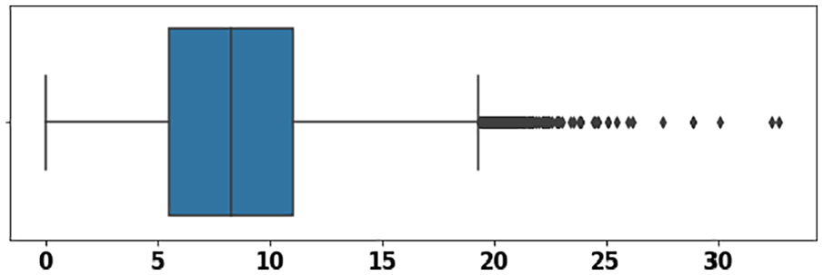
The boxplot with an outlier of wind time series data using dataset #2.

Figure 4.

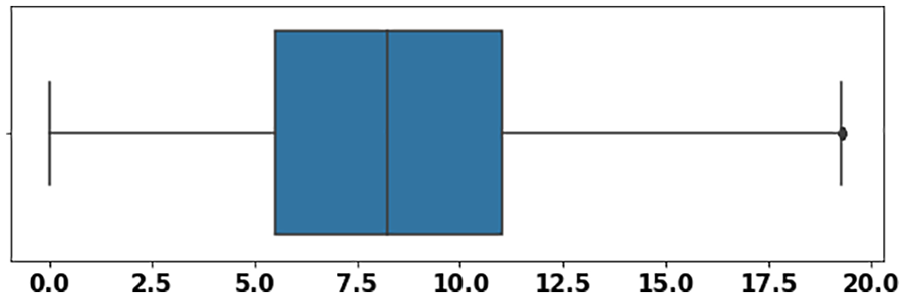
The boxplot after removal of the outlier of wind time series data using dataset #2.

Analysis of results

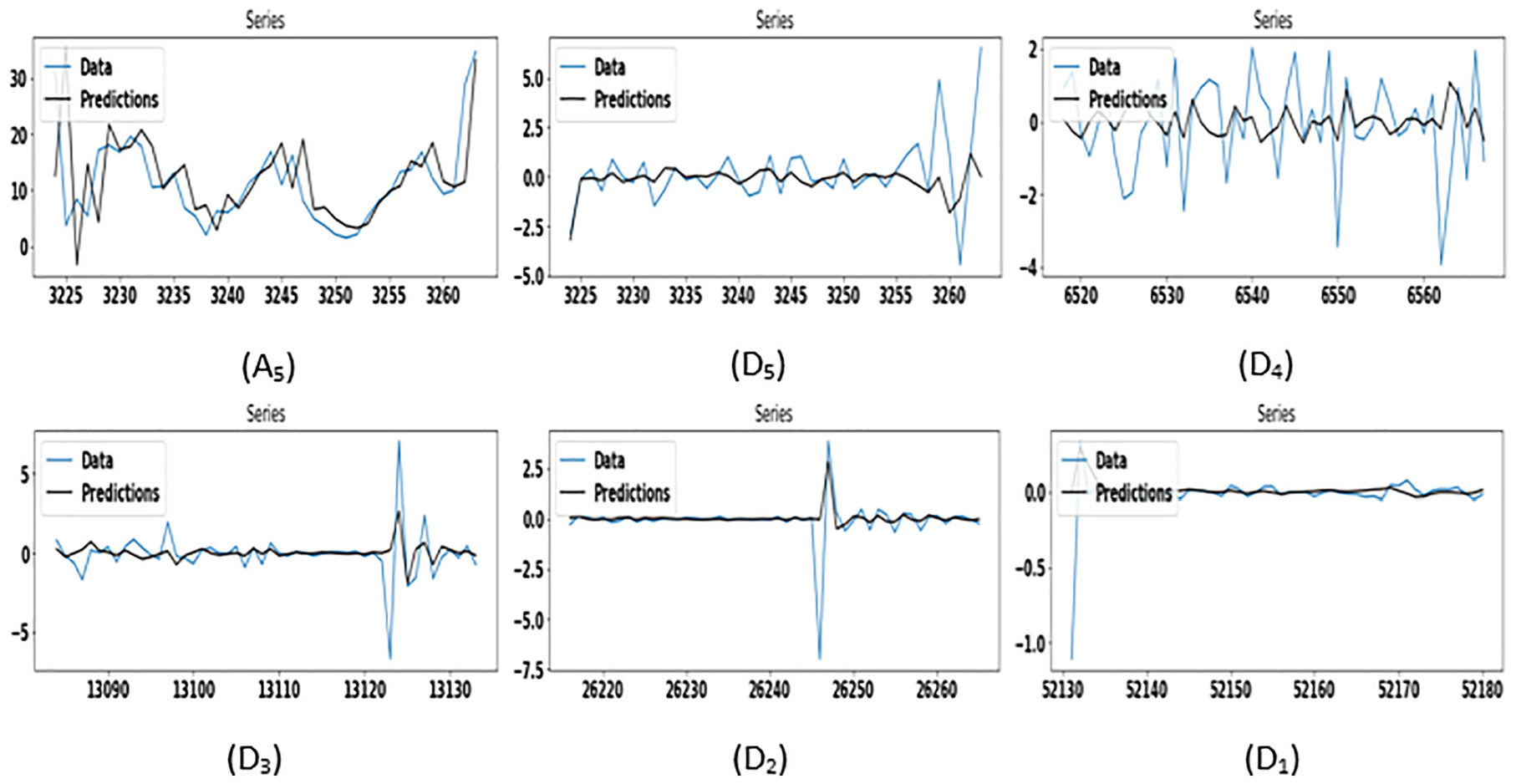
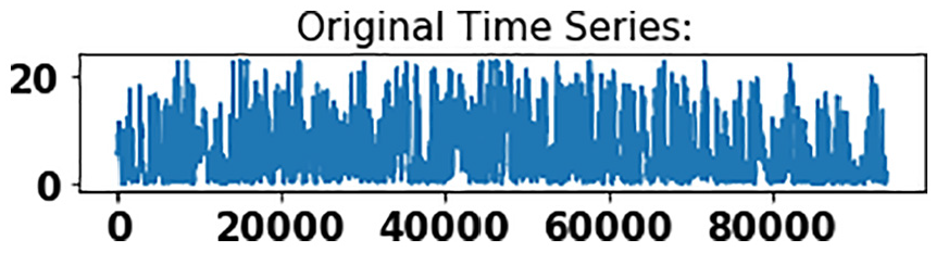
Statistical and the proposed hybrid models (ARIMA, GAS, DWT-ARIMA, and DWT-GAS) are applied for wind speed prediction on all the datasets. Figures 5 and 6 show the original and decomposed series. The original series is decomposed into sub-series using DWT with five decomposition label. Figure 4 shows one approximation component ( $A_{5}$ ) and five detailed components ( $D_{1}$ ; …; $D_{5}$ ). The approximation component shows the low frequency, and the detail components show the high-frequency components.

Figure 5.

Original wind speed time series.

Figure 6.

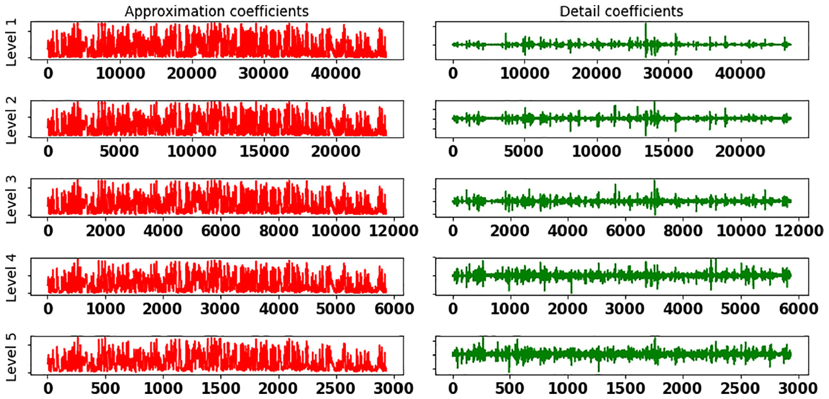
Wind speed time series decomposition using DWT with five labels.

The datasets used for experimentations are divided into training-testing pair. The training set contains 90% of the data, and the testing set contains 10% of the data. Figures 7 and 8 illustrate the wind speed prediction using ARIMA and GAS model applied separately on dataset #2. Here the GAS model shows better accuracy than the ARIMA model because the ARIMA model does not capture varying density present in this dataset, whereas the GAS model easily handles it and shows better accuracy.

Figure 7.

Wind speed prediction using the ARIMA model for dataset #2.

Figure 8.

Wind speed prediction using the GAS model for dataset #2.

The training results of all models in terms of MAE (maximum absolute error) and RMSE (root mean squared error) are shown in Table 2. In each row of the table, a “bold numeric value” of MAE and RMSE indicates that the prediction model corresponding to the column has the least prediction error and performed better on the Dataset representing that row.

Table 2.

Training Errors in terms of MAE, RMSE values of the proposed hybrid models compared with the existing methods.

Dataset	Naive		ARIMA		GAS		DWT-ARIMA		DWT-GAS
	MAE	RMSE	MAE	RMSE	MAE	RMSE	MAE	RMSE	MAE	RMSE
#1	0.292	0.541	0.249	0.281	0.189	0.365	0.136	0.232	0.115	0.205
#2	0.304	0.542	0.251	0.323	0.165	0.345	0.132	0.231	0.153	0.271
#3	0.319	0.572	0.519	0.622	0.245	0.387	0.435	0.534	0.122	0.229
#4	0.319	0.579	0.454	0.572	0.365	0.365	0.376	0.487	0.132	0.252
#5	0.303	0.535	0.657	0.801	0.265	0.401	0.459	0.562	0.121	0.205
#6	0.320	0.563	0.168	0.219	0.561	0.781	0.102	0.197	0.114	0.207
#7	0.334	0.594	0.473	0.594	0.287	0.354	0.398	0.451	0.167	0.299
#8	0.296	0.526	0.802	0.907	0.345	0.456	0.754	0.894	0.139	0.246
#9	0.275	0.490	0.887	0.889	0.354	0.487	0.365	0.462	0.123	0.211
#10	0.442	0.771	0.111	0.162	0.248	0.365	0.098	0.142	0.196	0.327
#11	0.342	0.617	0.697	0.719	0.257	0.348	0.465	0.612	0.138	0.269
#12	0.295	0.522	0.283	0.336	0.267	0.351	0.198	0.284	0.119	0.225
#13	0.297	0.525	0.631	0.745	0.298	0.305	0.523	0.672	0.128	0.248
#14	0.301	0.538	0.605	0.736	0.324	0.461	0.512	0.893	0.118	0.222
#15	0.308	0.557	0.342	0.423	0.365	0.421	0.298	0.334	0.152	0.281
#16	0.320	0.601	0.287	0.382	0.254	0.381	0.141	0.237	0.124	0.249
#17	0.260	0.444	0.520	0.662	0.365	0.468	0.454	0.528	0.271	0.568
#18	0.396	0.711	0.608	0.734	0.268	0.395	0.453	0.562	0.153	0.249
#19	0.429	0.782	0.427	0.508	0.241	0.345	0.384	0.469	0.137	0.235
#20	0.428	0.770	0.253	0.328	0.265	0.327	0.198	0.305	0.178	0.299

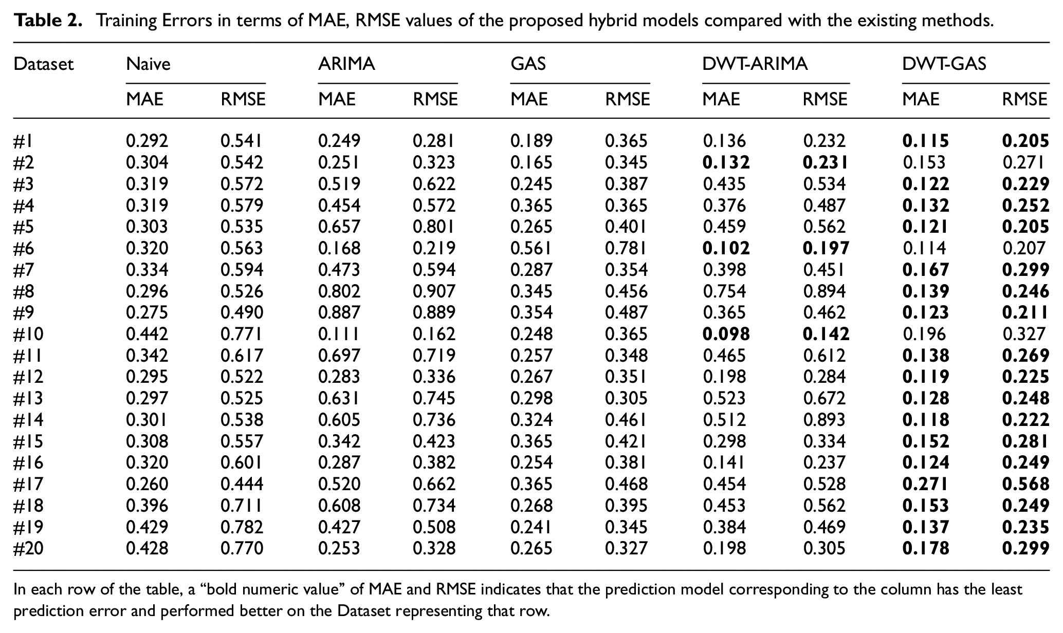
In each row of the table, a “bold numeric value” of MAE and RMSE indicates that the prediction model corresponding to the column has the least prediction error and performed better on the Dataset representing that row.

The testing results of all models in terms of MAE and RMSE values are given in Table 3. As shown in the table, the model DWT-ARIMA has minimum MAE and RMSE values compared to the ARIMA, GAS, and DWT-GAS models for series #1. For dataset #2, the model DWT-GAS has minimum MAE and RMSE values compared with the ARIMA, GAS, and DWT-ARIMA models. Therefore, it is concluded from our experimentations that the hybrid models perform superior to the existing ARIMA and GAS model.

Table 3.

Testing Errors in terms of MAE, RMSE values of the proposed hybrid models compared with the existing models.

Dataset	Naive		ARIMA		GAS		DWT-ARIMA		DWT-GAS
	MAE	RMSE	MAE	RMSE	MAE	RMSE	MAE	RMSE	MAE	RMSE
#1	4.597	5.339	3.632	4.452	3.132	3.768	3.086	3.663	3.082	3.623
#2	3.125	4.436	4.737	5.315	4.681	5.267	4.135	4.772	3.230	3.903
#3	4.462	5.393	3.575	4.254	3.456	4.123	3.227	3.899	3.012	3.521
#4	4.325	4.958	3.311	4.007	3.254	3.965	3.111	3.718	2.546	2.69
#5	3.559	4.627	3.664	4.401	3.548	4.215	3.337	3.976	2.481	3.152
#6	5.359	5.819	3.932	4.722	3.982	4.295	2.985	3.657	3.385	3.952
#7	3.609	4.682	3.711	4.499	3.854	4.178	3.625	4.392	3.154	3.781
#8	5.899	6.774	3.044	3.777	3.425	3.948	2.772	3.484	2.245	2.921
#9	4.461	4.921	5.668	6.307	4.982	5.824	3.822	4.316	4.182	4.876
#10	2.357	2.984	3.234	4.078	3.125	3.895	2.525	3.195	2.881	3.587
#11	2.981	3.536	5.118	5.697	4.652	5.231	3.525	4.132	3.346	3.991
#12	4.179	5.650	5.568	6.581	4.625	5.248	3.224	3.855	4.105	4.942
#13	3.312	4.125	3.469	4.169	3.125	4.215	3.439	4.129	2.625	3.417
#14	4.463	5.045	2.909	3.645	3.214	3.964	2.874	3.626	2.145	3.065
#15	4.114	5.056	3.603	4.365	3.524	4.025	3.513	4.211	2.198	3.127
#16	4.025	5.417	3.563	4.348	3.298	4.325	3.145	3.787	2.982	3.622
#17	2.762	3.514	5.080	5.970	4.685	4.958	4.769	5.784	3.856	4.253
#18	3.716	4.231	5.339	6.229	4.254	5.325	4.821	5.321	3.542	4.387
#19	4.686	5.589	7.034	8.515	5.684	6.025	3.365	4.240	4.846	5.922
#20	3.516	3.976	4.793	5.691	3.985	4.625	5.482	6.478	3.182	3.729

Note: The minimum values of MAE and RMSE for the prediction model are indicated in bold is referred as best performing model corresponding to the dataset representing that row.

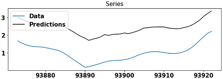
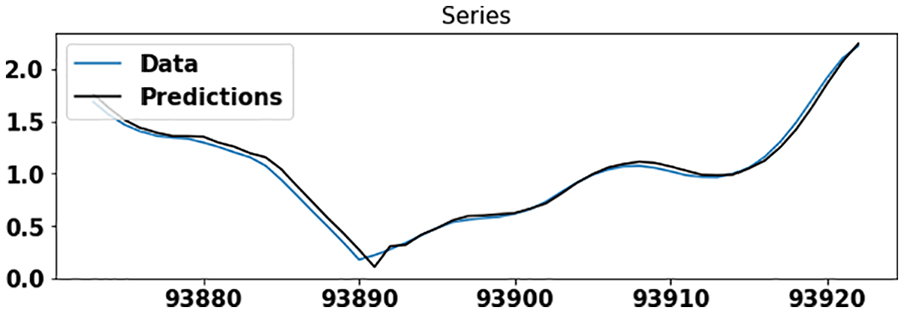
Figures 9 and 10 demonstrate the wind speed prediction using the DWT-ARIMA and DWT-GAS model, which is applied individually on each component of dataset #2. The DWT-GAS model shows better accuracy compared to the DWT-ARIMA model. Therefore, it can be concluded that $A_{5}$ is relatively complicated for prediction and may indicate the low prediction accuracy compared to $D_{5}$ , $D_{4}$ , $D_{3}$ , $D_{2}$ , and $D_{1}$ in a hybrid model (DWT-ARIMA and DWT-GAS).

Figure 9.

Wind speed prediction using the DWT-ARIMA model for dataset #2.

Figure 10.

Wind speed prediction using the DWT-GAS model for dataset #2.

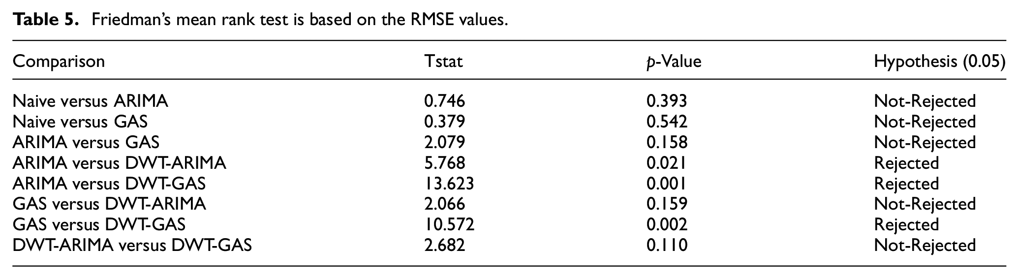
This research conducts the statistical t-test and Friedman’s mean rank test with a significance point of α = 0.05 on all the statistical models used for wind speed forecasting to evaluate the proposed model further. The statistical t-test results using MAE values calculated by statistical models have been shown in Table 4. The smaller p-value indicates a higher significant difference between the two models. The model ARIMA versus DWT-GAS has a more considerable difference in p-values relative to the other models. The Naive versus GAS model shows the least significant difference; hence, the null hypothesis is not rejected because of p-value > α. Similarly, Naive versus ARIMA, ARIMA versus GAS, GAS versus DWT-ARIMA, and DWT-ARIMA versus DWT-GAS show the least significant difference; hence the null hypothesis is not rejected. The statistical t-test results using the RMSE value are shown in Table 5. The ARIMA and DWT-GAS model has a more significant difference, whereas the Naive versus GAS model has the least significant difference in the p-value. Here, the null hypothesis for the models ARIMA versus DWT-ARIMA, ARIMA versus DWT-GAS, and GAS versus DWT-GAS are rejected.

Table 4.

Friedman’s mean rank test is based on the MAE values.

Comparison	Tstat	p-Value	Hypothesis (0.05)
Naive versus ARIMA	1.082	0.305	Not-Rejected
Naive versus GAS	0.007	0.929	Not-Rejected
ARIMA versus GAS	1.053	0.311	Not-Rejected
ARIMA versus DWT-ARIMA	5.379	0.026	Rejected
ARIMA versus DWT-GAS	13.549	0.001	Rejected
GAS versus DWT-ARIMA	2.747	0.106	Not-Rejected
GAS versus DWT-GAS	11.585	0.001	Rejected
DWT-ARIMA versus DWT-GAS	2.862	0.099	Not-Rejected

Table 5.

Friedman’s mean rank test is based on the RMSE values.

Comparison	Tstat	p-Value	Hypothesis (0.05)
Naive versus ARIMA	0.746	0.393	Not-Rejected
Naive versus GAS	0.379	0.542	Not-Rejected
ARIMA versus GAS	2.079	0.158	Not-Rejected
ARIMA versus DWT-ARIMA	5.768	0.021	Rejected
ARIMA versus DWT-GAS	13.623	0.001	Rejected
GAS versus DWT-ARIMA	2.066	0.159	Not-Rejected
GAS versus DWT-GAS	10.572	0.002	Rejected
DWT-ARIMA versus DWT-GAS	2.682	0.110	Not-Rejected

The proposed hybrid approach based on the GAS model and DWT techniques (DWT-GAS) has the least mean-ranks in the Friedman test, shown in Figures 11 and 12, respectively. The Friedman test computes the rank of each model on the 20 datasets. In our experimentation, the DWT-ARIMA and DWT-GAS models outperform the ARIMA and the GAS models, respectively.

Figure 11.

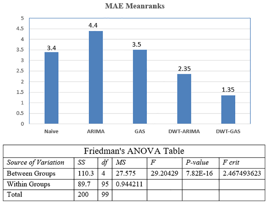
Friedman’s mean ranks and ANOVA table for MAE with α = 0.05.

Figure 12.

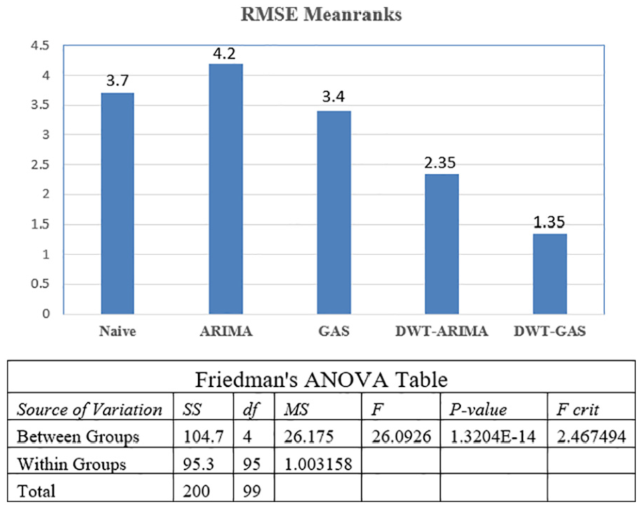
Friedman’s mean ranks and ANOVA table for RMSE with α = 0.05.

Conclusions

The present work focuses on selecting the best suitable modeling approach to wind speed forecasting. This study has proposed the hybrid models and applied the existing statistical models to predict the wind speed time series on 20 different datasets. For each dataset in the proposed hybrid approaches, the DWT technique is used to decompose the original series into a set of sub-series. Then the ARIMA and GAS model is applied to each sub-series. These sub-series are relatively stationary as compared to the original series. Finally, predicted wind speed is aggregated to get the overall predicted series. In our experiments, the hybrid model performs better as compared to the existing Naive, ARIMA, and GAS models. The wind speed series data has both high-frequency variants and low-frequency variants, which depict long-time period trends. The ARIMA and GAS models are not effective in capturing all the detail in wind speed data. The hybrid approaches take care of both the high-frequency variants and the low-frequency variants in wind speed series data, making it a powerful forecasting technique. In the future, advanced neural network-based approaches for sequential modeling along with decomposition techniques can be applied to achieve higher accuracy.

Footnotes

Declaration of conflicting interests

The author(s) declared no potential conflicts of interest with respect to the research, authorship, and/or publication of this article.

Funding

The author(s) received no financial support for the research, authorship, and/or publication of this article.

ORCID iD

Anil Kumar Kushwah

References

Aghajani

Kazemzadeh

Ebrahimi

(2016) A novel hybrid approach for predicting wind farm power production based on wavelet transform, hybrid neural networks, and imperialist competitive algorithm. Energy Conversion and Management 21: 232–240.

Ait Maatallah

Achuthan

Janoyan

, et al. (2015) Recursive wind speed forecasting based on Hammerstein Auto-Regressive model. Applied Energy 145: 191–197.

Barbounis

Theocharis

(2007) Locally recurrent neural networks for wind speed prediction using spatial correlation. Information Science 177: 5775–5797.

Cadenas

Rivera

(2010) Wind speed forecasting in three different regions of Mexico, using a hybrid ARIMA-ANN model. Renewable Energy 35: 2732–2738.

Creal

Koopman

Lucas

(2013) Generalized autoregressive score models with applications. Journal of Applied Econometrics 28(5): 777–795.

Dongre

Pateriya

(2019) Power curve model classification to estimate wind turbine power output. Wind Engineering 43(3): 213–224.

Erdem

Shi

(2011) ARMA based approaches for forecasting the tuple of wind speed and direction. Applied Energy 88: 1405–1414.

Harvey

(2013) Dynamic Models for Volatility and Heavy Tails: With Applications to Financial and Economic Time Series. New York, NY: Cambridge University Press.

Hyndman

Athanasopoulos

(2018) Forecasting: Principles and Practice, 2nd edn. Melbourne, Australia: OTexts. Available at: OTexts.Com/fpp2 (accessed 25 September 2020).

10.

Kushwah

Wadhvani

(2019) Performance monitoring of wind turbines using advanced statistical methods. Sadhana 44: 163.

11.

Kushwah

Wadhvani

Kushwah

(2020) Trend based time series data clustering for wind speed forecasting. Wind Engineering. Epub ahead of print 21 July 2020. DOI: 10.1177/0309524X20941180.

12.

Lei

Ran

(2008) Short-term wind speed forecasting model for the wind farm based on wavelet decomposition. In: 2008 third international conference on electric utility deregulation and restructuring and power technologies, Nanjing, China, 6–9 April 2008, pp.2525–2529. New York: IEEE.

13.

Lei

Shiyan

Chuanwen

, et al. (2009) A review on the forecasting of wind speed and generated power. Renewable and Sustainable Energy Reviews 13(4): 915–920.

14.

Shi

(2010) On comparing three artificial neural networks for wind speed forecasting. Applied Energy 87: 2313–2320.

15.

Liu

Tian

, et al. (2015) Comparison of four Adaboost algorithm based artificial neural networks in wind speed predictions. Energy Conversion and Management 92: 67–81.

16.

Mallat

(2009) A theory for multiresolution signal decomposition: The wavelet representation. Fundamental Papers in Wavelet Theory 2: 494–513.

17.

Meng

Yin

, et al. (2016) Wind speed forecasting based on wavelet packet decomposition and artificial neural networks trained by crisscross optimization algorithm. Energy Conversion and Management 114: 75–88.

18.

Morshedizadeh

Kordestani

Carriveau

, et al. (2017) Improved power curve monitoring of wind turbines. Wind Engineering 41(4): 260–271.

19.

National Renewable Energy Laboratory (NREL) (2012) Western dataset (Site-id 124693). Available at: https://www.nrel.gov/grid/western-wind-data.html.

20.

Okumus

Dinler

(2016) Current status of wind energy forecasting and a hybrid method for hourly predictions. Energy Conversion and Management 123: 362–371.

21.

Pelikán

Eben

Resler

, et al. (2010) Wind power forecasting by an empirical model using NWP outputs. In: 2010 9th international conference on environment and electrical engineering, Prague, Czech Republic, 16–19 May 2010, pp.45–48. New York: IEEE.

22.

Percival

Walden

(2000) Wavelet Methods for Time Series Analysis. Wavelet Methods Time Series. New York, NY: Cambridge University Press.

23.

Pinto

Ramos

Sousa

, et al. (2014) Short-term wind speed forecasting using Support Vector Machines. In: IEEE symposium series on computational intelligence in dynamic and uncertain environments (CIDUE), Orlando, FL, 9–12 December 2014, pp.40–46. New York: IEEE.

24.

Salcedo-Sanz

Pastor-Sánchez

Prieto

, et al. (2014) Feature selection in wind speed prediction systems based on a hybrid coral reefs optimization - Extreme learning machine approach. Energy Conversion and Management 87: 10–18.

25.

Santamaría-Bonfil

Reyes-Ballesteros

Gershenson

(2016) Wind speed forecasting for wind farms: A method based on support vector regression. Renewable Energy 85: 790–809.

26.

Schwertman

Owens

Adnan

(2004) A simple more general boxplot method for identifying outliers. Computational Statics and Data Analysis 47: 165–174.

27.

Shukur

Lee

(2015) Daily wind speed forecasting through hybrid KF-ANN model based on ARIMA. Renewable Energy 76: 637–647.

28.

Wang

, et al. (2014) A new hybrid model optimized by an intelligent optimization algorithm for wind speed forecasting. Energy Conversion and Management 85: 443–452.

29.

Torres

García

De Blas

, et al. (2005) Forecast of hourly average wind speed with ARMA models in Navarre (Spain). Solar Energy 79(1): 65–77.

30.

Wadhvani

Shukla

(2018) Analysis of parametric and non-parametric regression techniques to model the wind turbine power curve. Wind Engineering 43(3): 225–232.

31.

Wang

Zhang

(2013) A novel wind speed forecasting method based on ensemble empirical mode decomposition, and GA-BP neural network. In: 2013 IEEE power & energy society general meeting, Vancouver, BC, Canada, 21–25 July 2013, pp.1–5. New York: IEEE.

32.

Xiao

Shao

Wang

, et al. (2016) Research and application of a hybrid model based on multi-objective optimization for electrical load forecasting. Applied Energy 180: 213–233.

33.

Yang

Sharma

, et al. (2015) Forecasting of global horizontal irradiance by exponential smoothing, using decompositions. Energy 81: 111–119.

34.

Zhang

Lai

Wang

(2008) A new approach for crude oil price analysis based on Empirical Mode Decomposition. Energy Economics 30: 905–918.

35.

Zhou

Shi

(2011) Fine tuning support vector machines for short-term wind speed forecasting. Energy Conversion and Management 52: 1990–1998.