A STL decomposition-based deep neural networks for offshore wind speed forecasting

Abstract

Accurate prediction of offshore wind speed is of great significance for optimizing operation strategies of offshore wind power. Here, a novel hybrid algorithm based on seasonal-trend decomposition with loess (STL) and auto-regressive integrated moving average (ARIMA)- long short-term memory neural network (LSTM) is proposed to eliminate seasonal factors in wind speed and fully exert the advantages of ARIMA processing linear series and LSTM processing nonlinear series. Moreover, wind speed are comprehensively preprocessed and statistically analyzed. Then, we handle information leakage problem. Finally, STL-ARIMA-LSTM model is applied to wind speed forecasting on 3 time-scales. The proposed model has the highest accuracy and resolution for the trend and periodicity of wind speed, and the lag problem of very shortterm wind speed prediction can be solved. This study also shows that when predicting offshore wind speed, we can handle the strong intermittence, volatility and outliers in wind speed by gradually adjusting time scale.

Keywords

Offshore wind wind speed prediction ARIMA LSTM STL decomposition hybrid model

Introduction

The development of wind power can protect the ecological environment, improve the energy structure and achieve sustainable economic growth (Afshar et al., 2018). Compared with onshore wind power generation, offshore wind energy resources are more stable, wind turbine utilization is higher, and does not occupy land resources. However, the uncertainty, intermittence and volatility of offshore wind (Boutoubat et al., 2013) not only challenges the security of power system, but also poses a great challenge to the accurate forecasting of wind speed. Consequently, the accurate prediction of wind speed is an indispensable prerequisite for planning wind farms and dispatching power grids. In recent years, the statistical method and the machine learning method have been widely concerned and developed in the field of wind energy prediction.

In statistical methods, autoregressive moving average model (ARMA) and ARIMA are suitable for predicting very shortterm or shortterm wind speed. ARMA is utilized to calculate hourly mean wind speed at five locations in Spain (Torres et al., 2005). Even if the model is simple, they also obtained good prediction results. Erdem and Shi (2011) studied the performance of ARMA in wind speed and direction prediction for hourly mean wind by comparing vector autoregression (VAR) model. Their results showed that ARMA has good advantages in wind speed forecasting, and VAR can enhance the accuracy of wind direction prediction. ARIMA model (Box and Jenkins, 1970) was established by adding d-order difference process on the basis of ARMA model, which can make the calculation of time series more stable in theory. ARIMA model has been used in many time-series forecasting tasks because of its simple calculation, which is also popular in wind speed time series prediction (Benth and Benth, 2010; Cadenas and Rivera, 2010; Kavasseri and Seetharaman, 2009). Wind has high-frequency oscillation and seasonality, whereas ARIMA has the advantage of processing linear series. Therefore, we may first decompose the sequence, and then the decomposed components are modeled by ARIMA. For instance, Aasim et al. (2019) applied ARIMA with repeated wavelet transform (RWT) decomposition to very shortterm wind speed forecasting and studied the superiority of ARIMA with RWT decomposition by comparing with WT decomposition. Alternatively, considering that wind speed has linear trend and nonlinear trend, the linear trend component can be modeled by ARIMA, and the nonlinear part can be modeled by other suitable algorithms. Some machine learning models show their superior performance in dealing with nonlinear wind speed prediction problems.

The representative machine learning model includes random forest (RF; Lin et al., 2015), support vector machine (SVM; Mohandes et al., 2004), artificial neural network (ANN; Hur, 2021; Shboul et al., 2021), convolutional neural network (CNN; Wang et al., 2017, 2020b), deep belief network (DBN; Khodayar et al., 2019; Zhang et al., 2020), recurrent neural network (RNN) and so on. As a variant of RNN, LSTM neural network has advantages in terms of time series prediction and has made some progress in wind speed forecasting (Chen et al., 2019; Qin et al., 2019; Wang et al., 2020a). However, a single model is not competent to accurately predict complex wind speed time series. As a result, a complex time series can be decomposed into different components, combined with the advantages of each model to make predictions, which will usually achieve better prediction results than a single model (Olaofe and Folly, 2012). In recent years, some signal-decomposition methods such as wavelet packet decomposition (WPD; Liu et al., 2020), empirical mode decomposition (EMD) and variational mode decomposition (VMD) have been integrated into the hybrid model to preprocess the original wind speed signals. In addition, Wen et al. (2019) decomposed the wind speed time series by using STL and analyzed the potential characteristics of wind speed. STL decomposition method developed by Cleveland and Cleveland (1990) is a filtered seasonal decomposition method, which is simple and flexible. A few outliers do not affect the estimation of trend period and seasonal factors when processing time series data. Therefore, the paper will adopt STL method to adjust the seasonal wind speed time series.

LSTM neural network has wonderful feature in handling nonlinear wind speed due to its great ability to handle longterm correlation problem (Liu et al., 2018a, 2018b; Wang and Hu, 2015). Memarzadeh and Keynia (2020) developed a hybrid model with LSTM, which combined CSA, WT, FS and MI. Their model was used to predict wind speed and proved to be reliable. Chen et al. (2018) presented EnsemLSTM, and based on the model, the nonlinear feature of shortterm wind series was well captured. Jaseena and Kovoor (2021) applied hybrid BiDLSTM to predict wind speed, and achieved good prediction result.

Meanwhile, if the signal decomposition method is adopted in the process of wind speed prediction, the information leakage (Qian et al., 2019) is noteworthy. We can find a phenomenon that, if we normalize the data first and then divide train set and test set, high-precision results can be achieved based on the prediction model, but when this high-precision prediction method is applied to the actual working condition, its accuracy is often greatly reduced or the calculation results are incorrect. If the whole data set is decomposed first then substituted into the model to predict, the above result will also be obtained. These phenomena are the result of information leakage. Actually, the model training stage involves “future” data that should be unknown, which leads to information leakage. In this paper, we will deal with the problem of information leakage.

In this paper, combining the advantages that ARIMA model is easier to capture the linear relationship in the sequence and LSTM is easier to capture the nonlinear relationship in the sequence, a novel ARIMA-LSTM multi-scale hybrid model based on STL seasonal adjustment is proposed for wind speed time series prediction. The reason for choosing this hybrid model is that, in fact, the single ARIMA is hard to attain the accuracy results in forecasting non-linear and non-stationary time series, while the single LSTM model has the problem of forecasting lag, whereas seasonal factors in wind speed time series can not be ignored. Therefore, we first preprocess the original data, and then eliminate the seasonal factors in the data by STL decomposition. The processed data are predicted by ARIMA model to obtain the prediction results and residual values, and the residual value is predicted by LSTM. Finally, the predicted value of ARIMA is combined with the predicted value of LSTM to obtain the final prediction result. Moreover, in order to better satisfy the requirement of the actual project, multi-scale analysis of wind speed series is carried out, and original wind speed time series is divided into 3 time scales containing hour, day and month. In addition, STL decomposition of time series and data normalization preprocessing also avoid information leakage and ensure the forecasting accuracy. The main contributions of this paper are summarized as follows.

(1) In this paper, a detailed selection analysis experiment is carried out on the sample data of offshore wind speed and the problem of information leakage is fully considered, which can provide reliable prediction results;

(2) Compared with other decomposition methods, STL decomposition has better interpretability. Therefore, this paper uses STL decomposition method to extract the seasonal features in the sequence. Such feature extraction is convenient for the prediction of subsequent models, and the seasonal factors of wind speed can also be fully considered;

(3) ARIMA model can capture the linear relationship in the data, and LSTM model can capture the nonlinear relationship in the data. We use the hybrid method of ARIMA and LSTM to predict the seasonally processed data. This model is to use the prediction error to make a small linear correction to the wind speed value of the nonlinear prediction of the neural network. Therefore, the proposed model can effectively solve the lag problem in very shortterm wind speed prediction and improve the accuracy of predicting multiple time scale data;

(4) The proposed model shows the best performance and is reliable under the verification of three types of data and the comparison of multiple models. In addition, the prediction results of three different time scales of wind speed series also point out the direction for our future research.

Wind speed series preprocessing

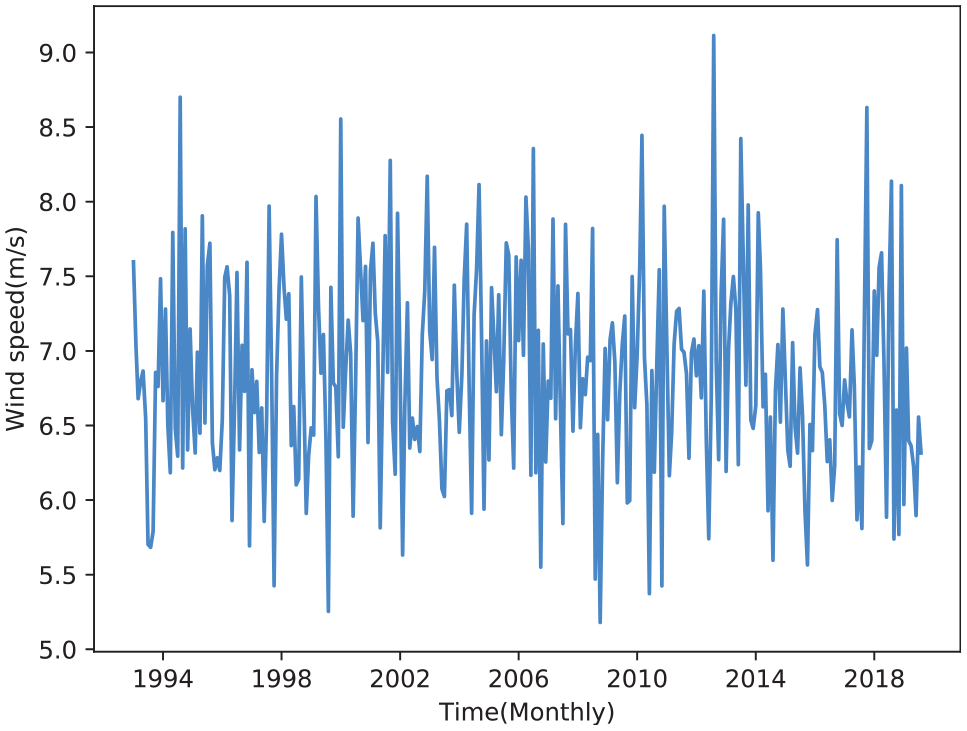
Wind speed has the characteristics of intermittent, randomness and volatility, as well as the characteristics of data loss and data redundancy caused by the acquisition process, particularly offshore wind speed, which directly leads to the time-consuming data processing and analysis and the inability to extract useful information. This paper chooses the offshore wind speed data with a sampling interval of 1 hour and a height of 50 m in Nanhui District of Shanghai from 1993 to 2019 as the research object. The visualization of time series data can provide valuable diagnosis for determining wind speed trend and seasonal variation. Figure 1 shows a box plot where maximum and minimum values, median value, upper and lower quartile values can be clearly observed. Figure 2 illustrates the wind speed distribution curve with time. In order to accurately and fully mine the data information, it is necessary to preprocess and statistically analyze the wind speed series.

Figure 1.

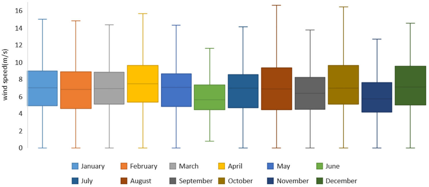
Box plot of wind speed time sequences.

Figure 2.

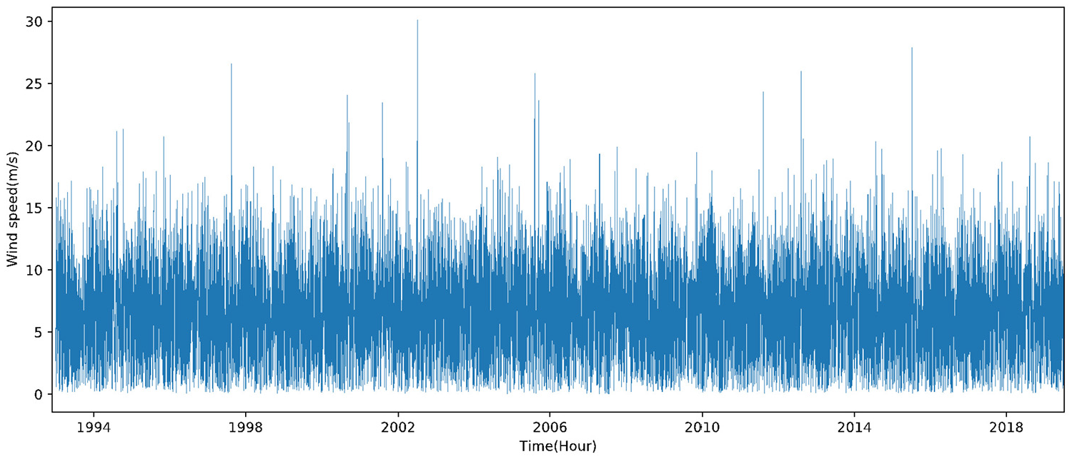
Line plot of wind speed time sequences.

Missing value and downsampling processing

First, we handle the missing values in the wind speed time series that are numeric types. Considering the missing value ratio is small and the data structure is relatively standard, the missing value is solved by using linear interpolation on its two nearest neighbors.

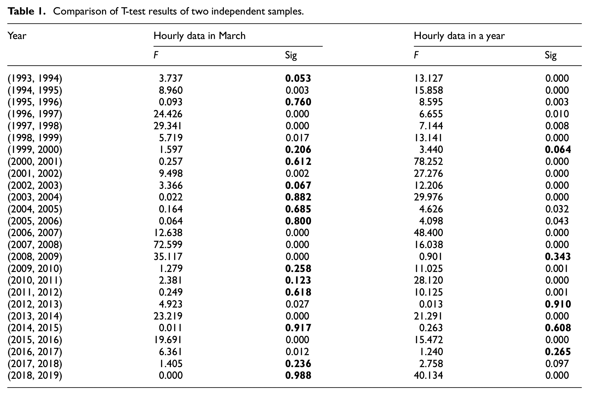
The prediction accuracy is related to the time scale of wind speed. For comprehensively investigate the proposed model, we downsample the raw wind speed sequence and converted it from high frequency sequence to the low frequency sequence, and divide it into three sub sample time series with different time scales, namely very shortterm, shortterm and longterm time series. For the very shortterm sub-sample series, we select the hourly data in March each year to calculate. In fact, affected by seasons, the annual wind speed series has strong nonlinearity, whereas the nonlinearity for the data over a short time such as a month would become weak. Here, considering the large amount of data, we adopt independent T-test method in Statistical Hypothesis Testing to test the data distribution differences between 2 adjacent years and 2 months corresponding to adjacent years respectively. The statistically significant level $α$ is taken as $0.05$ commonly used in statistical analysis. If Sig is less than $α$ , it can be considered that there is significant difference between two groups.

Table 1 shows the T-test results of hourly dataset in March and hourly dataset in 1 year. The bold values in the table indicate that their Sig value is greater than 0.05. For the case of 1 year, the results with significant difference (Sig <0.05) are up to about 81% which is much bigger than the results of the case of March, which implies the distribution difference of hourly wind speed in March is smaller than that of a whole year. Therefore, for very shortterm time series, it is feasible to select the historical wind speed data in March rather than the data in 1 year for wind resource prediction.

Table 1.

Comparison of T-test results of two independent samples.

Year	Hourly data in March		Hourly data in a year
	F	Sig	F	Sig
(1993, 1994)	3.737	0.053	13.127	0.000
(1994, 1995)	8.960	0.003	15.858	0.000
(1995, 1996)	0.093	0.760	8.595	0.003
(1996, 1997)	24.426	0.000	6.655	0.010
(1997, 1998)	29.341	0.000	7.144	0.008
(1998, 1999)	5.719	0.017	13.141	0.000
(1999, 2000)	1.597	0.206	3.440	0.064
(2000, 2001)	0.257	0.612	78.252	0.000
(2001, 2002)	9.498	0.002	27.276	0.000
(2002, 2003)	3.366	0.067	12.206	0.000
(2003, 2004)	0.022	0.882	29.976	0.000
(2004, 2005)	0.164	0.685	4.626	0.032
(2005, 2006)	0.064	0.800	4.098	0.043
(2006, 2007)	12.638	0.000	48.400	0.000
(2007, 2008)	72.599	0.000	16.038	0.000
(2008, 2009)	35.117	0.000	0.901	0.343
(2009, 2010)	1.279	0.258	11.025	0.001
(2010, 2011)	2.381	0.123	28.120	0.000
(2011, 2012)	0.249	0.618	10.125	0.001
(2012, 2013)	4.923	0.027	0.013	0.910
(2013, 2014)	23.219	0.000	21.291	0.000
(2014, 2015)	0.011	0.917	0.263	0.608
(2015, 2016)	19.691	0.000	15.472	0.000
(2016, 2017)	6.361	0.012	1.240	0.265
(2017, 2018)	1.405	0.236	2.758	0.097
(2018, 2019)	0.000	0.988	40.134	0.000

Data descriptive statistics

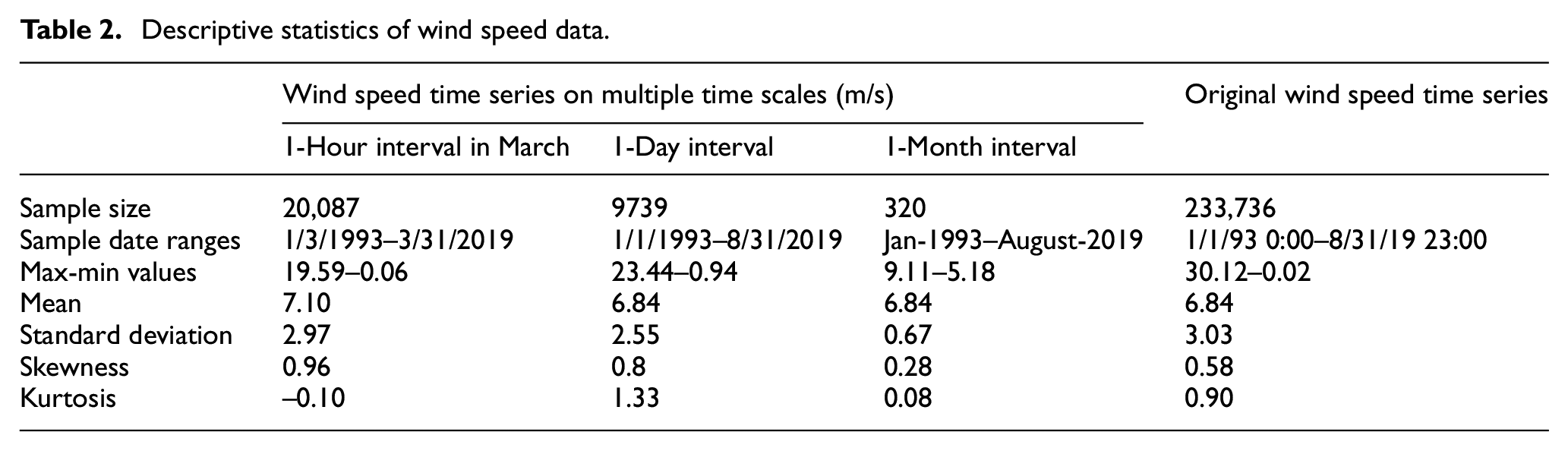
Here, we briefly give descriptive statistics of data on 3 time scales involving hours, days and months, in order to have an intuitive understanding of the samples to be studied. Table 2 shows the sample size, maximum / minimum value, expectation, root variance, coefficients of skewness and kurtosis of the 3 time scale data. It can be observed that three coefficients of skewness are positive, which indicates that their distribution patterns are all positive partial peaks. The coefficient of kurtosis of 1-hour interval in March is −0.10, which represents the peak of data distribution is wider than that of Gauss distribution. The coefficients of kurtosis of 1-day interval and 1-month interval are positive, which represents the peaks of data distribution are steeper than that of Gauss distribution. The standard deviation of hourly time scale series is the largest, followed by daily time scale series, which further shows that the wind speed time series has strong volatility.

Table 2.

Descriptive statistics of wind speed data.

	Wind speed time series on multiple time scales (m/s)			Original wind speed time series
	1-Hour interval in March	1-Day interval	1-Month interval
Sample size	20,087	9739	320	233,736
Sample date ranges	1/3/1993–3/31/2019	1/1/1993–8/31/2019	Jan-1993–August-2019	1/1/93 0:00–8/31/19 23:00
Max-min values	19.59–0.06	23.44–0.94	9.11–5.18	30.12–0.02
Mean	7.10	6.84	6.84	6.84
Standard deviation	2.97	2.55	0.67	3.03
Skewness	0.96	0.8	0.28	0.58
Kurtosis	–0.10	1.33	0.08	0.90

Data normalization processing

For eliminating the influence of different ranges of the samples on the prediction accuracy, facilitate data processing and ensure faster convergence when the program runs. The data needs dimensionless normalization, which can be realized by linear mapping to the interval [0,1]

x = \frac{x_{t} - x_{\min}}{x_{\max} - x_{\min}} .

(1)

If the entire dataset is directly normalized, and then one part constitutes training set and the rest is test set, it is obvious that the data information in the training set will be leaked to the test set, which will lead to the problem of information leakage (Qian et al., 2019; Wang and Wu, 2016). This kind of information leakage will cause an illusion that the mathematical model has high accuracy.

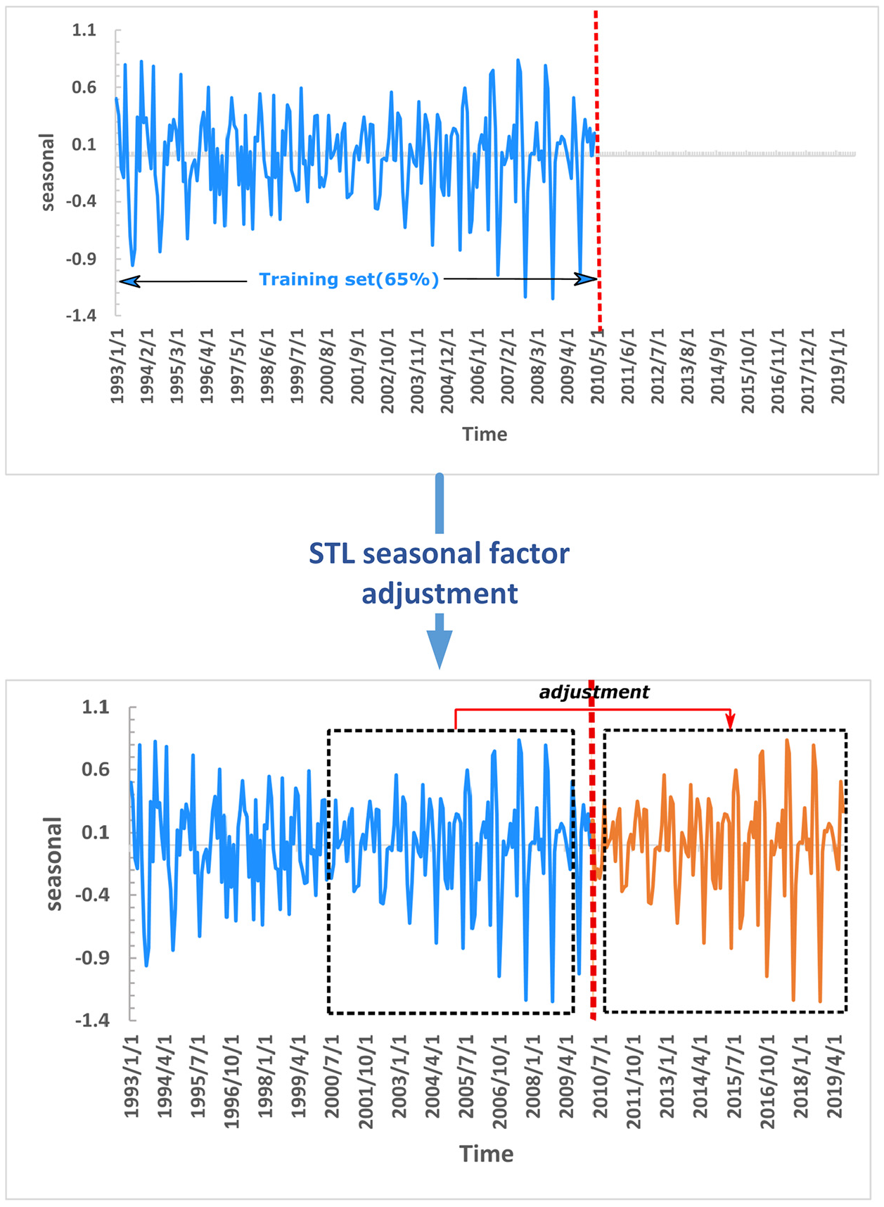
In order to avoid the problem of data information leakage, as shown in Figure 3, the normalization of training set and test set is processed separately, where the training set accounts for 65% and the test set accounts for 35%.

Figure 3.

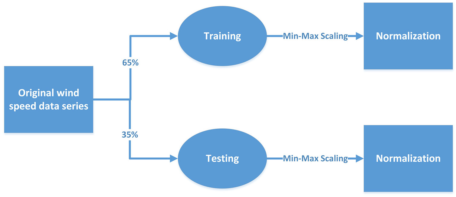
Separate normalization to avoid information leakage.

Processing of data stationarity

Time series can be classified into stationary and non-stationary sequences. Stationary sequence doesn’t basically include trend, in which trend refers to the law that the time series shows a continuous rise or decline over a long period of time, including linear trend and nonlinear trend. Specifically, if the values of mean, variance and covariance or self variance of sample time series do not change with time, which can also be considered to remain unchanged in the future, then the sample time series is called a stationary time series. Generally, we can transform non-stationary sequence into a stationary sequence with difference method.

In the paper, the unit root ADF test method (Krämer, 1998) is adopted to check the stationarity. Table 3 shows the ADF test results of multi-time scale wind speed time series. It can be concluded from the table that only the p-value of monthly time scale sequence is greater than 0.05, which indicates that this time series is non-stationary. Because ARIMA is good at handling stationarity time series, a difference operation is performed as follows

Δ X_{t} = X_{t} - X_{t - 1} = (1 - L) X_{t}

(2)

Table 3.

Results of ADF test on multiple time scale.

Augmented Dickey-Fuller test statistics		t-statistic	p-Value
Augmented Dickey-Fuller test statistics (hourly data in March)		–15.15	6.75E–28
Critical value	1%level	–3.43
	5%level	–2.86
	10%level	–2.57
Augmented Dickey-Fuller test statistics (daily data)		–12.71	1.05E–23
Critical value	1%level	–3.43
	5%level	–2.86
	10%level	–2.57
Augmented Dickey-Fuller test statistics (monthly data)		–2.51	0.11
Critical value	1%level	–3.43
	5%level	–2.86
	10%level	–2.57

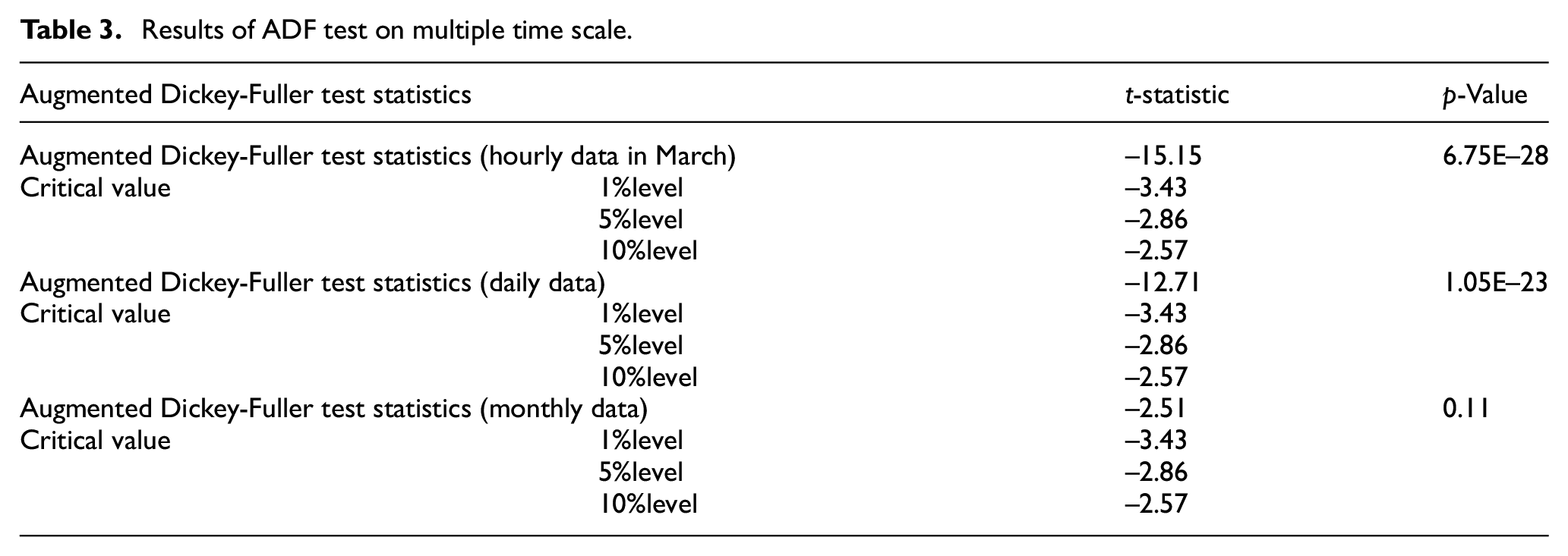
until the time series is stable. And the other two stationary time series samples do not need differential processing.

Methodology

Since wind speed time series is seasonal, we use STL decomposition method to eliminate the seasonal factors. Moreover, wind speed time series has nonlinearity and randomness, which make it difficult to accurately predict future wind speed as well, so we propose to adopt the hybrid method of ARIMA and LSTM to increase the forecast precision.

The framework of the proposed model

Figure 4 shows the flow chart of our proposed model, which has the following four steps.

Firstly, as mentioned above, the raw wind speed time series are preprocessed, where the multi-scale samples involving hourly, daily and monthly data are obtained by downsampling processing.

Then, STL decomposition method is used to eliminate the seasonal components in the subsamples. In the process of STL decomposition, only the training set is used, and there is no risk of test set information leakage.

After seasonal adjustment for the 3 time scale samples, ARIMA is applied to predict the time series to obtain prediction values and residual series.

For the residual series, another part prediction results are obtained by using LSTM neural network. The final prediction results are obtained by adding the two part results computed by ARIMA model and LSTM neural network respectively.

Figure 4.

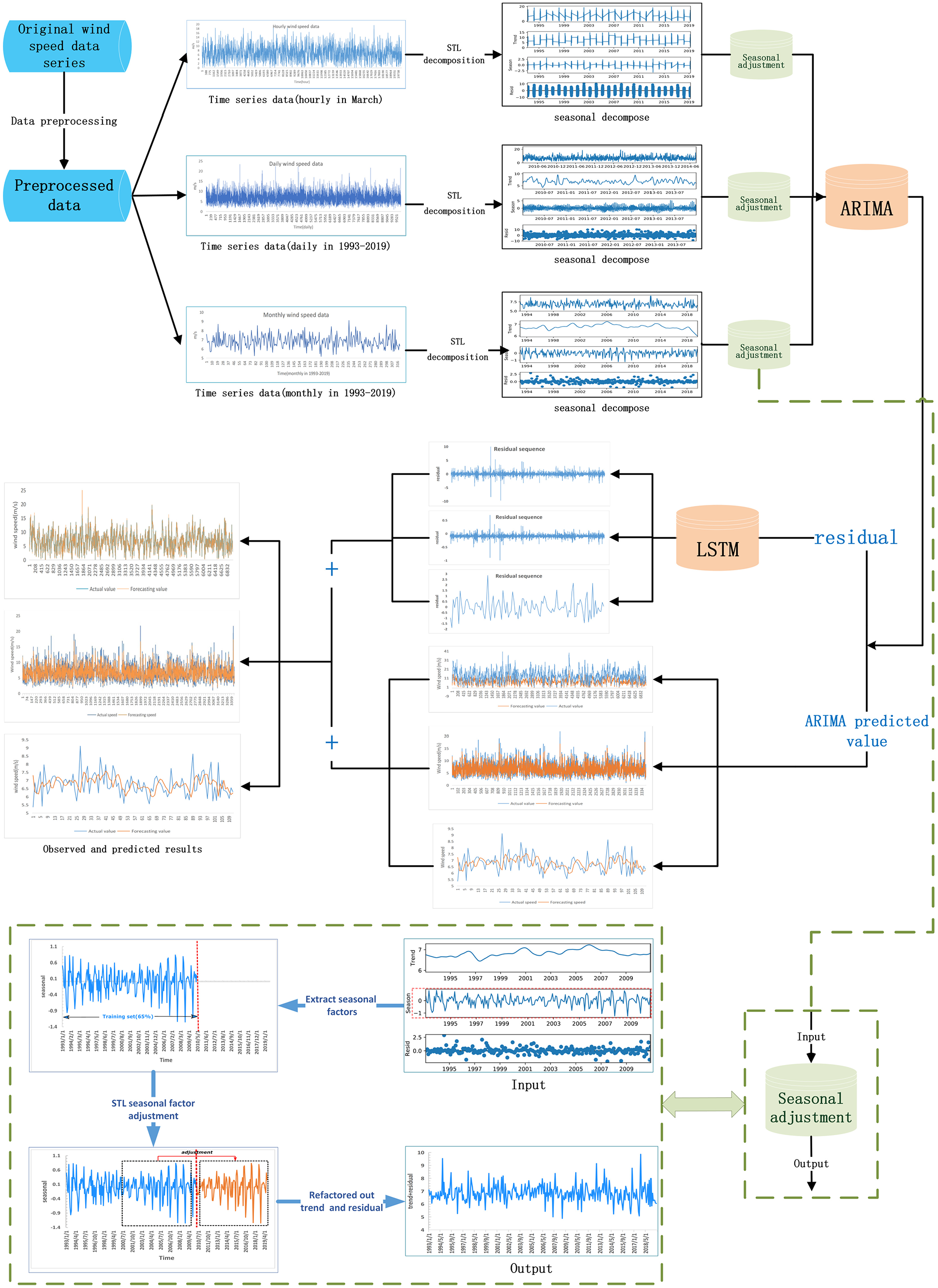
Framework of hybrid models.

STL

STL is a classical time series decomposition technique. Its significant advantage is that it can decompose the time series with outliers into robust components (Theodosiou, 2011; Yang et al., 2021). Based on STL method, the sequence can be decomposed into the following three components

X_{t} = S_{t} + T_{t} + R_{t},

(3)

where $X_{t}$ , $S_{t}$ , $T_{t}$ , and $R_{t}$ denote the original time series data, seasonal components, trend components, and residual components respectively (Chaloupka, 2001; He et al., 2021). The STL procedure is carried out based on numerical methods, and the STL algorithm consists of two recursive processes: an inner loop and an outer loop.

The inner loop iteration is to update the corresponding seasonal and trend components. Each time the inner loop is completed, the robustness weights will be calculated in the outer loop, and then the weights will be used to reduce the impact of outliers on the update, which is the impact on the seasonal and trend components in the next inner loop. Figure 5 shows the steps of the inner loop (Yang et al., 2021):

Figure 5.

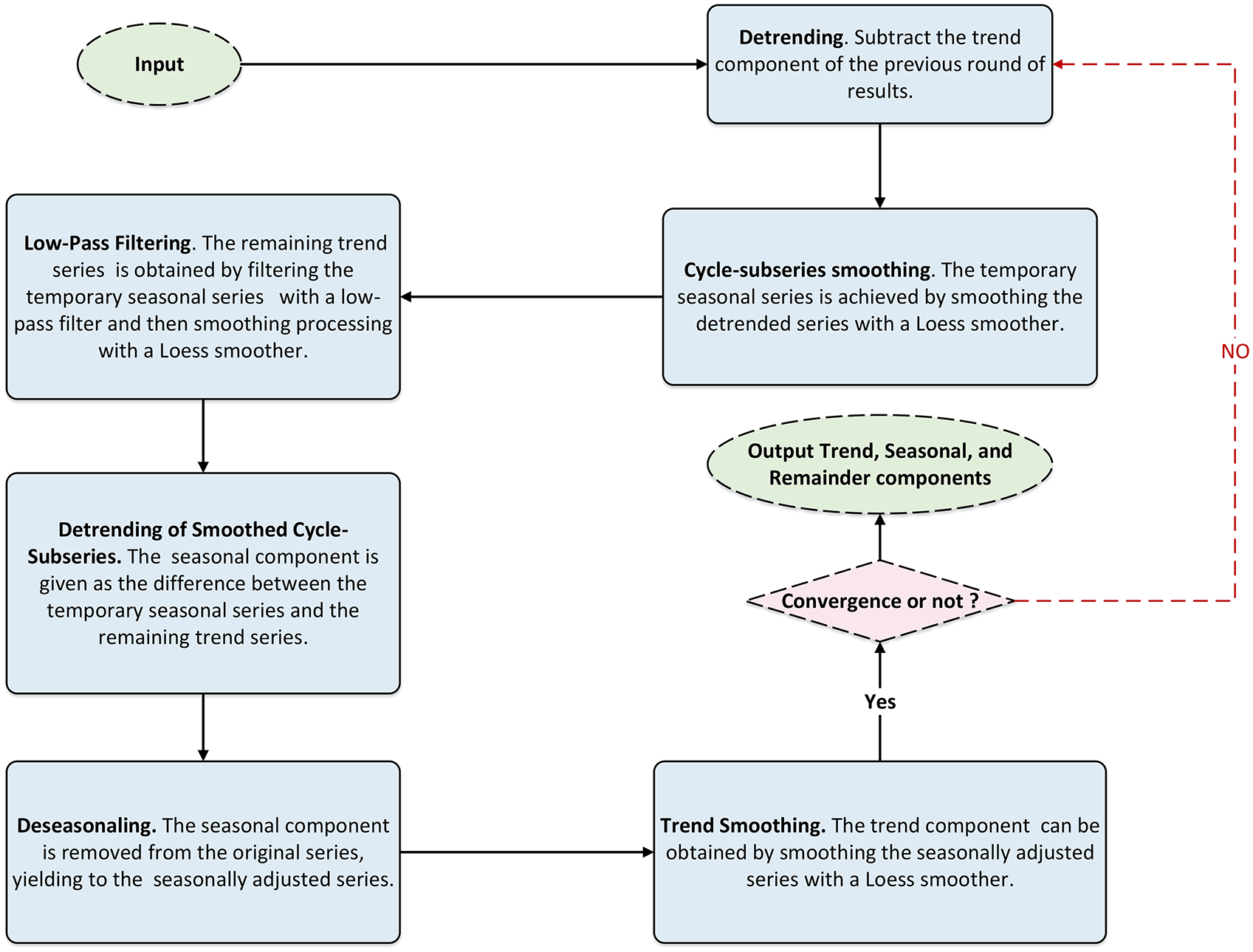
The inner loop of STL decomposition.

In the outer loop, the trend and seasonal components obtained in the inner loop are employed to calculate the remaining component through the formula $R_{t}^{(k + 1)} = X_{t} - S_{t}^{(k + 1)} - T_{t}^{(k + 1)}$ . All values satisfying $| R_{t} | > A$ where $A$ is a fixed large number and its weights are computed. These weights can be used in the next iteration of the inner loop to reduce the influence of outliers.

The above process is the implementation procedure of decomposing the raw sequence into seasonal components, trend components and remainder components.

ARIMA

ARIMA is a predicting technique of time sequence. ARIMA has the characteristics of differential transformation, autoregressive and moving average (Zhang, 2003). In addition, ARIMA is a method established by regressing the lagging value of dependent variables and the present value and lagging value of random error term (Box and Jenkins, 1970). Therefore, ARIMA model is usually used for wind speed prediction because it only needs endogenous variables and does not need other exogenous variables, as well as is easy to implement.

The basic idea of ARIMA is that the data sequence formed by the prediction object over time is regarded as a random sequence. Its formula is expressed as follows

\begin{matrix} X_{t} = φ_{0} X_{t - d} + φ_{1} X_{t - d - 1} + \dots + φ_{p} X_{t - d - p} + ε_{t} \\ - θ_{1} ε_{t - 1} - θ_{2} ε_{t - 2} - \dots - - θ_{q} ε_{t - q} . \end{matrix}

(4)

The formula can also be expressed as follows

φ_{B} (1 - B)^{d} X_{t} = θ (B) ε_{t}, t \in Z .

(5)

Eq.4 contains two important special cases of ARIMA model. When using ARIMA model, the most important thing is to determine the parameters of the model, that is, $(p, d, q)$ . The parameter determination process of ARIMA in this paper is given in Section “Experiments.”

LSTM

As a special RNN, LSTM proposed by Hochreiter and Schmidhuber (1997) can avoid vanishing gradient and exploding gradient problems that usually occur in initial RNN (You and Nikolaou, 1993). On this basis, Gers et al. (2000) added the forget gate to release the internal resources in the LSTM cell, so the current LSTM neuron includes three gates: inputting, forgetting and outputting gates, as shown in Figure 6. This structure can not only effectively mine and utilize the hidden information in dynamic time series, but also automatically store and delete time state information. The neuron of LSTM is like a special built-in memory block, which can extract the complex feature relationships between long-time series and short-time series (Gers et al., 2000; Hochreiter and Schmidhuber, 1997). Therefore, LSTM neural network has unique advantages in the processing of time series prediction (Chen et al., 2018).

Figure 6.

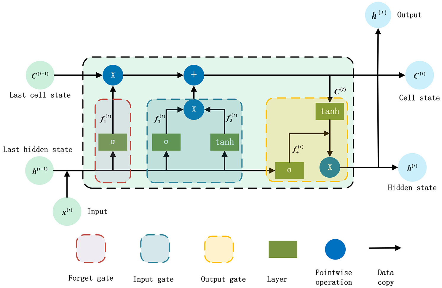
Internal structure of LSTM neurons.

Forget gate: The task of the forget gate is to accept a longterm memory $C^{(t - 1)}$ , and control which part of the $C^{(t - 1)}$ to keep or forget. The mathematical principle is multiply the longterm memory input $C^{(t - 1)}$ at time $t - 1$ by a forgetting factor $f_{1}^{(t)}$ . The forgetting factor $f_{1}^{(t)}$ is calculated by shortterm memory $h_{t - 1}$ and event input information $x_{t}$ as follows

f_{1}^{(t)} = σ (W_{f 1} \times [h^{(t - 1)}, x^{(t)}] + b_{1}),

(6)

where $σ$ , $W_{fi}$ and $b_{i}$ are the sigmoid function, the weight matrices and the bias, respectively.

Input gate: It determines the input $x^{(t)}$ at the current time $t$ and how many are saved to cell state. The first step is to decide what values need to be updated through the sigmoid layer, and the second step is to create a new candidate value vector and generate candidate memory through the tanh layer. The update value $f_{2}^{(t)}$ and the candidate state $f_{3}^{(t)}$ are given by the following algorithms

f_{2}^{(t)} = σ (W_{f 2} \times [h^{(t - 1)}, x^{(t)}] + b_{2}),

(7)

f_{3}^{(t)} = \tanh (W_{f 3} \times [h^{(t - 1)}, x^{(t)}] + b_{3}) .

(8)

Then, the new neuron state value $C^{(t)}$ at time $t$ can be obtained by integrating the previous information according to the expression

C^{(t)} = C^{(t - 1)} \times f_{1}^{(t)} + f_{2}^{(t)} \times f_{3}^{(t)},

(9)

Output gate: It calculates the output information according to the state of the unit. The output factor $f_{4}^{(t)}$ is obtained by a sigmoid function. Then $f_{4}^{(t)}$ is multiplied by $\tanh (C^{(t)})$ to obtain the final output $h_{4}^{(t)}$ according to the following formula

f_{4}^{(t)} = σ (W_{f 4} \times [h^{(t - 1)}, x^{(t)}] + b_{4}),

(10)

h_{4}^{(t)} = f_{4}^{(t)} \times \tanh (C^{(t)}) .

(11)

Experiments

This section briefly introduces the methods of seasonal adjustment and the configuration of each test method. In this experiment, the feasibility of the model is verified by three examples on different time scales. Training set consists of the first 65% of the data, and the remaining 35% of the data constitute the test set.

Seasonal adjustment

Monthly average wind speed distribution is shown in Figure 7, from which it can be found that the wind speed sequence has obvious seasonality. In order to make the wind speed prediction more accurate, the STL decomposition method is used to eliminate the seasonal characteristics. In the process of time series decomposition, the problem of information leakage must be paid attention to. Figure 8 illustrates our STL seasonal adjustment preprocessing data process, which can avoid information leakage. The specific implementation process is as follows. A part data from the target wind speed series $X_{t}$ are selected to form the training set $X_{train}$ , and then remaining data constitute the test set $X_{test}$

X_{t} = (X_{train}, X_{test}) .

(12)

Figure 7.

Monthly average wind speed from 1993 to 2019.

Figure 8.

STL seasonal adjustment preprocessing data process.

STL adjustment is implemented on the training set $X_{train}$ , which is decomposed into the season term $S_{train}$ , the trend term $T_{train}$ , and the residual term $R_{train}$ as follows

X_{train} = S_{train} + T_{train} + R_{train} .

(13)

An example of wind speed time series for STL framework and decomposition is shown in Figure 9.

Figure 9.

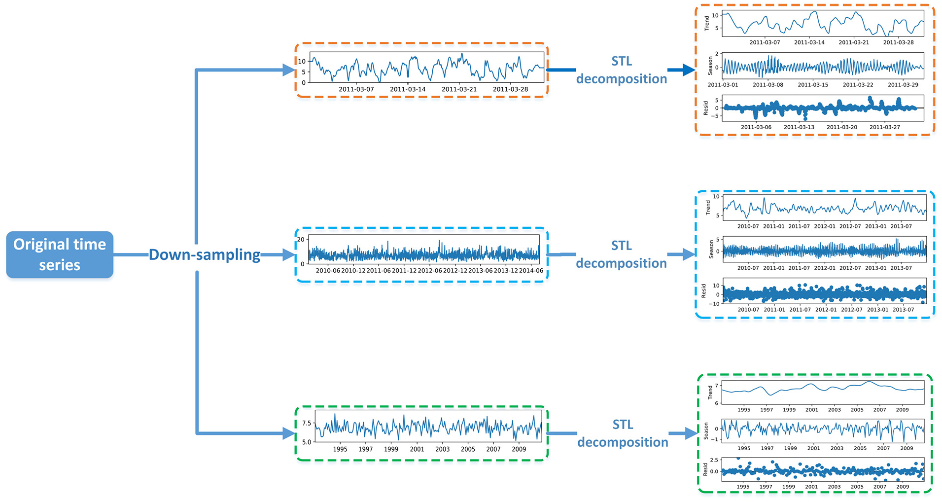
STL decomposition of wind speed series in training set.

Because the seasonal component $S_{train}$ is periodic, it can be used to predict the seasonal term of wind speed time sequences. $S_{test}$ denotes the prediction result of seasonal term in the test set, and then $S_{predict}$ as a complete data set after seasonal adjustment can be written as

S_{predict} = (S_{train}, S_{test}) .

(14)

The output item of seasonal adjustment $X_{out}$ can be obtained by subtracting $S_{predict}$ from $X_{t}$ as follows

X_{out} = X_{t} - S_{predict} .

(15)

After that, just substitute $X_{out}$ into the prediction model for prediction. This processing method can not only remove the seasonal factors in the sequence, but also avoid leaking the information of the test set to the future model (ARIMA-LSTM) training.

Experimental parameter settings

Based on the proposed STL-ARIMA-LSTM hybrid method, this paper predicts three sub-sample data sets with different time scales. The performance of STL-ARIMA-LSTM hybrid model is comprehensively investigated by comparing with ARIMA model, LSTM model, STL-ARIMA model, STL-LSTM model, and ARIMA-LSTM hybrid model in each sample data set.

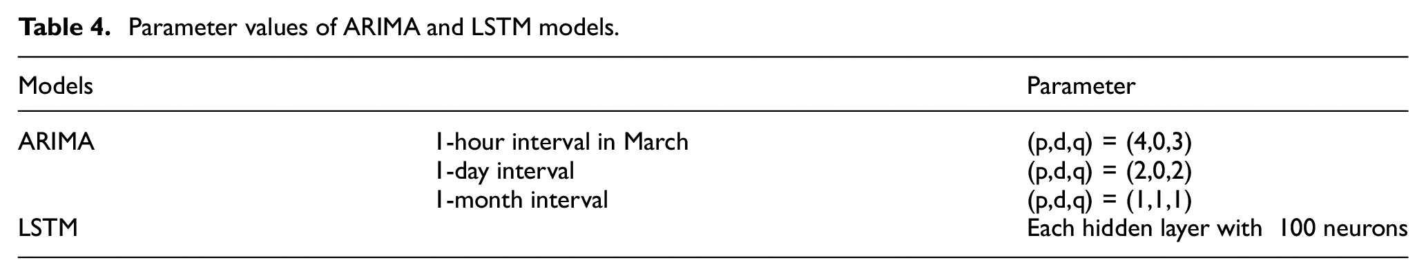
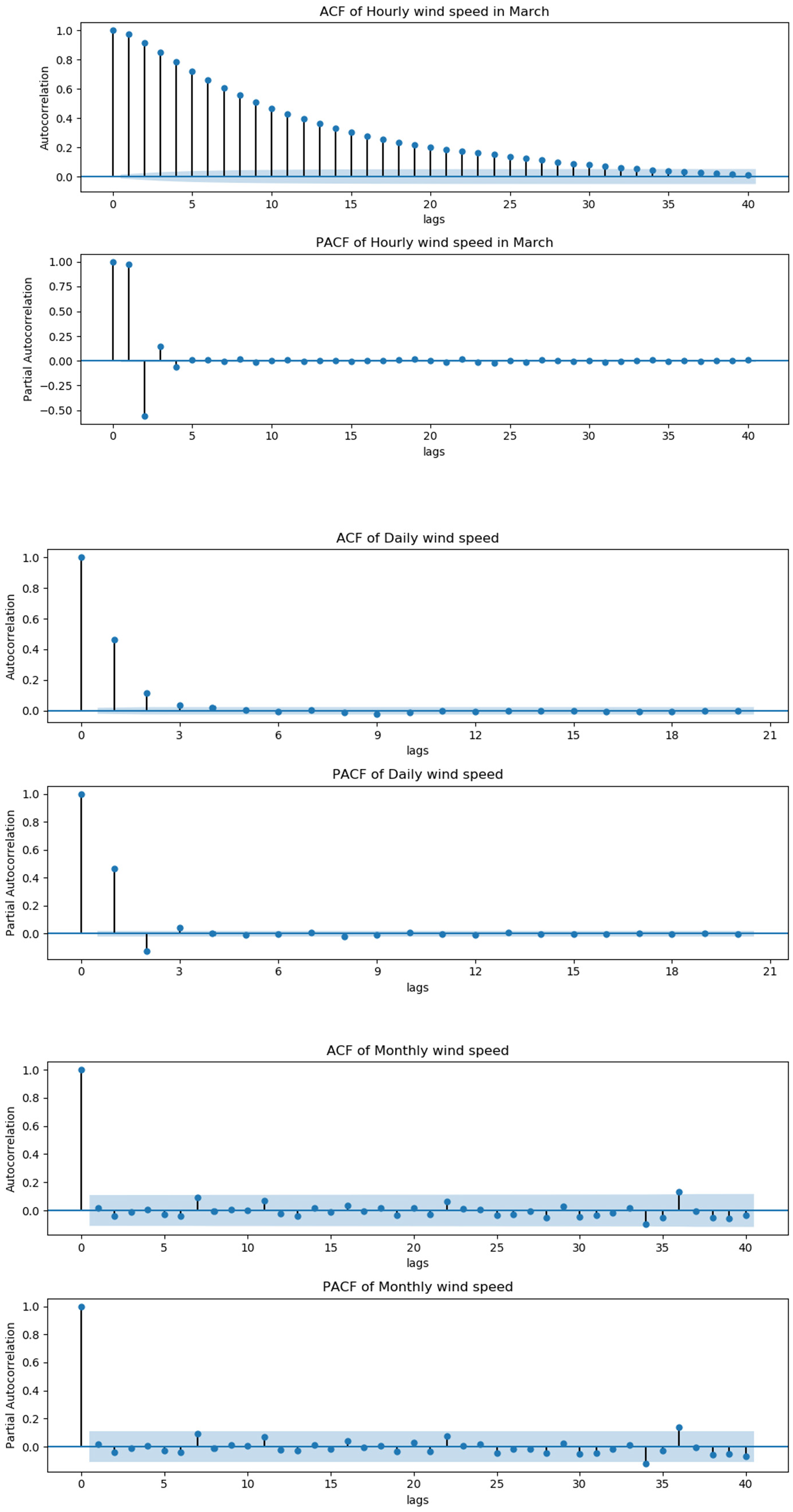
Some special parameters in the prediction model need to be determined in advance. In ARIMA model, the initial range of $(p, d, q)$ is set according to the ACF diagram and the PACF diagram which are shown in Figure 10. AIC and BIC constitute an evaluator for comparing models. The lower AIC value and BIC value, the better ARIMA model. The minimum order combination of AIC and BIC can be automatically realized by calling auto.arima function in the Pmdarima package of Python program, and then the parameters $(p, d, q)$ are given as shown in Table 4. In LSTM model, each hidden layer with 100 neurons is set by several repeated tests and adjustments.

Figure 10.

Autocorrelation and partial correlation graphs of sample time series.

Table 4.

Parameter values of ARIMA and LSTM models.

Models		Parameter
ARIMA	1-hour interval in March	(p,d,q) = (4,0,3)
	1-day interval	(p,d,q) = (2,0,2)
	1-month interval	(p,d,q) = (1,1,1)
LSTM		Each hidden layer with 100 neurons

Results

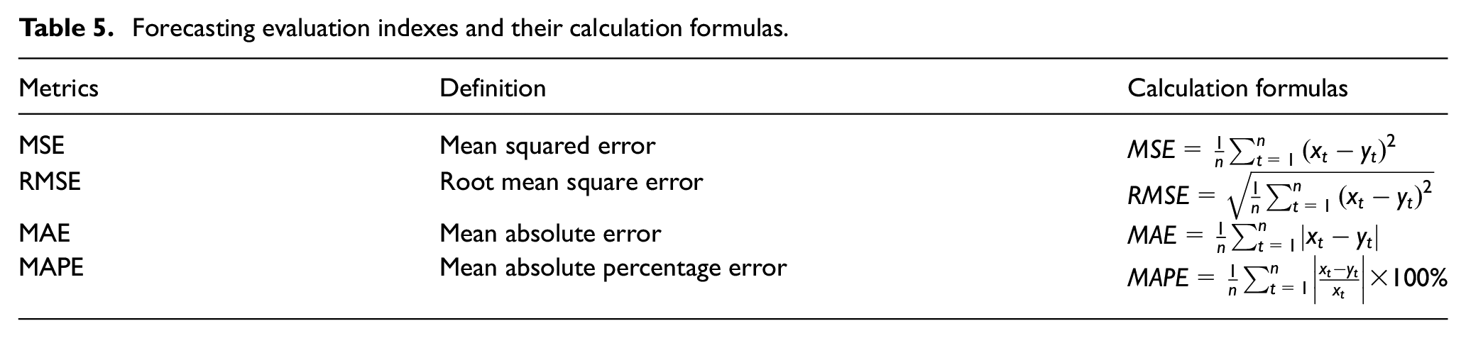
In this article, we will use four model performance indexes, namely MSE, RMSE (Foley et al., 2012; Kavasseri and Seetharaman, 2009), MAE (Foley et al., 2012), and MAPE (He et al., 2021). These indexes can be used to evaluate the performance of the prediction model. Table 5 shows the formulas of different evaluation indexes, where $x_{t}$ means actual wind speeds, $y_{t}$ means predicted wind speeds, and $n$ means the number of time steps. The four indicators are to assess the difference between real values and prediction results. The lower their value, the higher the accuracy and the better the prediction effect.

Table 5.

Forecasting evaluation indexes and their calculation formulas.

Metrics	Definition	Calculation formulas
MSE	Mean squared error	$MSE = \frac{1}{n} \sum_{t = 1}^{n} (x_{t} - y_{t})^{2}$
RMSE	Root mean square error	$RMSE = \sqrt{\frac{1}{n} \sum_{t = 1}^{n} {(x_{t} - y_{t})}^{2}}$
MAE	Mean absolute error	$MAE = \frac{1}{n} \sum_{t = 1}^{n} \| x_{t} - y_{t} \|$
MAPE	Mean absolute percentage error	$M A P E = \frac{1}{n} \sum_{t = 1}^{n} \| \frac{x_{t} - y_{t}}{x_{t}} \| \times 100 %$

Case 1: Very shortterm wind speed prediction

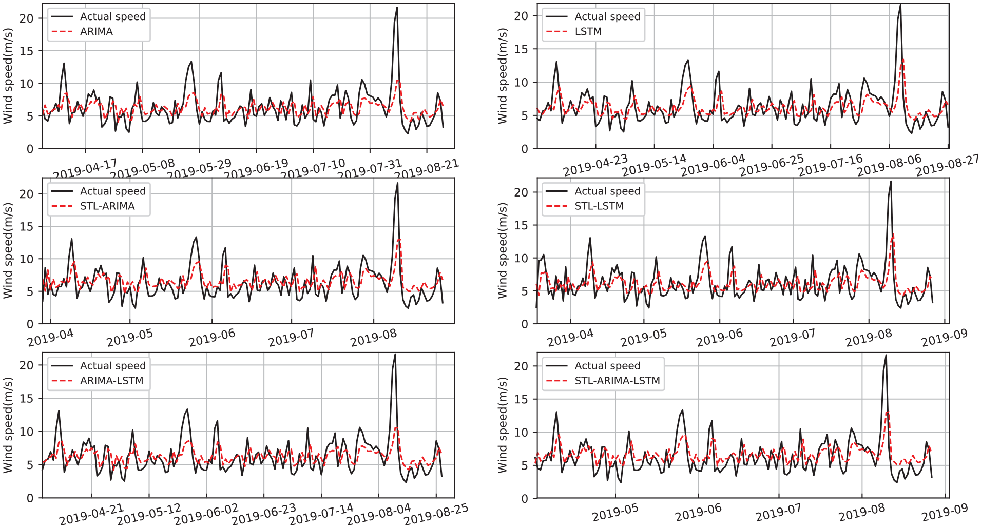
In case 1, we selected the hourly wind speed series in March from 1993 to 2019 to constitute the data set. This wind speed series belongs to a very shortterm time scale type. Figure 11 shows the prediction results of ARIMA model, LSTM model, STL-ARIMA model, STL-LSTM model, ARIMA-LSTM model, and STL-ARIMA-LSTM hybrid model. It seems clear that the prediction results of all models are in good agreement with the actual wind speed time sequences. Compared with the other five models, the proposed model well deals with the lag of the predicted value, and fits the actual wind speed best. In particular, STL-ARIMA-LSTM hybrid model achieves the best prediction result, which can be further verified by error evaluation indexes. Figure 12 illustrates the values of error evaluation indexes including MSE, RMSE, MAE and MAPE for the six prediction models. Accordingly, these values are summarized in Table 6 which includes all evaluation index of very shortterm wind time series for eight different prediction models. And the values given in bold indicate the minimum error value. We also added the prediction results of RF and SVM models in this table. In this way, the prediction effect of this model can be more prominent.

Figure 11.

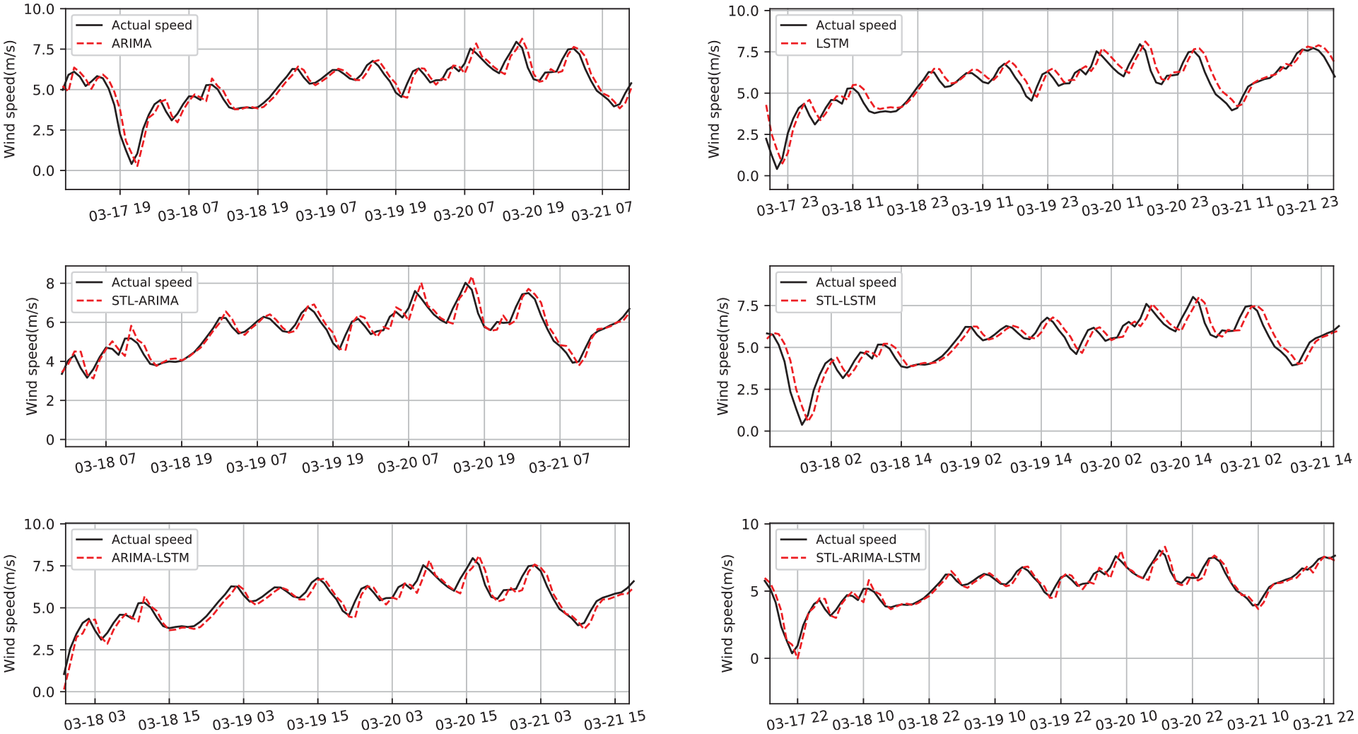
The wind speed forecasting results of very shortterm wind speed.

Figure 12.

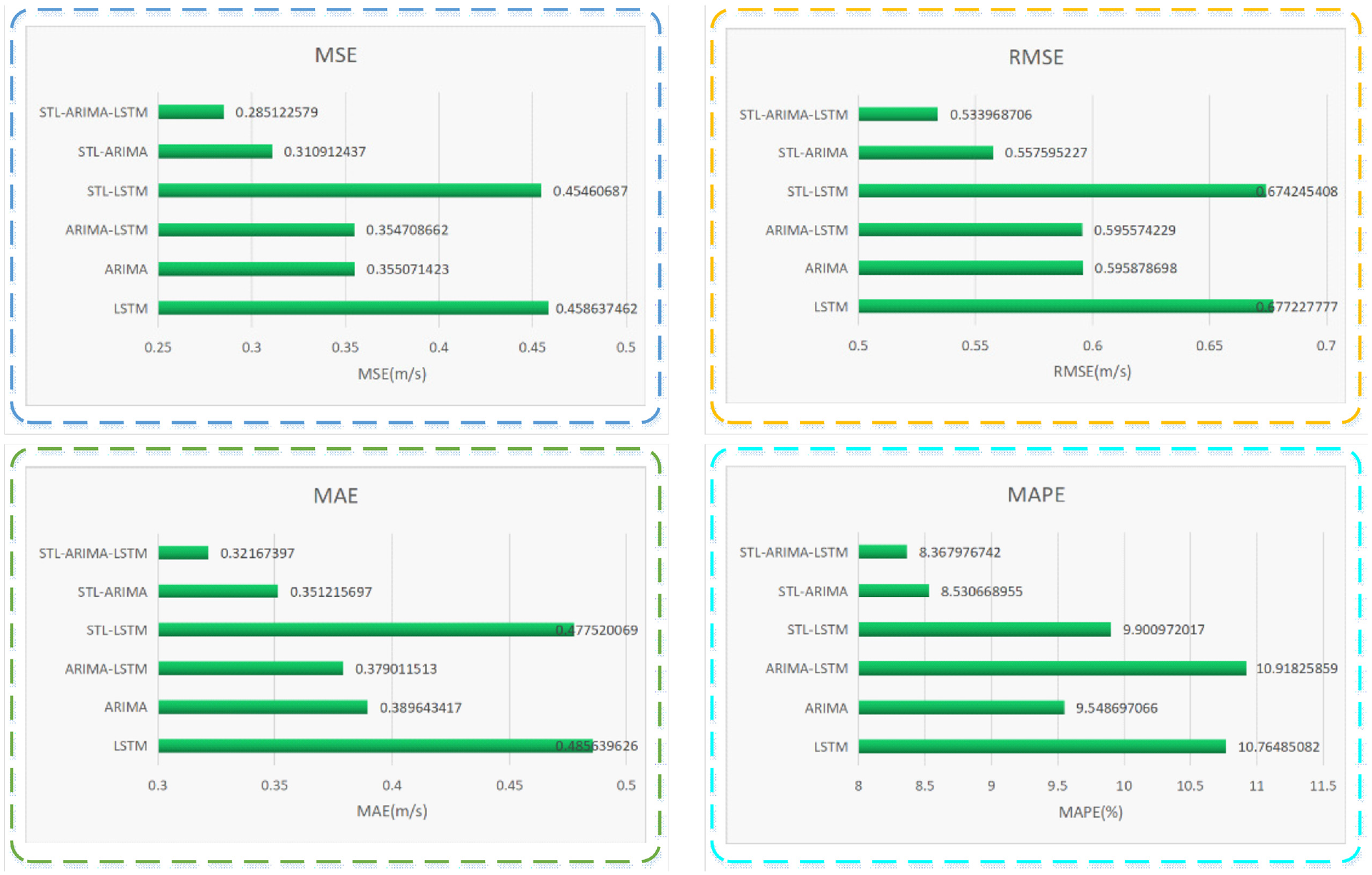
Histogram of forecast indexes of very shortterm wind speed.

Table 6.

Very shortterm forecasting performance indices and their definition.

	RF	SVM	ARIMA	STL-ARIMA	LSTM	STL-LSTM	ARIMA-LSTM	STL-ARIMA-LSTM
MSE (m/s)	0.32152	0.45067	0.35507	0.31091	0.45864	0.45461	0.35471	0.28512
RMSE (m/s)	0.56702	0.67132	0.59588	0.55760	0.67723	0.67425	0.59557	0.53397
MAE (m/s)	0.35734	0.35956	0.38964	0.35122	0.48564	0.47752	0.37901	0.32167
MAPE (%)	8.87826	9.58589	9.54870	8.53067	10.76485	9.90097	10.91826	8.36798

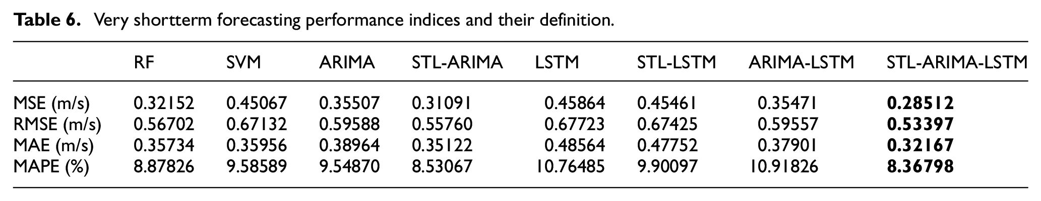
From the results of evaluation indicators, the prediction results of the proposed model are better than those of RF and SVM. Therefore, in the Figures 11 and 12, we only consider the six comparison models related to this STL-ARIMA-LSTM model for comparison. In this way, the comparative analysis can be carried out layer by layer, which reflects the advantages of this model. For this very shortterm wind speed prediction, whether from Figures 11 and 12 or Table 6, we can see that the error of STL-ARIMA-LSTM hybrid model is the smallest compared with the other forecast models. In fact, MSE, RMSE, MAE, and MAPE of STL-ARIMA-LSTM model are 0.2851, 0.5340, 0.3217, and 8.3679%, respectively. The error of LSTM is the largest, where its MSE, RMSE, MAE, and MAPE are 0.4586, 0.6772, 0.4856, and 10.7649%, respectively. This also indicates that data preprocessing and seasonal component removal can greatly improve the accuracy of model prediction.

Case 2: Shortterm wind speed prediction

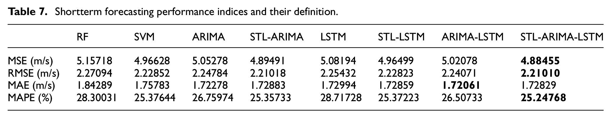
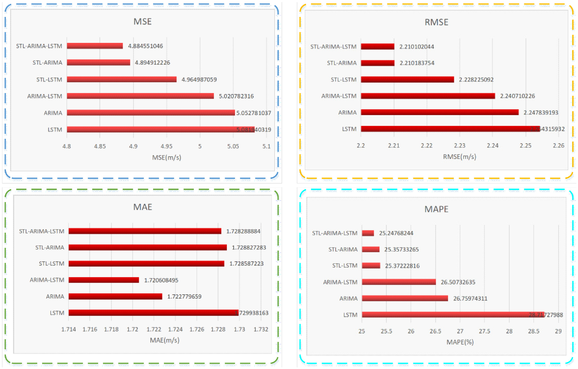
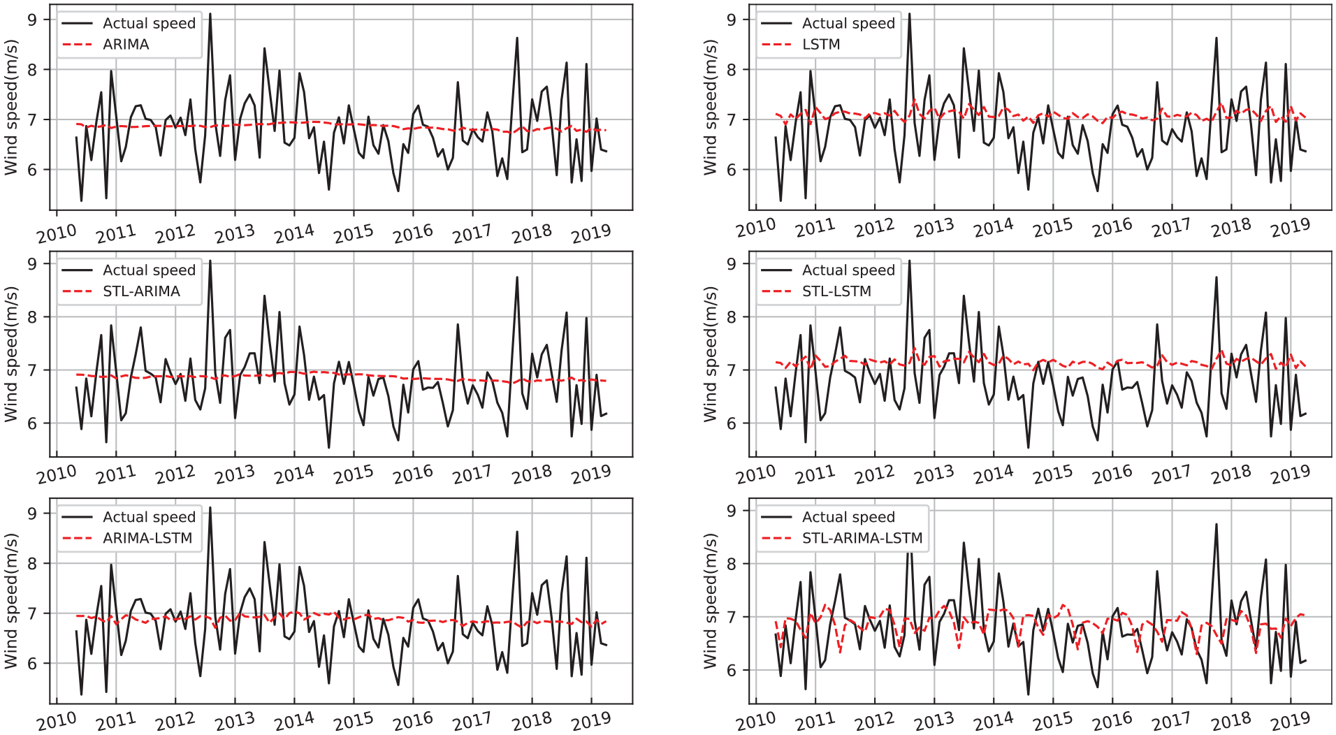
Case 2 investigates the daily average wind speed series from January 1, 1993 to August 31, 2019, which belongs to a shortterm time scale type. The last 35% of the data which form test set involve the wind speed time series from April 30, 2010 to August 31, 2019. Figure 13 shows the prediction results of ARIMA model, LSTM model, STL-ARIMA model, STL-LSTM model, ARIMA-LSTM model, and STL-ARIMA-LSTM model in comparison with the test data. Compared with 1-hour interval wind speed, 1-day interval wind speed fluctuates more, with more extreme values and the amount of data is also reduced, which greatly increases the difficulty of model prediction. Nevertheless, it can be observed that the change trends of the prediction results of six models are generally correct, although the wind speed prediction results of case 2 are not as good as those of case 1. Table 7 shows the results of shortterm wind speed prediction evaluation indicators for the eight models. Combined with the values of error evaluation indexes involving MSE, RMSE, MAE, and MAPE, as shown in Figure 14 and Table 7, the prediction results are all within a reasonable and acceptable range.

Figure 13.

The wind speed forecasting results of shortterm wind speed.

Table 7.

Shortterm forecasting performance indices and their definition.

	RF	SVM	ARIMA	STL-ARIMA	LSTM	STL-LSTM	ARIMA-LSTM	STL-ARIMA-LSTM
MSE (m/s)	5.15718	4.96628	5.05278	4.89491	5.08194	4.96499	5.02078	4.88455
RMSE (m/s)	2.27094	2.22852	2.24784	2.21018	2.25432	2.22823	2.24071	2.21010
MAE (m/s)	1.84289	1.75783	1.72278	1.72883	1.72994	1.72859	1.72061	1.72829
MAPE (%)	28.30031	25.37644	26.75974	25.35733	28.71728	25.37223	26.50733	25.24768

Figure 14.

Histogram of forecast indexes of shortterm wind speed.

Among all the models, STL-ARIMA-LSTM model has the smallest error in terms of MSE=4.8846, RMSE=2.2108, and MAPE=25.25%, ignoring its MAE index with no obvious advantage. Furthermore, combined with the fitting effect between the predicted data and test data, the wind speed time series predicted by STL-ARIMA-LSTM model is closest to the actual wind speed.

Case 3: Longterm wind speed prediction

Case 3 selects the monthly average wind speed series from January 1993 to August 2019 to form the data set with longterm time scale type. The first 65% of the data which form the train set consist of the wind speed time sequences from January 1993 to March 2010. Figure 15 shows the prediction results of ARIMA model, LSTM model, STL-ARIMA model, STL-LSTM model, ARIMA-LSTM model, and STL-ARIMA-LSTM model for this longterm time sequences. Among these 3 time scales of wind speed time sequences, the uncertainty, intermittence and volatility of long-time scale wind speed series are the most sufficient and strongest, which poses a great challenge to the accuracy of prediction. Here, except that the new model STL-ARIMA-LSTM proposed better captures the periodic trend of longterm wind speed time sequences, the prediction models do not well capture the intermittence, shock and extreme value. Still, we observe that the prediction result curve of LSTM can better reflect the periodicity of time series than that of ARIMA, which indicates that LSTM has more advantage in predicting nonlinear time series, while ARIMA predicts better in linear time series.

Figure 15.

The wind speed forecasting results of longterm wind speed.

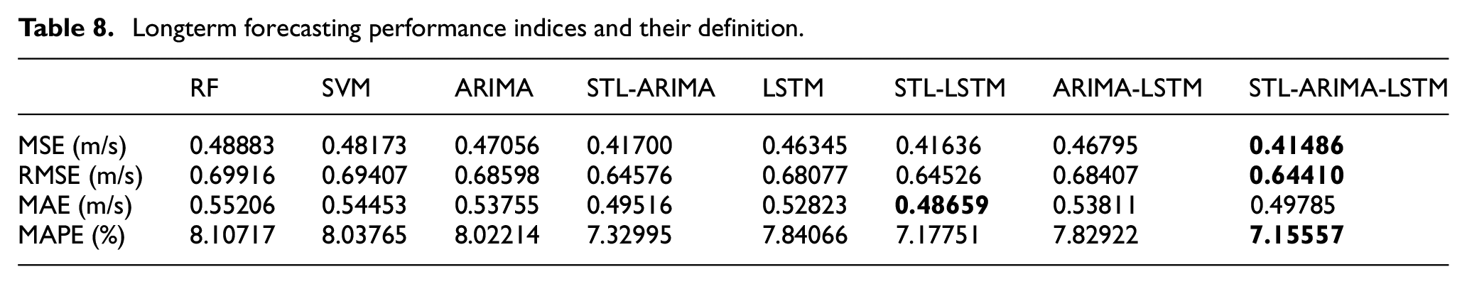
Table 8 shows the results of longterm wind speed prediction evaluation indexes for eight models. As can be seen from Figures 15 and 16 and Table 8, LSTM based on STL, namely STL-LSTM, has higher accuracy than LSTM without STL. Specifically, by comprehensively considering four performance evaluation indicators, STL-ARIMA-LSTM hybrid model has the best prediction accuracy, where the performance of STL-ARIMA-LSTM with MSE = 0.4149, RMSE = 0.6441, and MAPE = 7.1556% is obviously better than the other seven models. MAE value of STL-ARIMA-LSTM is slightly greater than those of STL-ARIMA and STL-LSTM, but the difference between the three models is not as obvious as that between the other three models without SLT. In conclusion, based on the analysis of performance evaluation indexes and prediction results, STL-ARIMA-LSTM model has the best prediction results for longterm wind speed time sequences, which has been better verified in very shortterm and shortterm wind speed predicting as well.

Table 8.

Longterm forecasting performance indices and their definition.

	RF	SVM	ARIMA	STL-ARIMA	LSTM	STL-LSTM	ARIMA-LSTM	STL-ARIMA-LSTM
MSE (m/s)	0.48883	0.48173	0.47056	0.41700	0.46345	0.41636	0.46795	0.41486
RMSE (m/s)	0.69916	0.69407	0.68598	0.64576	0.68077	0.64526	0.68407	0.64410
MAE (m/s)	0.55206	0.54453	0.53755	0.49516	0.52823	0.48659	0.53811	0.49785
MAPE (%)	8.10717	8.03765	8.02214	7.32995	7.84066	7.17751	7.82922	7.15557

Figure 16.

Histogram of forecast indexes of longterm wind speed.

Conclusions

This article presents a new STL-ARIMA-LSTM model for wind speed prediction on 3 time scales: very shortterm, shortterm, and longterm. The main work and conclusions are as follows.

In order to accurately and fully mine the data information, the wind speed time sequences is preprocessed and statistically analyzed. We handle the missing values by interpolation, perform the T-test to test the data differences between 2 adjacent years and 2 months corresponding to adjacent years, give descriptive statistics of data on 3 time scales to get an intuitive understanding on the distribution pattern and volatility of wind speed time sequences, and test the stationarity of dimensionless normalization data on 3 time scales by using ADF test method.

Since the wind speed time series has obvious seasonality, STL decomposition method is applied to eliminate seasonal component in wind speed time sequences, so it can achieve accurate prediction of wind speed. Especially, in the experiment, in order to avoid the problem of information leakage, we implement two strategies: (a) distinguishing the training set from the test set in the process of standardization; (b) only performing STL decomposition on the wind speed data of train set. For seasonally adjusted wind speed time series, ARIMA-LSTM hybrid model is proposed to predict the time series, which can make full use of the advantages of ARIMA in processing linear time series and LSTM in processing nonlinear time series. We refer to the proposed model as STL-ARIMA-LSTM hybrid model here.

Finally, STL-ARIMA-LSTM model is applied to compute wind speed time sequences with very shortterm, shortterm, and longterm respectively. Meanwhile, its performance has been validated by comparing with RF, SVM, ARIMA, LSTM, ARIMA-LSTM, STL-ARIMA, and STL-LSTM models. The results reveal that the STL-ARIMA-LSTM hybrid model has the highest accuracy and the highest resolution for the trend and periodicity of wind speed series on 3 time scales among eight prediction models. In the 3 time-scale wind speed time sequences prediction, the proposed model has the best prediction result on the 1-hour interval wind speed time sequences, and can solve the problem of lag in forecasting. For 1-day interval and 1-month interval wind speed time sequences, as the time interval of data increases, the uncertainty, intermittence, volatility increase sharply and the amount of data decreases. This leads to the prediction models can not well capture the intermittence, extreme value and volatility with high frequency and wide amplitude, whereas STL-ARIMA-LSTM better captures the periodic trend of different time intervals wind speed than the other seven models.

In the experimental analysis of three cases, we found that due to the different time scales of wind speed data, the fluctuation and amplitude of data are very different, which also affects the accuracy of model prediction. Therefore, when predicting the wind speed, we can first try to calculate the wind speed series on a longterm time scale to achieve an overall grasp for the problem, and then handle the strong intermittence, volatility with high frequency and wide amplitude, and outliers in the wind speed by gradually adjusting the time scale.

Footnotes

Appendix

Declaration of conflicting interests

The author(s) declared no potential conflicts of interest with respect to the research, authorship, and/or publication of this article.

Funding

The author(s) disclosed receipt of the following financial support for the research, authorship, and/or publication of this article: This work was supported by the Science and Technology Project of State Grid Shanghai Municipal Electric Power Company (No. 52090R19000C).

ORCID iD

Li Xu

References

Aasim Singh

S N

Mohapatra

(2019) Repeated wavelet transform based ARIMA model for very short-term wind speed forecasting. Renewable Energy 136: 758–768.

Afshar

Ghiasvand

Bigdeli

(2018) Optimal bidding strategy of wind power producers in pay-asbid power markets. Renewable Energy 127: 575–586.

Benth

JŠ

Benth

(2010) Analysis and modelling of wind speed in New York. Journal of Applied Statistics 37(6): 893–909.

Boutoubat

Mokrani

Machmoum

(2013) Control of a wind energy conversion system equipped by a DFIG for active power generation and power quality improvement. Renewable Energy 50: 378–386.

Box

Jenkins

(1970) Time series analysis forecasting and control. Operational Research Quarterly 22: 199–201.

Cadenas

Rivera

(2010) Wind speed forecasting in three different regions of Mexico, using a hybrid ARIMA–ANN model. Renewable Energy 35(12): 2732–2738.

Chaloupka

(2001) Historical trends, seasonality and spatial synchrony in green sea turtle egg production. Biological Conservation 101(3): 263–279.

Chen

Zeng

Zhou

, et al. (2018) Wind speed forecasting using nonlinear-learning ensemble of deep learning time series prediction and extremal optimization. Energy Conversion and Management 165: 681–695.

Chen

Zhang

, et al. (2019) Multifactor spatio-temporal correlation model based on a combination of convolutional neural network and long short-term memory neural network for wind speed forecasting. Energy Conversion and Management 185: 783–799.

10.

Cleveland

(1990) Stl: A seasonal-trend decomposition procedure based on loess. Journal of Official Statistics 6: 3–73.

11.

Erdem

Shi

(2011) ARMA based approaches for forecasting the tuple of wind speed and direction. Applied Energy 88(4): 1405–1414.

12.

Foley

Leahy

Marvuglia

, et al. (2012) Current methods and advances in forecasting of wind power generation. Renewable Energy 37(1): 1–8.

13.

Gers

Schmidhuber

Cummins

(2000) Learning to forget: Continual prediction with LSTM. Neural Computation 12(10): 2451–2471.

14.

Gao

Jin

, et al. (2021) A seasonal-trend decomposition-based dendritic neuron model for financial time series prediction. Applied Soft Computing 108: 107488.

15.

Hochreiter

Schmidhuber

(1997) Long short-term memory. Neural Computation 9(8): 1735–1780.

16.

Hur

(2021) Short-term wind speed prediction using extended Kalman filter and machine learning. Energy Reports 7: 1046–1054.

17.

Jaseena

Kovoor

(2021) Decomposition-based hybrid wind speed forecasting model using deep bidirectional LSTM networks. Energy Conversion and Management 234: 113944.

18.

Kavasseri

Seetharaman

(2009) Day-ahead wind speed forecasting using f-ARIMA models. Renewable Energy 34(5): 1388–1393.

19.

Khodayar

Wang

Manthouri

(2019) Interval deep generative neural network for wind speed forecasting. IEEE Transactions on Smart Grid 10(4): 3974–3989.

20.

Krämer

(1998) Fractional integration and the augmented Dickey–Fuller test. Economics Letters 61(3): 269–272.

21.

Lin

Kruger

Zhang

, et al. (2015) Seasonal analysis and prediction of wind energy using random forests and ARX model structures. IEEE Transactions on Control Systems Technology 23(5): 1994–2002.

22.

Liu

(2018a) Smart multi-step deep learning model for wind speed forecasting based on variational mode decomposition, singular spectrum analysis, LSTM network and ELM. Energy Conversion and Management 159: 54–64.

23.

Liu

(2018b) Wind speed forecasting method based on deep learning strategy using empirical wavelet transform, long short term memory neural network and Elman neural network. Energy Conversion and Management 156: 498–514.

24.

Liu

(2020) Multi-step wind speed forecasting model based on wavelet matching analysis and hybrid optimization framework. Sustainable Energy Technologies and Assessments 40: 100745.

25.

Memarzadeh

Keynia

(2020) A new short-term wind speed forecasting method based on fine-tuned LSTM neural network and optimal input sets. Energy Conversion and Management 213: 112824.

26.

Mohandes

Halawani

Rehman

, et al. (2004) Support vector machines for wind speed prediction. Renewable Energy 29(6): 939–947.

27.

Olaofe

Folly

(2012) Wind power estimation using recurrent neural network technique. In: IEEE Power and Energy Society conference and exposition in Africa: Intelligent grid integration of renewable energy resources (PowerAfrica), Johannesburg, South Africa, 9–13 July, pp.1–7. New York, NY: IEEE.

28.

Qian

Pei

Zareipour

, et al. (2019) A review and discussion of decomposition-based hybrid models for wind energy forecasting applications. Applied Energy 235: 939–953.

29.

Qin

Liang

, et al. (2019) Hybrid forecasting model based on long short term memory network and deep learning neural network for wind signal. Applied Energy 236: 262–272.

30.

Shboul

AL-Arfi

Michailos

, et al. (2021) A new ANN model for hourly solar radiation and wind speed prediction: A case study over the north & south of the Arabian Peninsula. Sustainable Energy Technologies and Assessments 46: 101248.

31.

Theodosiou

(2011) Forecasting monthly and quarterly time series using STL decomposition. International Journal of Forecasting 27(4): 1178–1195.

32.

Torres

García

De Blas

, et al. (2005) Forecast of hourly average wind speed with ARMA models in Navarre (Spain). Solar Energy 79(1): 65–77.

33.

Wang

Zhang

Mao

, et al. (2020a) A probabilistic approach for short-term prediction of wind gust speed using ensemble learning. Journal of Wind Engineering and Industrial Aerodynamics 202: 104198.

34.

Wang

, et al. (2017) Deep learning based ensemble approach for probabilistic wind power forecasting. Applied Energy 188: 56–70.

35.

Wang

(2015) A robust combination approach for short-term wind speed forecasting and analysis – Combination of the ARIMA (autoregressive integrated moving average), ELM (extreme learning machine), SVM (support vector machine) and LSSVM (least square SVM) forecasts using a GPR (gaussian process regression) model. Energy 93: 41–56.

36.

Wang

(2016) On practical challenges of decomposition-based hybrid forecasting algorithms for wind speed and solar irradiation. Energy 112: 208–220.

37.

Wang

Zhang

, et al. (2020b) Short-term wind speed forecasting based on information of neighboring wind farms. IEEE Access 8: 16760–16770.

38.

Wen

Gao

Song

, et al. (2019) RobustSTL: A robust seasonal-trend decomposition algorithm for long time series. Proceedings of the AAAI Conference on Artificial Intelligence33: 5409–5416.

39.

Yang

Deng

, et al. (2021) A novel hybrid model based on STL decomposition and one-dimensional convolutional neural networks with positional encoding for significant wave height forecast. Renewable Energy 173: 531–543.

40.

You

Nikolaou

(1993) Dynamic process modeling with recurrent neural networks. AIChE Journal 39(10): 1654–1667.

41.

Zhang

(2003) Time series forecasting using a hybrid ARIMA and neural network model. Neurocomputing 50: 159–175.

42.

Zhang

Wei

Tan

(2020) An adaptive hybrid model for short term wind speed forecasting. Energy 190: 115615.