Multi-step real-time wind speed prediction based on convolution memory network

Abstract

Multi-step real-time prediction based on the spatial correlation of wind speed is a research hotspot for large-scale wind power grid integration, and this paper proposes a multi-location multi-step wind speed combination prediction method based on the spatial correlation of wind speed. The correlation coefficients were determined by gray relational analysis for each turbine in the wind farm. Based on this, timing-control spatial association optimization is used for optimization and scheduling, obtaining spatial information on the typical turbine and its neighborhood information. This spatial information is reconstructed to improve the efficiency of spatial feature extraction. The reconstructed spatio-temporal information is input into a convolutional neural network with memory cells. Spatial feature extraction and multi-step real-time prediction are carried out, avoiding the problem of missing information affecting prediction accuracy. The method is innovative in terms of both efficiency and accuracy, and the prediction accuracy and generalization ability of the proposed method is verified by predicting wind speed and wind power for different wind farms.

Keywords

Multi-step real-time prediction gray relational analysis timing-control spatial association optimization convolutional memory network

Introduction

The wind speed prediction of the wind farm can improve the dispatching economy of the new energy grid and the operation safety of the wind farm (Chao et al., 2018; Ruili et al., 2017). Wind speed prediction methods can be divided into physical methods (Feng et al.,2011), statistical methods (Lingling et al., 2014), and artificial intelligence methods (Schicker et al., 2017) according to principles. At present, most domestic and foreign scholars choose artificial intelligence methods such as BP neural network (Shouxiang et al., 2016), support vector machine (Xiaoling et al., 2017), extreme learning machine (Ling et al., 2019) to model and predict wind speed. However, these shallow learning algorithms are difficult to mine the deep features of the input data, which limits the prediction accuracy of the model.

Therefore, deep learning algorithms have received much attention in recent years (Liu et al., 2019). Mao et al. (2017) analyses the relationship between wind speed and power using gray relational decision, and builds the wind power prediction model using its gray correlation and wind speed power curve, but does not consider the effect of spatial correlation on the accuracy of the prediction model. In this paper, the existence of spatial correlation among turbines in a wind field is taken as the assumption, and the existing prediction accuracy is taken as the objective to achieve, seeking to improve the wind power prediction accuracy of the model based on existing research, and using gray relational analysis to verify the proposed assumptions. Studies have shown (Wang et al., 2017) that convolutional neural network (CNN) can effectively extract hidden nonlinear features in wind speed data. Jinfu et al. (2019) proposed to use CNN to extract the spatial characteristics of multi-position wind turbines (WTs) based on spatial correlation, and to perform multi-position and multi-step prediction for multiple WTs in the wind field, which effectively improved the prediction accuracy. Wind power predictions for large-scale wind farms need to take into account spatio-temporal correlation, but also the predictive efficiency of the model. Studies have shown that in order to improve wind speed prediction accuracy, spatial features of wind speed need to be extracted, a process that relies on high-dimensional data information. This increases the burden on the model calculation and has certain disadvantages in terms of efficiency. Existing optimization algorithms (Kallioras et al., 2018) are only suitable for single optimization and cannot perform multiple optimization controls or store and sort multiple optimization results. This paper embeds a temporal control module into the original insect optimization algorithm and proposes a spatially correlated optimization algorithm for temporal control in conjunction with the spatio-correlation of wind speed, in order to compare multiple optimization results and synthetically select the optimal turbine, ultimately achieving the goal of improving the efficiency of model operations.

This paper proposes a multi-position multi-step wind speed prediction method based on gray relational analysis (GRA). Firstly, the spatial correlation of each wind turbine in the wind field and the wind speed and power correlation of a single turbine are analyzed using gray correlation. Then, a timing-control spatial association optimization (TSAO) is proposed, which can fully combine the chaotic characteristics of non-linear data sequences to quickly search for the global optimal solution and realize multiple times of optimization, based on which typical turbine and spatial wind speed matrix (SWSM) are selected and ranked according to the correlation degree in the wind field, and the SWSM is reconstructed according to the reconstruction rules to simplify the operation process and improve the efficiency of subsequent feature extraction. Finally, a convolutional memory network (CMN) model is constructed by adding memory units to the convolutional neural network (CNN), which can directly receive three-dimensional spatio-temporal information for spatial feature extraction and multi-step prediction to reduce prediction errors. Compared with existing methods, the model proposed in this paper is innovative in all the above three aspects and has high research value.

Wind speed correlation analysis and optimization

Gray relational analysis

Gray system analysis judges the correlation by determining the geometric similarity between the reference data column and the comparative data column (Zhang et al., 2011). The wind speed reference sequence is:

S_{0} = [s_{0} (1), \cdot \cdot \cdot, s_{0} (t), \cdot \cdot \cdot, s_{0} (n)]

(1)

Where: s₀(t) represents the measured wind speed value at time t in the reference sequence, and n is the total number of time points.

The comparison sequence S_ij is:

S_{ij} = [s_{ij} (1), \cdot \cdot \cdot, s_{ij} (t), \cdot \cdot \cdot, s_{ij} (n)]

(2)

Specific steps are as follows:

(1) Initialize each sequence:

S_{ij}' = \frac{S_{ij}}{s_{ij} (1)} = [s_{ij}' (1), \cdot \cdot \cdot, s_{ij}' (t), \cdot \cdot \cdot, s_{ij}' (n)]

(3)

(2) Find the absolute value sequence of the difference between the reference sequence and the initial value of the comparison sequence as:

Δ_{i} (t) = | s_{0}' (t) - s_{ij}' (t) |

(4)

(3) Calculate the correlation coefficient to characterize the correlation between two groups of sequences:

γ [s_{0} (t), s_{ij} (t)] = \frac{min_{ij} min_{t} Δ_{ij} (t) + κ max_{ij} max_{t} Δ_{ij} (t)}{Δ_{ij} (t) + κ max_{ij} max_{t} Δ_{ij} (t)}

(5)

Where: min minΔ(t), max maxΔ(t) are the minimum and maximum values of the sequence Δ(t) at different times, κ is the resolution coefficient, and κ∈ (0,1), the smaller κ indicates the higher the resolution.

Define the time series correlation coefficient to characterize its correlation degree:

γ (S_{0}, S_{ij}) = \frac{1}{n} \sum_{t = 1}^{n} γ [s_{0} (t), s_{ij} (t)]

(6)

After the above steps, the wind speed sequence and the attribute sequence data are quantified and analyzed to obtain the characteristic coefficient of the target S₀.

Spatial correlation analysis of wind speed

Studies have shown that the spatial correlation of wind speed has a greater impact on wind speed prediction results (Jin et al., 2019; Ning et al., 2017). For this problem, the general ultra-short term wind speed prediction selects a smaller group of WTs to construct a rectangular array of WTs. The measured data of each WT in the array at a single time is a two-dimensional space plane, which can be expanded into a three-dimensional space-time sequence by combining multiple time nodes, as shown in Figure 1. Among them, the multi-position wind speed at any moment t is defined as the spatial wind speed matrix S _t (SWSM).

Figure 1.

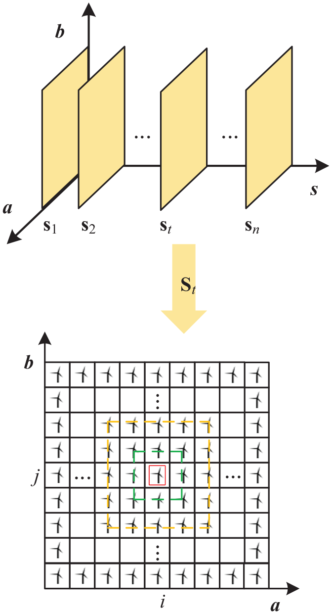
3-D spatiotemporal sequence and SWSM.

In SWSM, it is assumed that the WT located at (i, j) is a typical WT, and the surrounding WTs of the typical WT are defined as the first-order neighborhood and marked as neighborhood-I; the WTs adjacent to the first-order neighborhood are defined as the second-order which is identified as Neighborhood-||, and so on. The spatial position sequence of the target range area can be determined.

A wind farm A in northeast China was selected for the study (see appendix for topographic map of wind farm A), and the wind speed fluctuations of typical turbines are shown in Figure 2. A randomly selected 9 × 9 fleet in A was used to construct the SWSM, and the wind speed correlationγ(V) between typical turbines and each neighborhood was calculated using the measured data in August 2019 for analysis, and the results are shown in Table 1.

Figure 2.

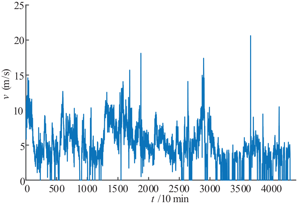
Target wind turbine wind speed fluctuation chart.

Table 1.

Correlation coefficient γ for each.

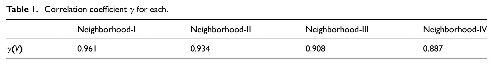
	Neighborhood-I	Neighborhood-II	Neighborhood-III	Neighborhood-IV
γ ( V )	0.961	0.934	0.908	0.887

In Table 1, the first-order neighborhood has the highest correlation with typical WT, and the second-order is the second. The higher the neighborhood order, the smaller the correlation. The degree of spatial correlation of the wind speed sequence depends on the distance between the typical WT and its neighborhood. The further away from the typical WT, the lower the spatial correlation.

Therefore, the reconstruction rule of the WT matrix in this paper is to select the neighborhood-I of the typical WT and the wind speed sequence of the row and column as the matrix information to reconstruct the WT matrix.

Wind speed-power correlation calculation

The purpose of wind speed prediction for wind farms is to predict wind power, thereby improving the flexibility of new energy grid connection. Therefore, the gray correlation is used to analyze the correlation between the wind speed and wind power of different WTs, so as to select a more representative WT as a typical WT. Calculate the wind speed-power correlation γ(V–P) of each WT in the wind farm A, take the wind speed sequence V as the reference sequence, and the power sequence P as the comparison sequence. The results are shown in Figure 3.

Figure 3.

Correlation coefficient γ(V–P) of each wind turbine.

In Figure 3, the γ(V–P) correlation is mainly concentrated in the range of [80%, 90%], and the corresponding WTs are located in the cluster array, indicating that these WTs are greatly affected by the wake effect, resulting in a low correlation. A few WTs are located at the edge of the array, which is less affected by the wake of the incoming wind and has a higher correlation.

Timing-controlled spatial association optimization

In view of the fact that each WT in the WT array has different spatial correlation, if the spatial correlation is considered for wind speed prediction, it needs to be extended to the global through the local features, which leads to the increased complexity of extracting the spatial characteristics of the wind farm. To solve this problem, combining the γ(V–P) and the γ(V), this paper uses TSAO to select typical WT, and then reconstruct the wind turbine array according to the specified rules, thereby reducing the complexity of spatial information extraction and improving the wind speed prediction efficiency.

The idea of selecting typical WT based on the spatial control optimization algorithm based on timing control is a new optimization algorithm improved based on the population optimization algorithm. It has a strong global search ability, can search without finding the regional scale and find a global optimal that overcomes the local optimal solution. Therefore, TSAO is more suitable for optimizing the WT sequence in the wind farm.

Combined with the geographic information of the wind farm, it is regarded as the survival forest of animal populations. The forest trees represent the location of each WT. To conduct a search, the mathematical model can be expressed as:

\begin{matrix} min F (v^{(d)}) = ψ \cdot {(γ_{V} (v^{(d)}))}^{- 1} + (1 - ψ) \cdot {(γ_{V - P} (v^{(d)}))}^{- 1} \\ {\begin{matrix} V = [v_{ij}], i, j \in D 且 i, j = 1, 2, \cdot \cdot \cdot, 5 \\ L_{ij} \leq v_{ij} \leq U_{ij} \end{matrix} \end{matrix}

(7)

Where: v is a D-dimensional space variable matrix, where D = 2; Gen is a population algebra and ψ is a weight coefficient, L_ij and U_ij are the upper and lower limits of the spatial variable v_ij, respectively.

The main steps are as follows:

(1) Initialization. Set the number of beetles in the population N, the number of pioneers N′, the upper limit U of the preferred matrix, the lower limit L and the termination standard End.

(2) Send pioneer particles to search. N′ particles are randomly placed in a hyper-volume equal to the global search space, and the best position vector v ⁽⁰⁾ is found. Each vanguard particle of the first population v_z⁽⁰⁾ randomly enters the global search area:

v_{z}^{(0)} = RST (L, U, D, N'), z = 1, 2, \dots, N'

(8)

where: L =[L₁,L₂,…,L_D], U =[U₁,U₂,…,U_D], and z=1,2,…, N′, RST is a random sampling technique.

(3) New hypervolume selection mode. All new particles are searched in the search space for better solutions to create their own children. Based on the selected new hypervolume selection mode, a search area is created around the position where the particles are generated. For each mode, an appropriately selected mode factor (χ) is used to achieve the definition of the region and represent the parameters of the TSAO. According to each mode, N′ new pioneer particles are randomly located in this search area through RST:

v_{z}^{(1)} = RST (l^{(1)}, u^{(1)}, D, N')

(9)

Where l and u are subsets of L and U , respectively, and the value range is [l_i⁽¹⁾, u_i⁽¹⁾]∈[v_birth,i⁽¹⁾(1−χ), v_birth,ii⁽¹⁾(1+χ)]

(4) Update the population position. In this step, the brooding position is updated and the past position is discarded. And the beetles of the past have become extinct, and the new place has become the birthplace of a new generation. Select the hypervolume mode for the new population based on the previously described rules. Repeat steps (3), (4) until the termination criteria for TSAO are met.

(5) In order to obtain the optimal target selection that fits the actual situation, the time control model is embedded according to the optimal probability. When the time node is ϑ, comprehensively sort the goals obtained by each optimization to get the goal with the highest probability.

P_{max} = \frac{V_{ij}^{*}}{ϑ} \cdot 100 %

(10)

Where: V_ij^* is the target with the highest number of times selected.

Reconstruct the SWSM according to the TSAO optimization results, generate a new SWSM^* and input it to the convolutional memory network to improve the spatial feature extraction efficiency and multi-step prediction accuracy.

Convolutional memory network

Most current wind speed prediction methods have limited prediction accuracy due to ignoring spatial feature information, and most shallow learning algorithms cannot mine the deep features hidden in the original data. In response to this problem, this paper uses the CMN model to predict the reconstructed wind speed matrix, and can directly input multiple SWSM^* to the CMN without expanding the two-dimensional spatial information into a one-dimensional sequence, to avoid the loss of spatial information. The prediction process can be divided into two parts. First, spatial feature extraction is performed to achieve dimensional compression and deep feature mining, and then the memory unit is used to predict the wind speed in multiple steps. The specific structure is shown in Figure 4.

Figure 4.

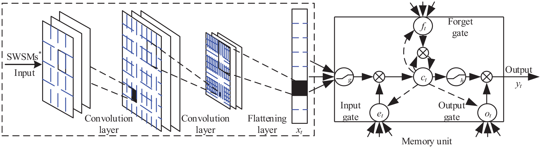
CMN structure diagram.

Spatial feature extraction

The spatial extraction part of CMN overwrites the input SWSM^* through multiple convolution kernels in the input layer and performs feature extraction to form a new feature matrix. And then performs feature extraction of the feature matrix layer by layer through the new convolution kernel until the generated features graph can be expanded into the required feature sequence through the fully connected layer.

In the CMN architecture, there is no connection between neurons in the same layer. In addition, weight sharing technology is used between neurons in different network layers to simplify the feedforward and backward propagation processes. Specifically, the feature map in the previous (l−1) layer is convolved with the shared weights, and then the first layer with several output feature maps is generated through the defined activation function, as shown below

x_{J}^{l} = h (\sum_{I \in N_{M}} v_{I}^{l - 1} \otimes w_{IJ}^{l} + g_{J}^{l})

(11)

Where: h is the activation function, ⊗ is the symbol of the convolution operation, v^l_J is the Jth feature maps of the lth layer; $w_{IJ}^{1}$ is the convolution kernel matrix, g^l_J is the bias matrix, N_M is the set of input feature maps.

Through the data extraction and feature extraction of SWSM^* by the space extraction part, the key data and association rules implied in the space features can be obtained to improve the accuracy of wind speed prediction.

Multi-step wind speed prediction

Each memory prediction unit has a memory cell, and its state at time t is recorded as c_t. The reading and modification of c_t are realized through the control of input gate e_t, forget gate f_t and output gate o_t. f_t receives the current state x_t and the hidden layer state y_t−1 at the previous moment. And the previously received state is activated with the activation function σ, in order to make the output value of the forget gate is between [0, 1]. The information indicates the previous state is completely discarded when the output is 0. The previous state information is all retained when the output is 1. Input of input gate after nonlinear transformation and the output of the forget gate are stacked to obtain the updated memory cell state c_t. Finally, the output gate obtains the output y_t according to the c_t dynamic control after the nonlinear function operation.

f_{t} = σ (W_{xf} x_{t} + W_{yf} y_{t - 1} + W_{cf} c_{t - 1} + r_{f})

(12)

e_{t} = σ (W_{xe} x_{t} + W_{ye} y_{t - 1} + W_{ce} c_{t - 1} + r_{e})

(13)

c_{t} = f_{t} c_{t - 1} + e_{t} \tanh (W_{xc} x_{t} + W_{yc} y_{t - 1} + r_{c})

(14)

o_{t} = σ (W_{xo} x_{t} + W_{yo} y_{t - 1} + W_{co} c_{t - 1} + r_{o})

(15)

y_{t} = o_{t} \tanh (c_{t})

(16)

Where: W_xf, W_xc, W_xe, and W_xo are the weight matrix connecting the input signal x_t, W_yf, W_yc, W_yo, and W_ye are the weight matrix connecting the hidden layer output signal y_t, W_ce, W_cf, W_co are diagonal matrices that connect the neuron activation function output vector c_t and the gate function, r_e, r_c, r_f, and r_o are offset parameters, σ is an activation function, usually a tanh or sigmoid function.

Wind speed prediction and evaluation based on spatial correlation

The specific process of the multi-step real-time combined wind speed prediction method based on spatial correlation is shown in Figure 5:

Figure 5.

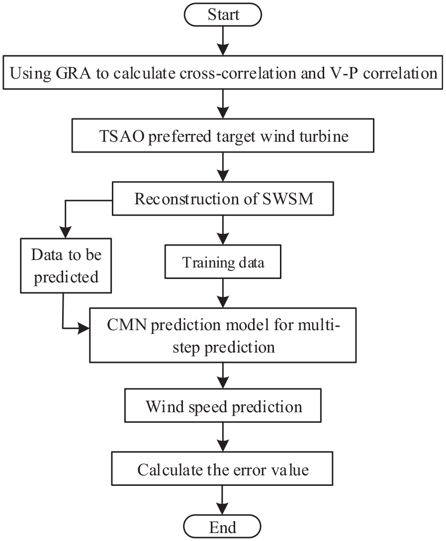
Wind speed combination prediction process.

When evaluating the prediction results, select the average absolute percentage error sensitivity ε₁, the root mean square error sensitivity ε₂ and the daily average prediction plan curve accuracy rate ε₃, and construct a multi-location, multi-step wind speed prediction evaluation index considering the spatial and temporal correlation:

ε_{1} (k) = \sqrt{\frac{\sum_{i = 1}^{a} \sum_{j = 1}^{b} \sqrt{\frac{1}{| N_{1} |} \sum_{t \in N} {(x {(i, j)}_{t + k} - y {(i, j)}_{t + k})}^{2}}}{a \times b}}

(17)

ε_{2} (k) = \frac{1}{a \times b} \sum_{i = 1}^{a} \sum_{j = 1}^{b} \frac{1}{| N_{1} |} \sum_{t \in N} \frac{| y {(i, j)}_{t + k} - v {(i, j)}_{t + k} |}{| v {(i, j)}_{t + k} |}

(18)

ε_{3} = {1 - \sqrt{\frac{1}{6} {\sum_{k = 1}^{6} [\frac{\sum_{i = 1}^{a} \sum_{j = 1}^{b} (y_{i j} (t + k) - v_{i j} (t + k))}{N_{2}}]}^{2}}}

(19)

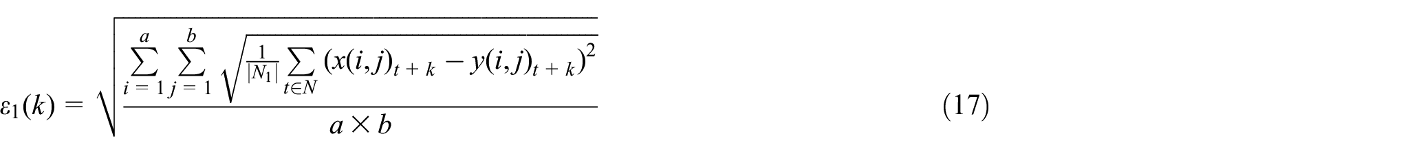
Where: k is the predicted step length, v is the measured wind speed value, y is the predicted wind speed value, a, b are the number of rows and columns in the wind farm array, N₁ is the set of test sample prediction time, N₂ is the total number of WT.

Study simulation

Select the WT layout information of Northeast wind farm A and make predictions based on the actual measured data of August 2019.

Design GRA-TSAO-CMN combined forecasting method for multi-step real-time wind speed forecasting, set basic parameters of TSAO N = 25, N′ = 5, g = 50, ϑ = 9. The prediction part of the CMN needs to determine the number of time steps of the input layer, that is, considering the length of the historical sequence, it will affect the calculation complexity and prediction accuracy of the model. If the number of steps is too large, the prediction performance of the model will be reduced, and if it is too small, the prediction error sensitivity will be larger. Jinfu et al. (2019) and Chen and Peng (2020) select input steps of 15 and 20 respectively. In this paper, we try to choose step 18 between 15 and 20 as the best, that is, the historical data at the time before the input 18 is used for prediction. The feature extraction part uses a three-layer structure, the first layer is set to have 15@3 × 3 convolution kernels, the second layer convolution layer uses 25@3 × 3 convolution kernels, and the third layer is fully connected layer, the two-dimensional features output by the convolution layer are expanded into a one-dimensional vector input prediction part.

Optimization of WT position based on GRA-TSAO

In order to avoid the particularity of WT location optimization, nine times within 1 month are randomly selected to use TSAO to represent the WT optimally. The size of the search matrix MATRIX’ is defined as 5 × 5. The WT array in the wind farm A is divided into area^I–area^VIII according to the number of rows from north to south, and area₁–area₁₈ according to the number of columns from west to east. Initialize the WT distribution matrix, the matrix element is the number of each WT, and the position of the uninstalled WT is 0. The results are shown in Table 2.

Table 2.

Preferred WT position ranking results.

		γ(V) best	γ(V) second best	γ(V-P) best	γ(V-P) second best	TSAO preferred
August first 0: 00	Typical WT	34#	50#	6#	24#	33#
August first 0: 00	SWSM	area^II₁₄	area^II₁₃	area^I₁₃	area^II₁₃	area^II₁₃
August first 9: 00	Typical WT	115#	96#	36#	5#	96#
August first 9: 00	SWSM	Area^VI₆	area^V₅	Area^II₁₆	area^I₁₃	area^V₅
August first 14: 00	Typical WT	58#	60#	12#	14#	59#
August first 14: 00	SWSM	area^IV₆	area^IV₇	area^I₂	area^I₄	area^IV₆
August 15th 0: 00	Typical WT	67#	84#	88#	69#	85#
August 15th 0: 00	SWSM	area^III₁₅	area^III₁₄	area^III₁₇	area^III₁₆	area^III₁₄
August 15th 9: 00	Typical WT	123#	140#	125#	157#	122#
August 15th 9: 00	SWSM	Area^VI₁₃	area^VII₁₆	area^VIII₁₈	area^VIII₁₈	area^VI₁₅
August 15th 14: 00	Typical WT	92#	76#	122#	105#	95#
August 15th 14: 00	SWSM	area^V₇	Area^IV₉	area^VI₁₃	area^V₁₂	area^V₅
August 30th 0: 00	Typical WT	95#	74#	124#	141#	95#
August 30th 0: 00	SWSM	area^V₅	Area^IV₇	area^VI₁₄	area^VII₁₃	area^V₅
August 30th 9: 00	Typical WT	161#	132#	168#	178#	165#
August 30th 9: 00	SWSM	area^VI₉	area^VI₁₀	area^VII₃	area^VIII₁₃	area^VIII₁₀
August 30th 14: 00	Typical WT	129#	95#	144#	148#	95#
August 30th 14: 00	SWSM	area^VI₇	area^V₅	area^VI₄	area^VI₇	area^V₅

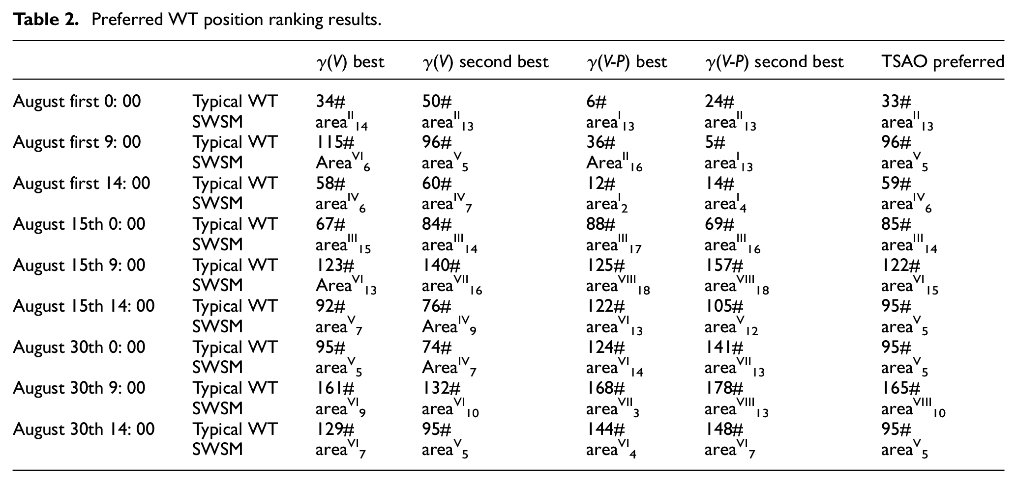
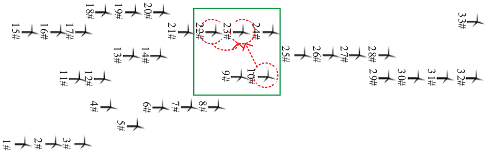
Considering that γ(V) is affected by the wind speed difference between the two WTs, the smaller the wind speed difference, the greater the degree of correlation, so it is necessary to avoid the zero-filling WT first when selecting SWSM. At the same time, the WT’s γ(V–P) that is not affected by the wake effect is higher, so TSAO defaults to prefer the WT coming from the edge of the wind farm. Therefore, in the optimization, the heuristic rules of weighted synthesis γ(V) and γ(V–P) are introduced. According to the results of the nine preferred rankings of TSAO in Table 2, the matrix area^V₉ is the final WT matrix. On this basis, five pioneer animals (N′) were selected in area^V₉ to sort the WTs again, and the 95# WT was obtained as a typical WT, as shown in Figure 6. The optimized results are reconstructed according to the WT matrix reconstruction rule in 1.2 to obtain a new spatial wind speed matrix SWSM^*.

Figure 6.

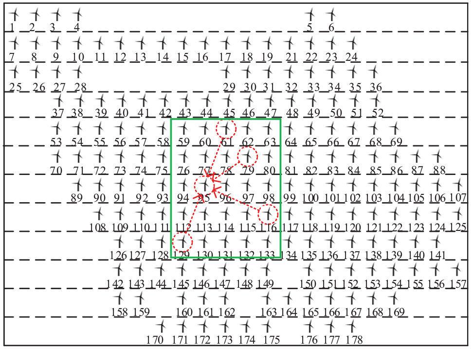
The result of TSAO.

Choose different combination methods for multi-step prediction to verify the effectiveness of TSAO. Among them, Method 1 is TSAO-CMN and Method 2 is CMN. The prediction results are shown in Table 3.

Table 3.

Contrast of prediction results of different methods.

k	Method 1			Method 2
	ε₁ (m/seconds)	ε₂ (%)	ε₃ (%)	ε₁ (m/seconds)	ε₂ (%)	ε₃ (%)
1	0.33	4.53	93.58	0.31	4.48	93.67
2	0.45	5.27	93.32	0.38	5.21	93.36
3	0.52	6.18	92.84	0.50	6.17	92.87
4	0.60	7.42	91.27	0.59	7.49	91.18
5	0.71	8.53	89.17	0.71	8.38	89.53
6	0.82	9.41	86.93	0.80	9.27	87.02

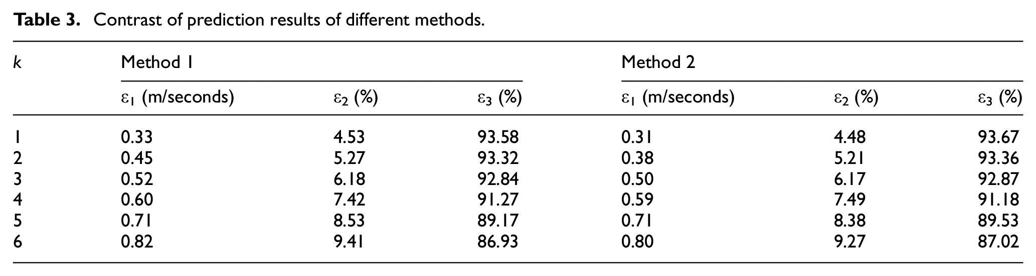
Both methods in Table 3 can effectively predict the wind speed of the WT array at multiple times. The training duration of Method 1 is 309.87 second, and the training duration of Method 2 is 467.15 second. The prediction efficiency is improved by 33.7%. It shows that the optimal reconstruction of the WT array by TSAO can significantly improve the calculation efficiency of the prediction model. From the perspective of prediction accuracy, Method 1 ignores the wind speed information of the higher-order neighborhood, which leads to a slight decrease in prediction accuracy. Among them, the maximum decrease of ε₁ is 0.07 m/s and the lowest is 0. It can be seen from this that Method 1 has higher prediction accuracy while improving prediction efficiency.

Wind turbine prediction accuracy analysis

The sampling interval of the measured data is 10 minutes. The monthly wind speed data constitutes 4320 SWSMs. The first 80% of the wind speed samples are used to train the combined wind speed model, and the second 20% of the wind speed is predicted. The SWSMs in the training set and test set are reconstructed and input to the CMN for training and prediction. To illustrate the effectiveness of CMN, six consecutive time points in the prediction set are randomly selected, and ultra-short-term wind speed prediction of 10 min–1 hour (i.e. 1–6 step prediction). And compared with persistence method (PR), autoregressive integral moving average (ARIMA) and BP neural network. PR directly uses the measured value of the current moment as the predicted value of the next moment; BP uses a single hidden layer network structure, the activation function is a sigmoid function, the learning rate is 0.01, the maximum number of iterations is 100, and the number of hidden layer neurons 33; ARIMA uses the ARIMA (0, 1, 1) model for training and prediction. The prediction results of different numbered WTs are shown in Figures 7 to 10.

Figure 7.

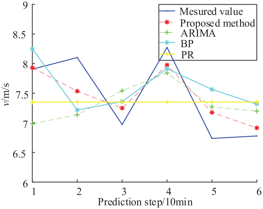
Comparison of prediction results of 95# wind turbine.

Figure 8.

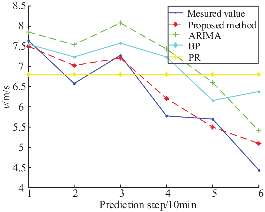
Comparison of prediction results of 79# wind turbine.

Figure 9.

Comparison of prediction results of 129# wind turbine.

Figure 10.

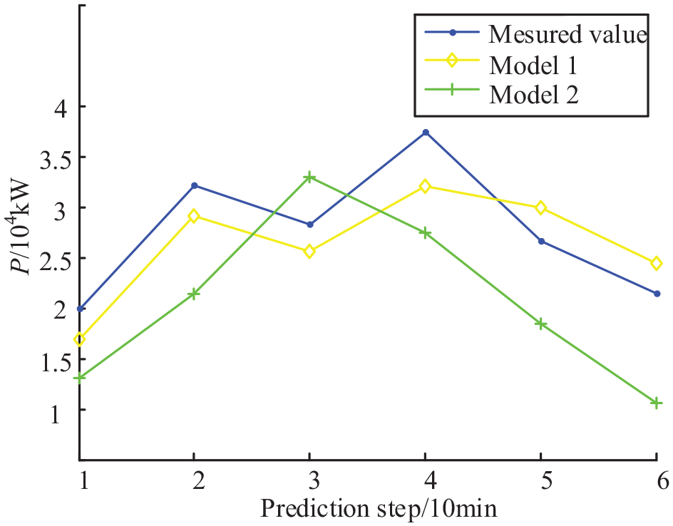
Contrast of array wind power prediction.

According to the prediction results of different WTs, the prediction results of the four methods can all meet the actual wind speed fluctuation to a certain extent. Among them, PR has a low prediction accuracy due to its single prediction structure. ARIMA and BP neural networks cannot directly input spatio-temporal data, but need to expand the spatial two-dimensional information into one dimension first. In this process, a lot of spatial related information will be lost, resulting in a large deviation between the prediction results and the actual. Relatively speaking, the method proposed in this paper can not only directly input three-dimensional spatio-temporal information, mine hidden deep features in spatial data and the correlation of various spatial positions, to avoid the decline in prediction accuracy due to ignoring spatial information, but also have a relatively higher random fluctuation of wind speed. With a good fitting effect, its error back propagation training algorithm can also effectively reduce the prediction error, so the CMN model can achieve a more accurate prediction effect.

The forecast time of different methods is shown in Table 4. In terms of prediction efficiency, as the method in this paper reduces the spatial complexity of the input wind speed matrix by preferentially reconstructing the spatial wind speed matrix through TSAO, the prediction time of CMN is reduced and the prediction efficiency is improved. In order to further explain the prediction effect of the method in this paper, an error sensitivity analysis is performed on the WT array. The prediction error sensitivity of each method are shown in Table 5.

Table 4.

Time complexity of different methods.

	TSAO-CMN	BP	ARIMA
t (seconds)	309.87	513.12	437.35

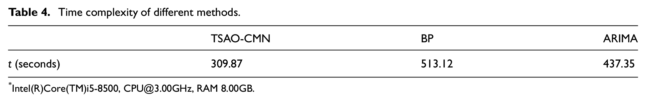
Intel(R)Core(TM)i5-8500, CPU@3.00GHz, RAM 8.00GB.

Table 5.

Contrast of prediction errors of different algorithms.

k	ε₁ (m/seconds)				ε₂ (%)
	TSAO-CMN	BP	ARIMA	PR	TSAO-CMN	BP	ARIMA	PR
1	0.33	0.57	0.59	0.74	4.53	7.04	8.87	9.68
2	0.45	0.68	0.69	0.82	5.27	8.75	9.13	9.94
3	0.52	0.79	0.76	0.94	6.18	10.89	10.87	11.72
4	0.60	0.88	0.87	1.05	7.42	12.85	12.04	12.97
5	0.71	1.01	0.99	1.15	8.53	13.66	13.55	14.26
6	0.82	1.17	1.11	1.31	9.41	15.96	14.96	16.87

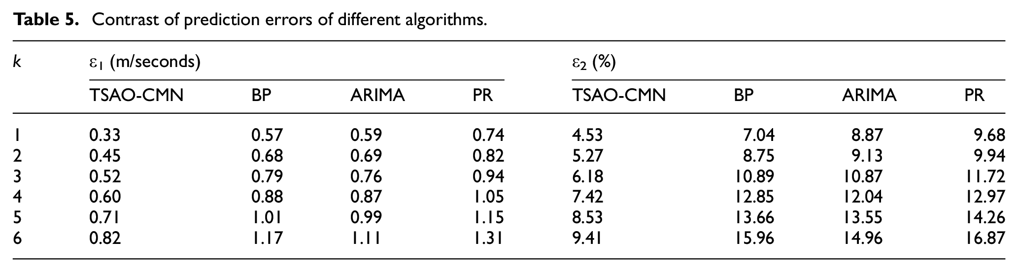
The results show that the prediction performance of PR is significantly weaker than the other three methods, and as the prediction step size increases, its disadvantage becomes more obvious. The six-step average error sensitivity ε₁ for the method in this paper is 0.57 m/s and sensitivity ε₂ is 6.89%. The average error sensitivity ε₁ of the BP neural network is 0.85 m/s and the sensitivity ε₂ is 11.53%, ARIMA’s ε₁ is 0.84 m/s and ε₂ is 11.57%. Therefore, in the overall average performance and the ability to control individual errors, the method in this paper has a good performance, which benefits from the ability of CMN to choose to remember or forget historical wind speed information during the training process. Its feedback neural network structure improves its prediction accuracy compared with other algorithms. The root-mean-square error sensitivity of the BP neural network is smaller than that of ARIMA in 1–2 step prediction, and in 3–6 step prediction, the error sensitivity is larger than that of ARIMA, indicating that it is more suitable for smaller step prediction, such as single-step rolling prediction. On the other hand, due to the chaotic nature of the time series of wind speed, the error sensitivity of multi-step prediction increases with the time scale. This conclusion is consistent with the literature (Yang et al., 2019; Zhang et al., 2011).

Comparative analysis of wind power multi-step prediction

In order to verify the applicability of the model and meet the needs of the project, the wind power of the obtained wind speed is further converted to realize the ultra-short-term wind power array wind power forecast. Select the equivalent wind energy with higher precision and use the coefficient method (Chao and Benshuang, 2017) to predict the wind power.

Since the wind farm A is relatively flat, the spatial distribution of the fan array units is basically the same, so all units are selected as a group, and the equivalent wind energy utilization coefficient is calculated according to the following formula:

P_{Σ} = \sum_{j = 1}^{b} \sum_{i = 1}^{a} P_{i, j} = \sum_{e = 1}^{N_{2}} \frac{1}{2} ρ N_{2} s C_{p . e} v_{max}^{3}

(20)

Where: P_Σ is the total power predicted by the array; P_i,j are the measured power values; s is the sweep area of the blade; C_p,e is the equivalent wind energy utilization factor; v_max is the maximum wind speed in the array.

The C_p,e is calculated by the above formula to be 0.1513. Based on this coefficient, the wind power of the selected aircraft group is predicted.

In Figure 10, Model 1 is the predicted wind power value obtained based on the model in this paper, and the wind power is further converted. Model 2 is used to directly predict the wind power value of the model in this paper.

It can be seen from Figure 11 and Table 6 that the wind power prediction accuracy of Model 1 is higher than that of Model 2 when it is not synchronized, and the accuracy advantage is obvious. This is because there are a large number of zero points in the wind power prediction, that is, the wind speed is less than the cut-in wind speed point, which causes the accuracy of the model to predict the wind speed is higher than the wind power prediction. When predicting the wind power according to the equivalent wind energy using the coefficient method for wind power prediction, the points that do not meet the power generation standard can be reset to zero, and the remaining points are converted to wind power prediction, thus significantly improving the prediction accuracy. At the same time, the wind power forecasting time has increased by 10.79 seconds relative to the direct forecasting method, which meets the requirements of the forecasting standard. Relatively speaking, although Model 1 is slightly more complicated in the prediction step, it has a greater advantage in accuracy and has more practical significance.

Figure 11.

Wind farm B optimization results.

Table 6.

Comparison of the error sensitivity of different methods.

k	ε₁ (m/seconds)v		ε₂(%)
	Model 1	Model 2	Model 1	Model 2
1	0.651	1.001	7.072	9.326
2	0.873	1.393	8.559	10.075
3	1.318	1.904	9.736	14.259
4	1.580	2.813	12.169	15.837
5	2.097	3.230	14.341	18.106
6	2.529	3.808	16.624	19.794

Generalized verification

In order to avoid the influence of the latitude and longitude of the selected area and the particularity of the climate, a wind farm B (see Appendix for the topographic map) of China Southern Power Grid was selected to verify the generalization ability of the proposed method. Because the selected area is mountainous terrain, it is quite different from the centralized large-scale wind farm in the Northeast Plain area. This wind farm is a small-scale fleet built according to the trend of the ridge.

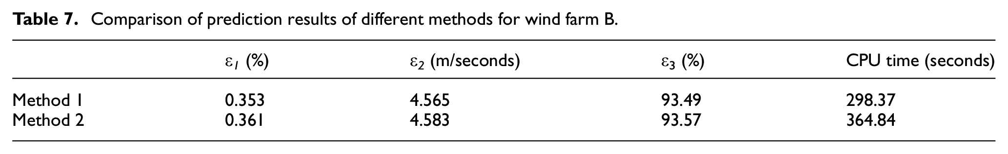
According to the terrain and scale of the wind farm B, set the basic parameters of TSAO N = 9, N′ = 3, g = 30. The optimal results based on γ(V) and γ(V–P) are shown in Figure 11. Reconstruct, extract and predict the selected SWSM, and compare the results with different methods. The results are shown in Tables 7 and 8.

Table 7.

Comparison of prediction results of different methods for wind farm B.

	ε₁ (%)	ε₂ (m/seconds)	ε₃ (%)	CPU time (seconds)
Method 1	0.353	4.565	93.49	298.37
Method 2	0.361	4.583	93.57	364.84

Table 8.

Contrast of wind speed prediction errors of different algorithms for wind farm B.

k	ε₁ (%)				ε₂ (m/seconds)
	CMN	BP	ARIMA	PR	CMN	BP	ARIMA	PR
1	0.33	0.45	0.49	0.74	4.53	8.04	7.87	9.68
2	0.45	0.57	0.61	0.82	5.27	8.75	9.13	9.94
3	0.52	0.79	0.76	0.94	6.18	9.89	10.87	10.72
4	0.60	0.88	0.87	1.05	7.42	10.85	11.04	11.97
5	0.71	1.01	0.99	1.15	8.53	11.66	12.55	13.26
6	0.82	1.17	1.11	1.31	9.41	12.96	13.96	14.87

The distribution of WTs in wind farm B has a large dispersion, which reduces the wind speed correlation, resulting in covering most of the spatial feature information of WTs during feature extraction. Therefore, the error sensitivity of the two methods in Table 7 are relatively close. It can be seen from Table 8 that the prediction results of the proposed method can more accurately reflect the change trend of wind speed than the comparative method, and further predict the wind power of the wind farm. The results are shown in Figure 12.

Figure 12.

Wind farm B array wind power prediction comparison.

It can be seen from Figure 12 that the forecasting indicators of Model 1 all meet the standard requirements, which verifies that this method can not only achieve good prediction results for large-scale wind farms in the plain, but also apply to decentralized wind farms in hilly areas. It has strong applicability and generalization ability.

Conclusion

Based on the spatial correlation of wind turbines, a combined multi-step prediction method for wind speed and wind power of wind farms is proposed, and the following innovative conclusions are drawn:

Based on the gray correlation analysis results of the wind farm array wind turbines, the time-control spatial association optimization is used to optimize the ranking of typical wind turbines and wind turbine matrices, and the spatial wind speed matrix is reconstructed, which can reduce the complexity of key information extraction and improve the operation efficiency. Simulation results show that adding this step improves computing efficiency by 33.7%.

Input the reconstructed spatial wind speed matrix into the convolutional memory network for spatial feature extraction and multi-step prediction. Considering the spatial correlation can avoid the prediction accuracy degradation caused by the lack of peripheral information. Feedback neural network can effectively reduce the prediction error. By constructing a combined prediction method to predict wind speed and wind power for the actual wind field, where the root mean square error of wind speed prediction in this paper is 0.57 m/s and the average absolute percentage error is 6.89%, verifying the higher accuracy of the proposed method compared to existing methods. The applicability of the proposed method is further verified by the prediction results of wind field B.

Footnotes

Appendix

Declaration of conflicting interests

The author(s) declared no potential conflicts of interest with respect to the research, authorship, and/or publication of this article.

Funding

The author(s) received no financial support for the research, authorship, and/or publication of this article.

ORCID iD

Dian Wang

References

Chao

Benshuang

(2017) Research on power model of large-scale wind farm based on measured data. Power System Technology 41(08): 2625–2631.

Chao

Qide

Guowei

, et al. (2018) COA-SVR short-term wind speed hybrid prediction model based on recursive quantitative analysis. Power System Technology 42(8): 2373–2381 (in Chinese).

Chen

Peng

(2020) Wind speed forecasts of multiple wind turbines in a wind farm based on integration model built by convolutional neural network and simple recurrent unit. Journal of Electrical Engineering and Technology. Epub ahead of print 22 April 2020. DOI: 10.19595/j.cnki.1000-6753.tces.191715.

Jin

Jizhong

, et al. (2019) Simulation of wind power output sequence based on spatiotemporal autoregressive moving average model. Automation of Electric Power Systems 43(03): 101–109.

Jinfu

Qiaomu

Dongyuan

, et al. (2019) Multi-position multi-step wind speed prediction model using space-time correlation. Proceedings of the CSEE 39(07): 2093–2106.

Kallioras

Lagaros

Avtzis

(2018) Pity beetle algorithm-A new metaheuristic inspired by the behavior of bark beetles. Advances in Engineering Software 121: 147–166.

Ling

Zeqi

Yue

(2019) Multi-step wind speed prediction model based on LPF-VMD and KELM. Power System Technology 43(12): 4461–4467.

Lingling

Yahui

Xiaoyue

, et al. (2014) Short-term prediction of wind power based on combined model. Journal of Electric Engineering 29(S1): 475–448.

Liu

, et al. (2019) Smart wind speed deep learning based multi-step forecasting model using singular spectrum analysis, convolutional Gated Recurrent Unit network and Support Vector Regression. Renewable Energy, 143: 842–854.

10.

Mao

Binyang

(2017) Research on wind power real-time prediction based on quantified index of probability distribution and grey correlation decision. Proceedings of the CSEE 37(24): 7099–7107.

11.

Ning

Yusheng

Jie

, et al. (2017) Ultra-short-term wind speed prediction using spatial correlation. Automation of Electric Power Systems 41(12): 124–130.

12.

Ruili

Zhizhong

Ruiye

, et al. (2017) Wind speed and wind power prediction of wind farm based on wavelet packet decomposition and improved Elman neural network. Transactions of China Electrotechnical Society 32(21): 103–111.

13.

Schicker

Papazek

Kann

, et al. (2017) Short-range wind speed predictions for complex terrain using an interval-artificial neural network. Energy Procedia 125: 199–206.

14.

Shouxiang

Lei

, et al. (2016) Wind speed forecasting based on the hybrid ensemble empirical mode decomposition and GA-BP neural network. Renewable Energy 94: 629–636.

15.

Shuanglei

Weisheng

Chun

, et al. (2011) Short term wind speed prediction based on physical principle. Acta Energiae Solaris Sinica 32(5): 611–616.

16.

Wang

, et al. (2017) Deep learning based ensemble approach for probabilistic wind power forecasting. Applied Energy 188: 56–70.

17.

Xiaoling

Rong

Hua

, et al. (2017) Short-term wind speed correction for wind farms based on WRF model and PSO-LSSVM. Power System Protection and Control 22: 53–59.

18.

Yang

Zhang

Cui

, et al. (2019) The impact of wind farmspatial heterogeneity and variability on short-term wind power forecast errors. Journal of Renewable and Sustainable Energy 11: 033304.

19.

Zhang

Zou

Zheng

(2011) Ultra-short term wind power prediction model based on modified grey model method for power control in wind farm. Wind Engineering 35: 55–67.