High resolution wind resource assessment method based on mesoscale atmospheric model and CFD technology

Abstract

The evaluation results of wind energy resources directly affect the economic benefits and healthy development of wind farms. Therefore, a high-resolution wind resource assessment method for wind farms based on mesoscale atmospheric model and CFD technology is studied to accurately simulate relevant data of wind resources and improve the assessment effect. The mesoscale WRF numerical model is used to solve the regional data of wind farms and obtain the mesoscale meteorological analysis data. According to the solution results of the mesoscale atmospheric model, the wind speed profile is established, the boundary conditions and initial conditions are extracted, and the CFD micro scale model is input to obtain the wind speed and wind speed frequency at the height of the fan impeller. In order to improve the accuracy of numerical simulation of micro scale CFD model, the large eddy simulation method is used to simulate the operation of wind farms. Complete theoretical power generation evaluation based on wind speed, wind speed frequency and generator power. The experimental results show that this method can accurately simulate wind resources and accurately evaluate the theoretical power generation of wind farms. The wind farm is rated as Level 3, and the wind frequency is mainly between 4 and 10 m/s. This method can ensure that the wind farm can generate electricity all year round without damaging the wind speed.

Keywords

The mesoscale atmospheric model CFD technology wind farm high resolution wind resource assessment

Introduction

The key part of wind farm construction is wind resource evaluation, which is of great significance to promote the upgrading of domestic wind power industry. Accurate results of resource analysis can be obtained in the assessment of industrial wind resources, providing high-quality consulting results and design schemes for government departments and investment enterprises, and promoting the healthy development of wind power (Han et al., 2020; Wang et al., 2019a; Ye et al., 2019). At present, the most serious problem existing in the wind power project is that there is no wind measurement data in the field before the project is established (Yu et al., 2019), and the wind measurement time of the wind measurement tower cannot meet the requirements of the Wind Power Farm Wind Energy Resource Assessment Methods and the Wind Power Plant Design Code for 1 year. Whether the wind resource assessment is accurate or not will directly affect the rate of return on investment of the wind power project and the declared electricity price during the operation period of 20 years. The average wind speed at hub height is 0.1 m/s per phase, and the annual equivalent utilization hours of wind turbine can reach 100 hours. The accuracy of wind resources and models has a significant impact on wind resources assessment and generation calculations (Li et al., 2020a). P Dur á n compared the simulation results of the newly developed mesoscale microscale coupling method for steady-state computational fluid dynamics (CFD) models with the mesoscale and independent microscale simulations at five locations. The coupling method uses the average wind speed field and potential temperature field simulated by the weather research and prediction model as the boundary and initial conditions of the CFD model. MB Ozkan applies the regional SHWIP to the potential power plant area, so that investors can obtain preliminary power forecasts, thus obtaining the wind potential of the area, without any financial costs of repeated measurement, and the calculated man hours can be ignored. W Nam proposed an alternative solution to predict the long-term wind resources of sites with seasonal and year-on-year changes, in which long-term reference data are not available. An analysis shows that complementary measurement related forecasting methods can be used because several data sets obtained in the short term are used to correct long-term wind resource data in a complementary manner. In addition, this method can be used to assess extreme wind speeds, which is one of the main factors affecting the site compliance assessment and the selection of appropriate wind turbine ratings according to IEC standards.

Li et al. (2000b), based on the idea of stepwise clustering analysis, created a downscaling model. The model is calibrated to obtain the best downscaling model. The wind resource assessment is completed by combining the climate model of Hadley Center. The experimental results show that the wind energy in the studied area increases in autumn and winter, and the wind energy in spring is relatively small, so the regional wind resource assessment can be completed effectively. Ma et al. fully considered the wind shear index and wind power density, and modeled the wind speed extrapolation model of hub height. They completed the wind resource assessment. Experimental results show that this method can effectively solve the problem of wind resource evaluation precision caused by wind shear index, and improve the evaluation precision of wind resource (Ma et al., 2020). Neither of the two methods is suitable for mountain wind farm, and there are some limitations in evaluating the wind resources of mountain wind farm. The result of the assessment will be a lot of uncertainty due to the complicated mountain flow of fluid, which will lead to a great error. Mesoscale atmospheric model and CFD technique have higher accuracy and reliability in wind resource assessment when wind farm planning lacks wind data. These technologies provide a strong basis for land conservation and project investment decisions (Liu et al., 2019). Therefore, this paper studies the wind farm high-resolution wind resource evaluation method based on mesoscale atmospheric model, namely CFD technology. The mesoscale WRF numerical model is used to solve the regional data of wind farms and obtain the mesoscale meteorological analysis data. The wind profile is established, the boundary conditions and initial conditions are extracted, and the micro scale CFD model is input. Start the micro scale CFD model for numerical simulation, and complete the wind energy resource evaluation of the wind farm. We verify the adaptability and accuracy of this method in complex mountain projects by comparing the difference between the method and the wind tower data. Provide data support and basis for future project construction.

High-resolution wind resource assessment method for wind farms

The wind resource assessment process based on the mesoscale atmospheric model and CFD technology is shown in Figure 1.

Figure 1.

Evaluation flowchart.

Specific steps are as follows:

Step 1: The mesoscale WRF numerical model is used to solve the data of wind farm region and obtain the mesoscale meteorological analysis data.

Step 2: According to the result of step 1, the wind profile is constructed, the boundary conditions and initial conditions are extracted, and the micro-scale CFD model is input.

Step 3: Start microscale CFD model to carry out numerical simulation and complete wind farm wind resource evaluation.

Mesoscale atmospheric model

The model chosen for the mesoscale model is WRF, and the values of such parameters as atmospheric boundary layer (ABL) and surface boundary layer (RSL) shall be analyzed when the model is solved. WRF is a new generation of weather and climate simulation system. The model has high accuracy, new scheme, and contains a variety of earth system processes. It is increasingly widely used in meteorology and related fields (meteorological services, agriculture and forestry, new energy, etc.). The boundary pressure value of the top floor is taken as 50 hPa. The integral step of the model solution is 90 seconds, the boundary condition update frequency is 6 hours, the running time is 2 years, and the starting time is 5 seconds. Three layer grid nesting scheme is adopted, and bidirectional feedback mode is adopted between adjacent nesting regions. The innermost nesting area has the smallest space range among the three nesting areas Arakawa-C grid is used in the horizontal direction of the model, and terrain following coordinate system is used in the vertical direction. The horizontal resolution of the grid points is 9 and 3 km respectively. Physical parameterization schemes include cloud microphysical scheme, cumulus convection scheme and planetary boundary layer scheme. The cloud microphysical scheme describes the formation, transformation, aggregation and growth of cloud particles and wind farm particles. This scheme can affect the conditions for the occurrence and development of the convection system by adjusting the structural characteristics of the temperature field and humidity field, thus affecting the process of the wind farm. The cumulus convection scheme focuses on the macro structural characteristics, thermal processes and evolution laws of cloud clusters and cloud systems as a whole. This scheme can compensate for the sub grid wind farm generated when the grid humidity does not reach the saturation humidity, so it has a greater impact on the wind farm results when simulating the convective wind farm process with stable stratification and neutral stratification characteristics. The planetary boundary layer scheme mainly describes the atmospheric motion in the lower troposphere. This scheme can affect the distribution characteristics of temperature, humidity and wind speed fields in the middle and upper troposphere by adjusting the vertical movement of the gas in the lower troposphere, thus affecting the results of wind farms. On the basis of existing research, the UN and WSM six cloud microphysical parameterization schemes that perform well in regional high-resolution wind farm process simulation and are widely used are selected. The values of RSL refer to Monin Obukhow simulation theory. The values of ABL refer to the TKE type structure of turbulent kinetic energy and the K-profile type of Richardson number.

Microscale CFD models

In order to improve the accuracy of numerical simulation of micro-scale CFD model, large eddy simulation method is selected to simulate the operation of wind farm. CHEN-KIM standard model was used for research. We introduce an actuator line model to simulate wind turbine blades to improve the accuracy of simulating the interaction between wind turbine blades and atmosphere (Ding et al., 2019; Wang et al., 2019b; Yu and Ke, 2020).

The numerical simulation of microscale CFD model is to solve the transient N-S equation, which needs to be filtered before the large eddy simulation control equation is obtained (Yao et al., 2019). The filtering function is as follows:

\bar{λ} (x) = \int_{D} λ (q') G (q, q') dq'

(1)

In formula (1), the flow variable is λ. The fluid solution domain is D. The filtering function is G. The flow characteristic data of initial wind farm is $q'$ .

The governing equations of LES after filtering are as follows:

{\begin{matrix} \frac{\partial \bar{v_{i}}}{\partial \bar{q_{i}}} = 0 \\ \frac{\partial \bar{v_{i}}}{\partial o} + \frac{\partial (\bar{v_{i}} \bar{v_{j}})}{\partial q_{j}} = - \frac{1}{ρ} \frac{\partial \bar{p}}{\partial q_{i}} + z \frac{\partial^{2} \bar{v_{i}}}{\partial q_{j} \partial q_{j}} + \frac{\partial τ_{ij}}{\partial q_{j}} + f_{i} \end{matrix}

(2)

In formula 2, the fluid density is ρ. The kinematic viscosity is z. The sub-lattice stress term is $τ_{ij}$ . The volume force is $f_{i}$ . The speed is $\bar{v_{i}}$ , $\bar{v_{j}}$ . Turbulent kinetic energy volume generation rate is $\bar{p}$ , resulting from shear force (Huang et al., 2020). The fluid temperature is o. The formula for $τ_{ij}$ is as follows:

τ_{ij} = \bar{v_{i}} \bar{v_{j}} - \bar{v_{i}} \bar{v_{j}}

(3)

$τ_{ij}$ is the momentum transport after filtering out small scale fluctuations and solvable scale turbulence. By establishing $τ_{ij}$ closed model, the N-S equation is calculated. Under the Boussinesq hypothesis, $τ_{ij}$ is required to:

τ_{ij} = - \frac{1}{3} τ_{kk} δ_{ij} = - 2 μ_{t} \bar{S_{ij}}

(4)

In formula (3), the sub-grid is τ. The symbolic function is $δ_{ij}$ . The stress homogeneity of τ is $τ_{kk}$ . τ turbulent viscosity is $μ_{t}$ . The stress tensor deformation rate is $\bar{S_{ij}}$ and the formula is as follows:

\bar{S_{ij}} = \frac{1}{2} (\frac{\partial \bar{v_{i}}}{\partial q_{j}} + \frac{\partial \bar{v_{j}}}{\partial q_{i}})

(5)

In the Smagorisky sub-grid model, the formula for $μ_{t}$ is as follows:

μ_{t} = L_{s}^{2} | \bar{S} |

(6)

In formula (6), $| \bar{S} | = \sqrt{2 \bar{S_{ij}} \bar{S_{ji}}}$ . The sub-grid scale mixing length is $L_{s}$ and the formula is as follows:

L_{s} = min (κ d, B_{s} V^{1 / 3})

(7)

In formula (7), the constant is κ. The distance is d. The Smagorisky constant is $B_{s}$ . The grid volume is V.

Within the actuating line model, the foliage is divided according to the principle of foliage, and the division direction is the direction of each actuating line (Zhang and Cheng, 2020). The angles of attack and chord lengths are α and c, and the formulas of lift and drag for each leaf element are as follows:

{\begin{matrix} dL = \frac{1}{2} B_{l} (α) ρ U_{rel}^{2} cdr \\ dD = \frac{1}{2} B_{d} (α) ρ U_{rel}^{2} cdr \end{matrix}

(8)

In formula (8), the lift and drag coefficients are $B_{l} (α)$ and $B_{d} (α)$ . The radial width is dr. The relative velocity of air and fan blade is $U_{rel}$ , the formula is as follows:

U_{rel} = \sqrt{U_{a}^{2} + {(Ω r + U_{t})}^{2}}

(9)

In formula (9), the axial and tangential velocities are $U_{a}$ and $U_{a}$ . The angular velocity of the wind wheel is $Ω$ .

The formula for force acting on leaf element per unit length is as follows:

f = (L, D) = \frac{1}{2} ρ U_{rel}^{2} c (B_{l} e_{L} + B_{d} e_{D})

(10)

In formula (10), the vectors of lift and resistance are $e_{L}$ and $e_{D}$ .

Using 3-D Gaussian mapping, the volume force generated by each driving element is reacted in the solution domain to avoid numerical turbulence in solving N-S equations (Jia et al., 2019). The formula for the Gaussian distribution function is as follows:

η_{ε} = \frac{1}{ε^{3} π^{3 / 2}} \exp [- {(\frac{r}{ε})}^{2}]

(11)

In formula (11), the distance between the grid point and the trigger point is r. The parameter is ω.

The formula of the volume force at $(x, y, z)$ position in the flow field is as follows:

f (x, y, z, t) = \sum_{i = 1}^{N} f (x, y, z, t) \frac{1}{ω^{3} π^{3 / 2}} \exp [- {(\frac{r_{i}}{ω})}^{2}]

(12)

In formula (12), the ith actuation point is $(x_{i}, y_{i}, z_{i})$ , and the total number of $(x_{i}, y_{i}, z_{i})$ is N.

Micro-scale CFD model is used to solve the wind condition information of the position of the hub-height of the wind turbine, and the wind condition information and generator power are combined to calculate the fan power. The formula is as follows:

AEP = \int_{0}^{A} P [{v'}_{h} (t)] dt

(13)

In formula (13), the generator power is $P [w_{h} (t)]$ . The interval time series is A. The position of hub height at each time point is $v'_{h} (t)$ .

Experiment analysis

Project overview

The experimental project relies on a mountain power plant in Ningxia. The wind farm has established 18 wind tower, showing north-south distribution. Among them, 11 wind measuring towers have 1-year observation data, and 7 wind measuring towers have only 6 months wind measuring data. At present, the mesoscale data of 18 wind measuring towers and the data of meteorological stations around the project are collected. The mesoscale data source is 3TIER numerical weather forecast model data. In this paper, the mesoscale model of wind farm is established by using 3TIER mesoscale data and the contemporaneous data of nearby reference weather stations. The precision of the mesoscale data model is 3 km. Subsequently, the micro-scale CFD model is established by CFD technology, and the precision of the micro-scale CFD model is 35 m. The reliability and feasibility of this method are proved by verifying and checking the method and the existing data. The scope of the project and the location of the wind tower are shown in Figure 2.

Figure 2.

Project scope and wind tower location.

As shown in Figure 2, 18 wind towers were built at the site of the project. The yellow logo for seven short-term wind tower, red logo for 11 long-term wind tower.

Model building

Large eddy simulation method is used to simulate the operation of wind farm. In order to improve the simulation accuracy of the interaction between wind turbine blades and the atmosphere, an actuator linear model is introduced to simulate the wind turbine blades. Based on the above methods, the micro scale CFD model of the wind farm is established, as shown in Figure 3.

Figure 3.

Wind farm microscale CFD model.

Wind resources assessment grade

Wind power density is the comprehensive index of wind resource in wind farm. According to the national standard, seven grades of wind resources are obtained. The grade table is shown in Table 1.

Table 1.

Wind power density class table.

Height	Index	Grade
Height	Index	1	2	3	4	5	6	7
10 m	Wind power density (W/m²)	<110	110–160	160–210	210–260	260–310	310–410	410–1100
10 m	Annual mean wind speed reference value (m/s)	4.5	5.2	5.6	6.0	6.4	7.1	9.5
30 m	Wind power density (W/m²)	<170	170–250	250–330	330–410	410–190	490–650	650–1700
30 m	Annual average wind speed reference value (m/s)	5.2	6.0	6.6	7.1	7.4	8.2	11.1
50 m	Wind power density (W/m²)	<210	210–310	310–410	410–510	510–610	610–810	810–2100
50 m	Annual average wind speed reference value (m/s)	5.7	6.5	7.1	7.5	8.1	8.9	12
Wind power effect				Better	Good	Very good	Very good	Very good

Numerical simulation accuracy analysis

This method is used to simulate the annual mean wind speed variation of the wind farm from 2010 to 2020. Compared with the actual average wind speed, the accuracy of numerical simulation is verified. The simulation results are shown in Figure 4.

Figure 4.

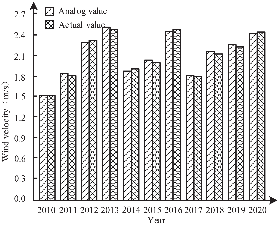
Numerical simulation results of annual average wind speed variation.

Analysis of Figure 4 shows that this method can effectively simulate the average annual wind speed of wind farms, and close to actual wind speed. The results show that the numerical simulation accuracy of the method is 2.5, which can provide accurate numerical simulation for the subsequent evaluation of wind energy resources of wind farms. As can be seen from Figure 4, there is no regular pattern of wind speed change between 2010 and 2020.

Analysis of wind speed and wind power density

The wind tower of the wind farm is analyzed by numerical simulation. Figure 5a represents the hourly wind direction at altitudes of 10, 30, and 50 m. Figure 5b represents the monthly distribution of annual wind speed and wind power density.

Figure 5.

Represents the monthly distribution of annual wind speed and wind power density: (a) monthly variation of wind speed. and (b) monthly distribution of wind power density.

Analysis of Figure 5 shows that the higher the tower height, the greater the corresponding wind speed, the greater the wind power density. The wind speed and wind power density at three kinds of heights are about the same. This wind farm represents the months with high wind speed and power density in the year from May to July and from October to November. The average annual wind speed is about 5.96, 6.7, and 7.0 m/s. The annual mean wind power density is about 288, 326, and 373 W/m².

Taking 50 M height as an example, the daily distribution of wind speed and wind power density on behalf of the wind farm is analyzed by this method. The analysis results are shown in Figure 6.

Figure 6.

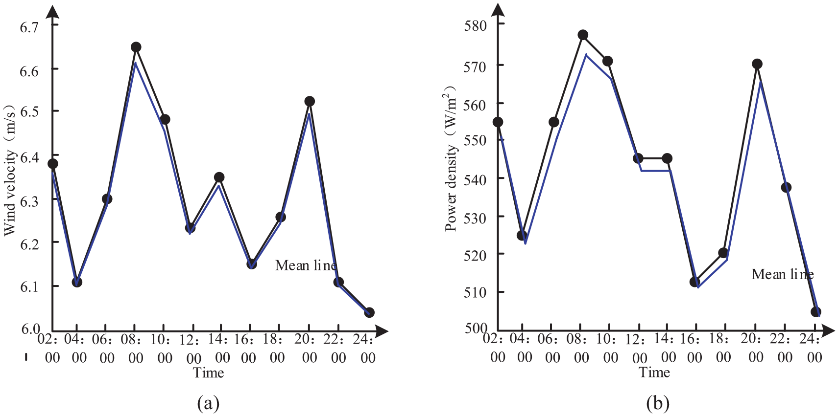
Represents the daily distribution of monthly wind speed and wind power density: (a) daily variation of wind speed. and (b) daily distribution of wind power density.

From the analysis of Figure 6, the change trend of monthly wind speed of wind farm is close to that of solar energy density. The lowest time of day for wind speed and wind power density is 24:00. The maximum time of wind speed and power density is 08:00.

Comprehensive analysis of Figure 5 and Table 1 shows that the wind power density at the height of 10, 30, and 50 m is in the range of wind power grade 3. At the same time, the corresponding wind speed at three altitudes is very close to the reference wind speed, which indicates that the wind power density of the wind farm is at the level of 3. It has good application effect and development potential in wind power application.

Analysis of wind speed and wind direction characteristics

The present method is used to analyze the wind direction and wind energy distribution of the 50 m wind measuring tower. The analysis results are shown in Figures 7 and 8.

Figure 7.

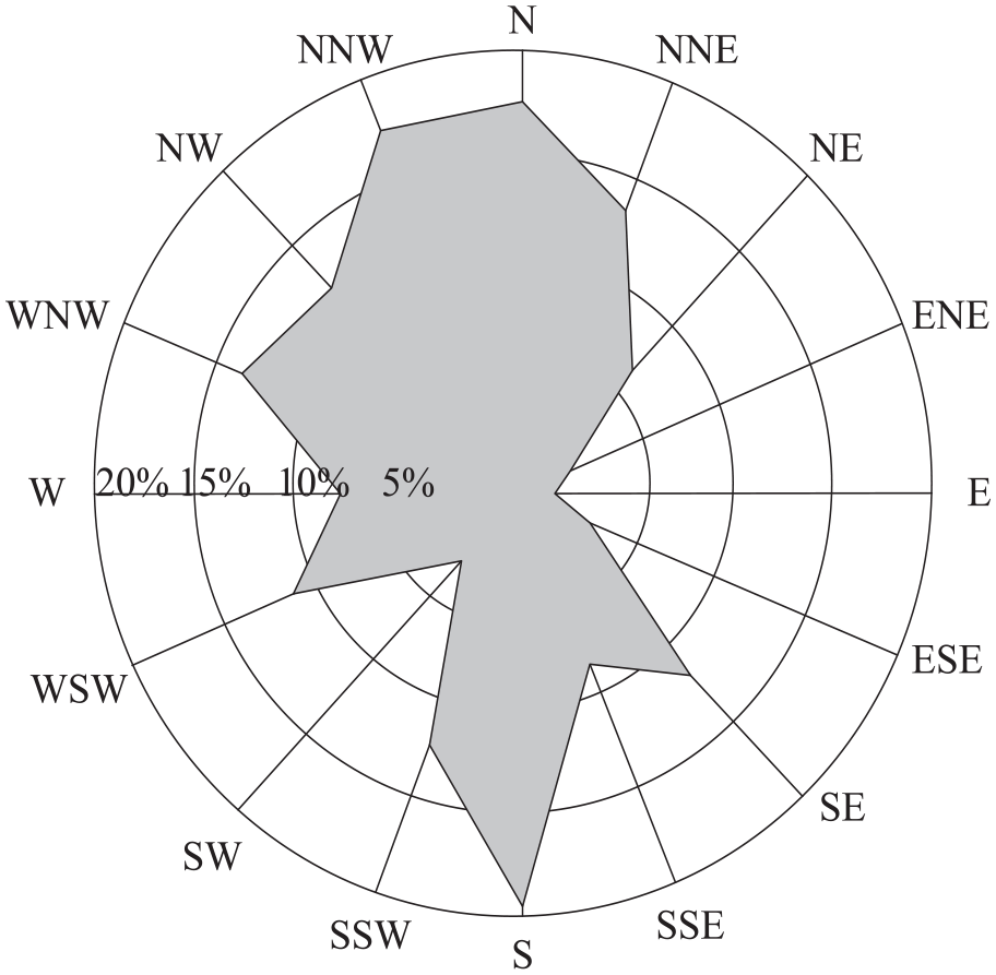
Wind direction analysis results.

Figure 8.

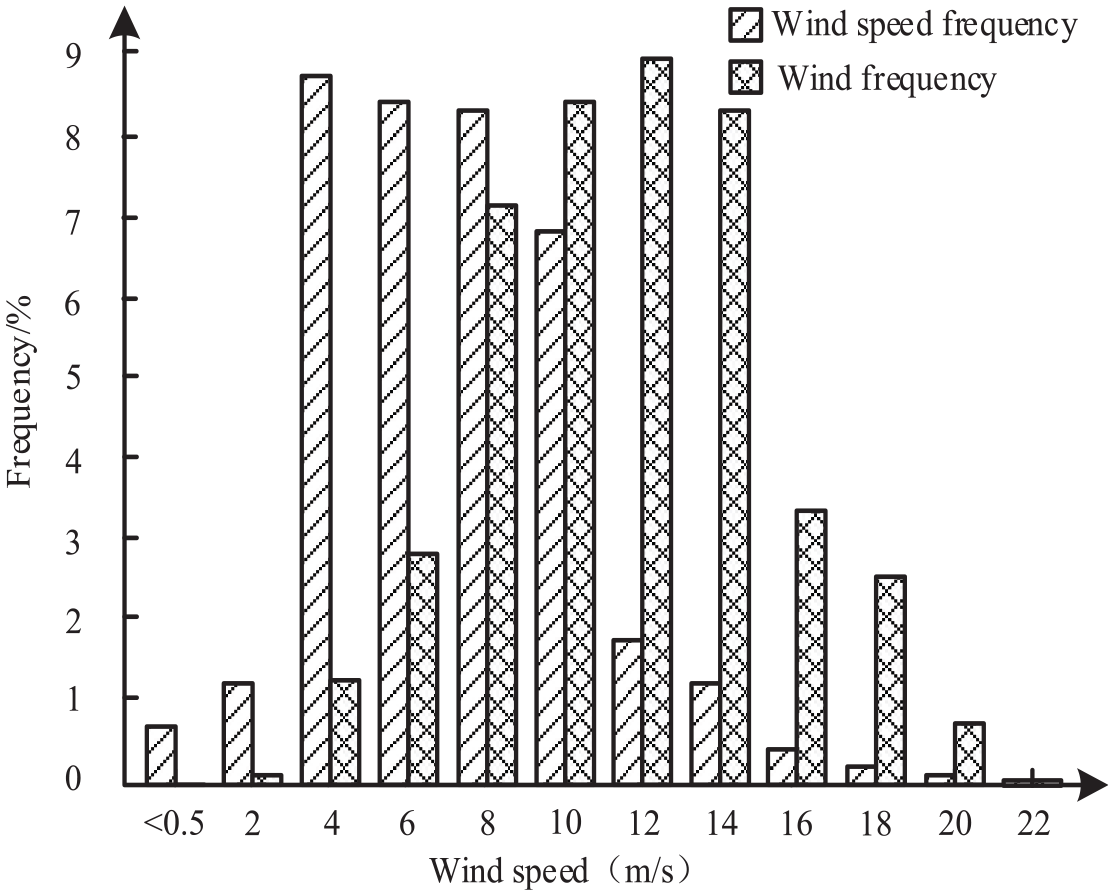
Wind energy distribution.

Analysis of Figure 7 shows that the highest wind frequency of the wind farm at an altitude of 50 m is the south wind (S). This was followed by North West Wind (NNW) and North Wind (N).

Analysis of Figure 8 shows that the wind frequency of the wind farm is basically between 4 and 10 m/s, in the year when the wind speed is relatively high. The wind energy is between 8 m and 14 m/s, and the rest of the wind energy frequencies are relatively small.

The main wind energy is S and the secondary wind energy is NNW and N. The wind energy distribution in the range of the wind farm is dense, which is favorable for the installation of wind turbines and can reduce the loss of wind turbine electricity. The wind speed frequency of the wind farm is basically between 4 m and 10 m/s, and there is no destructive wind speed, which can generate electricity throughout the year.

Turbulence intensity analysis

The intensity of turbulence is the fatigue load that the fan can bear, and the value less than 0.11 can ensure the safe operation of the fan. The turbulence intensity in the 10 m/s wind speed range from 10 to 50 m is analyzed by the present method. The results are shown in Figure 9.

Figure 9.

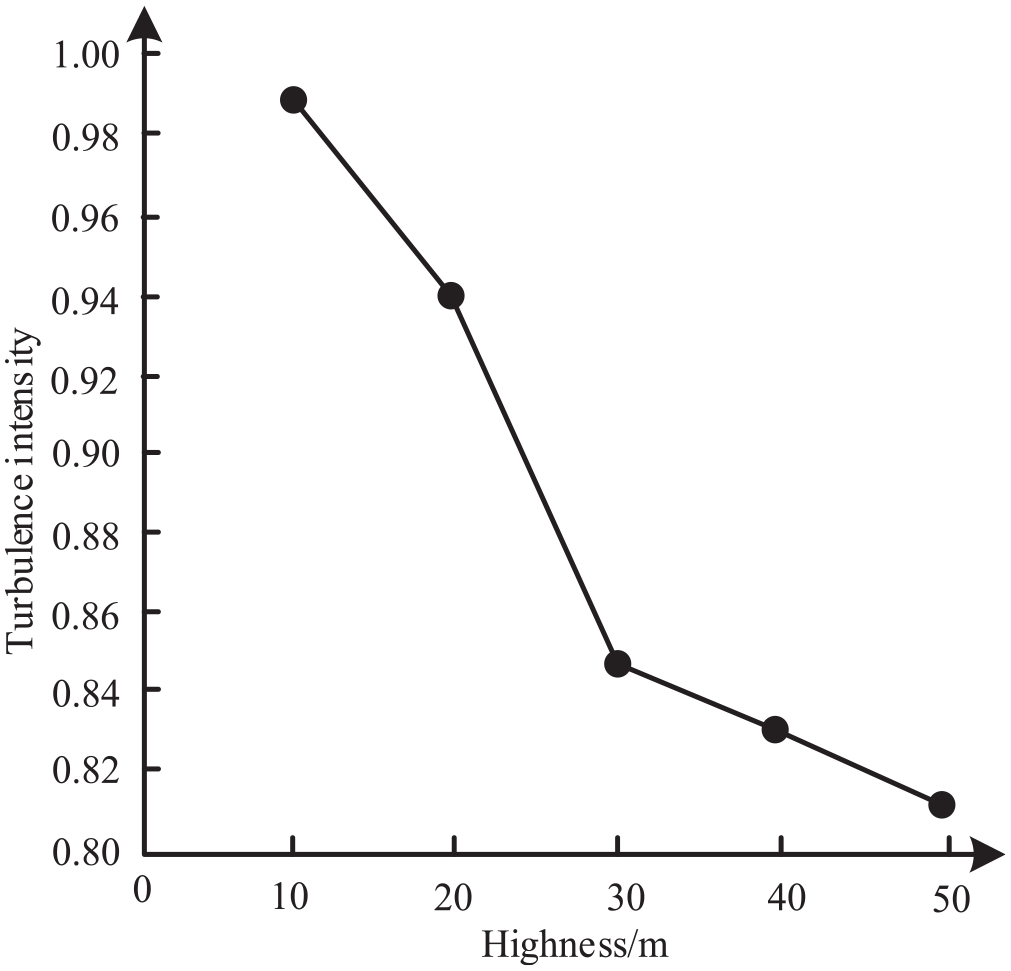
Turbulence intensity analysis results.

Analysis of Figure 9 shows that the turbulence intensity decreases with the increase of height, and the highest turbulence intensity is less than 0.10, which is below the minimum standard. This indicates that the turbulence intensity of the wind farm is not large and the service life of the fan can be effectively prolonged.

Electricity generation assessment

The theoretical power generation simulated by the method in this paper is compared with the theoretical power generation simulated by the method in literature (Ye et al., 2019), and the reliability of this method is verified. The comparison results are shown in Table 2.

Table 2.

Theoretical power generation evaluation results.

Wind velocity (m/s)	Analog frequency/%	Generator power/kW	Methods in this paper power generation/kWh	Measured frequency/%	Generator power/kW	Literature (Ye et al., 2019) Method power generation/kWh
2	1.32	15	28,853.21	1.29	15	28,642.19
4	8.87	27	31,175.43	8.82	27	31,054.32
6	8.53	136	162,982.6	8.55	136	163,893.71
8	8.46	315	335,469.38	8.42	315	334,258.27
10	6.91	565	462,443.83	6.93	565	463,454.94
12	1.99	769	257,118.19	1.96	769	245,007.08
14	1.37	847	146,593.27	1.38	847	146,694.38
16	0.56	859	61,352.75	0.55	859	61,141.86
18	0.33	860	25,682.90	0.33	860	25,582.90
20	0.18	860	12,279.00	0.18	860	12,179.00
22	0.0	860	5967.90	0	860	5867.90

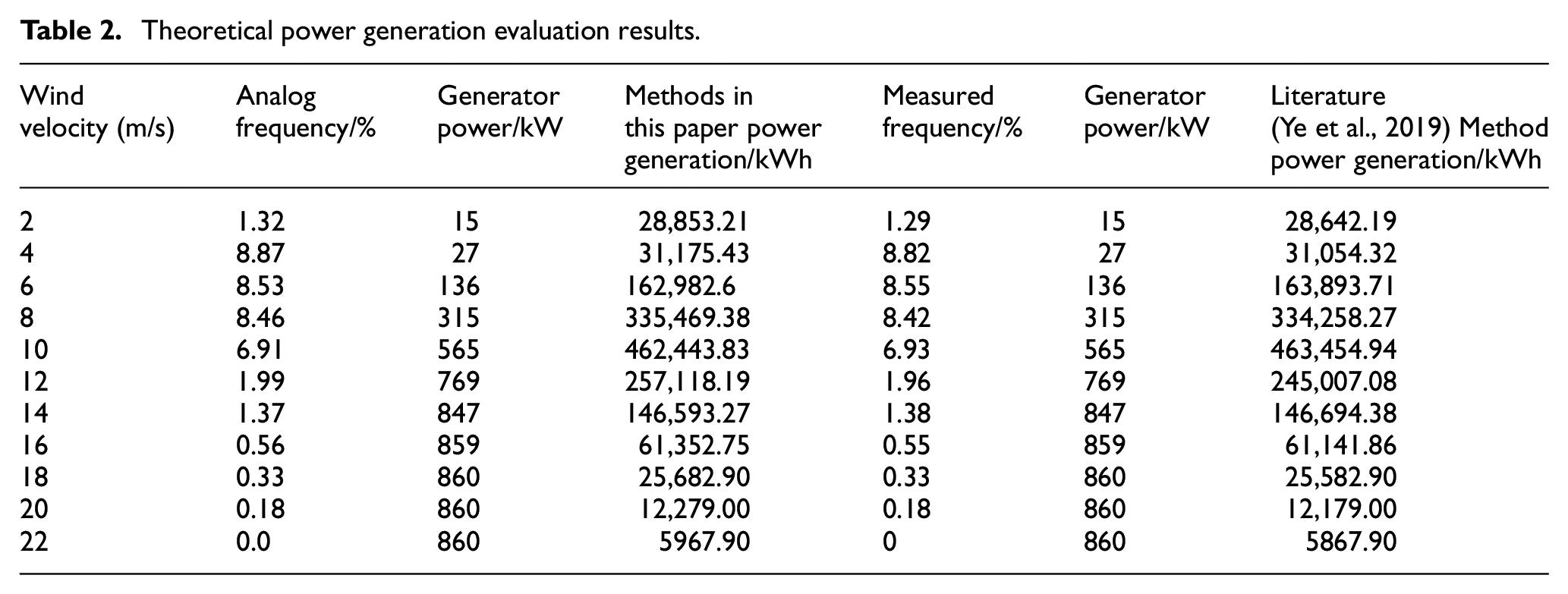
Analysis Table 2 shows that the difference between the simulated wind frequency and the measured wind frequency is small, and the maximum error is only 0.05 kW. The difference between theoretical generation and actual generation is also small. The theoretical power generation is 1,529,918.46 kWh, and the actual theoretical power generation is 1,530,586.55 kWh. The error between theoretical and practical generation is only 0.04%. Compared with the theoretical power generation simulated by the method in Ye et al. (2019), the theoretical power generation simulated by the method in this paper is closer to the actual theoretical power generation. The experimental results show that this method can accurately evaluate the wind energy resources of power plants.

Conclusion

Using the method of mesoscale and microscale nesting to help the wind power projects without wind measurement data, the high resolution wind resource evaluation method based on mesoscale initiation model and CFD technology is studied. The mesoscale WRF numerical model is used to solve the regional data of wind farms and obtain the mesoscale meteorological analysis data. According to the solution results of the mesoscale atmospheric model, the wind speed profile is established, the boundary conditions and initial conditions are extracted, and the CFD micro scale model is input to obtain the wind speed and wind speed frequency at the height of the fan impeller. The reliability of the method is proved by analyzing and comparing the wind resource of the simulated point with the actual data of the wind tower. The method of this paper provides a reference for the development of wind power projects in the future. It is of great significance to objectively judge the development value of wind farms.

Footnotes

Declaration of conflicting interests

The author(s) declared no potential conflicts of interest with respect to the research, authorship, and/or publication of this article.

Funding

The author(s) disclosed receipt of the following financial support for the research, authorship, and/or publication of this article: The study was supported by Key Project of Natural Science Foundation of Ningxia Province, China “Research on precision improvement of quality and efficiency of existing wind farms in Ningxia based on wake effect and non-uniform underlying surface model of wind farm groups (Grant No. 2022AAC02078)” and Ningxia Excellent Talents Programme.

ORCID iD

Junpeng Ma

References

Ding

Song

Sun

, et al. (2019) Scenario generation and evaluation method of multiple wind farms output considering spatial-temporal correlation. Electric Power Automation Equipment 39(10): 39–47.

Han

Zhao

Tong

, et al. (2020) Review and outlook of wind resource assessment methods for wind site located at complex terrain. Thermal Power Generation 49(11): 139–146.

Huang

Sun

Wang

, et al. (2020) Multi-scale simulation of typhoon wind fields by coupling of weather research and forecasting model and large-eddy simulation. Journal of Building Structures 41(2): 63–70.

Jia

Wang

Zhao

, et al. (2019) Numerical analysis of a wind farm unit layout experience based on CFD methods. Renewable Energy Resources 37(5): 762–768.

(2020a) A new index to evaluate offshore wind energy resources. Electric Power Construction 41(5): 108–115.

Liu

Tao

Duan

, et al. (2019) Marine wind farm simulation on group islands based on CFD and linear model. Yangtze River 50(S1): 309–311+349.

Gong

Shi

, et al. (2020b) Prediction and evaluation of wind energy resource in inner Mongolia based on regional climate models. Power System Technology 44(11): 4318–4327.

Wang

Liu

(2020) A wind resource assessment method based on atmospheric stability. Renewable Energy Resources 38(1): 47–52.

Wang

, et al. (2019a) A hindcast dataset on domestic wind energy resource in fine resolution via observation-nudging climate four-dimension data assimilation method. Power System Technology 43(11): 3859–3866.

10.

Wang

Xue

Wang

, et al. (2019b) Probabilistic assessment of multi-state output of wind farms considering the effects of multi-parameters. Advances of Power System & Hydroelectric Engineering 35(2): 69–77.

11.

Yao

Liu

Bai

, et al. (2019) Study of multi-index comprehensive evaluation method for wind farm power prediction level. Acta Energiae Solaris Sinica 40(2): 333–340.

12.

Chen

Jin

, et al. (2019) Measure-correlate-predict assessment method of wind energy resource considering wind power density and wind direction. Automation of Electric Power Systems 43(3): 24–32.

13.

(2020) Flow Field Action and aerodynamic loads distribution for large-scale wind turbine under typhoon based on nesting of WRF and CFD. Acta Energiae Solaris Sinica 41(12): 260–269.

14.

Liu

Xiong

(2019) Application Study of weather research and forecasting (WRF) model in mountainous wind farm with high altitude. Water Power 45(1): 103–106.

15.

Zhang

Cheng

(2020) Numerical simulation of wind field in complex terrain based on CFD downscaling. Plateau Meteorology 39(1): 172–184.