A wind speed interval prediction method for reducing noise uncertainty

Abstract

Due to the noise uncertainty, the conventional point prediction model is difficult to describe the actual characteristics of wind speed and lacks a description of the wind speed fluctuation range. In this paper, the kernel density estimation according to its error value is given, and then its fluctuation range is found to combine the prediction results of the test set to get its prediction range. Firstly, the singular spectrum analysis (SSA) is introduced to conduct the noise reduction, and variational modal decomposition (VMD) is performed to handle the sequences, then an improved slime mold algorithm (SMA) is proposed to optimize the VMD, and the stochastic configuration networks (SCNs) is applied to perform the prediction. Finally, the interval prediction results are calculated by fusing the point prediction error and kernel density estimation. The experimental results demonstrate that the proposed method can effectively reduce the noise interference in the wind speed prediction.

Keywords

Wind speed prediction singular spectrum analysis slime mold algorithm Stochastic configuration networks Noise reduction Variational modal decomposition

Introduction

Research background

Wind energy is a new type of energy with sustainability, which is conducive to the development of a low-carbon economy, and has attracted much attention worldwide in recent years with its great potential. The accurate wind speed prediction is beneficial to the large-scale application of wind resources to power systems (Cui et al., 2020). However, wind power generation depends to a large extent on the variation of wind speed, which is difficult to be used effectively due to its short duration, poor sustainability, and lack of stability, and also makes it more difficult to integrate wind power into the grid (Memarzadeh and Keynia, 2020). Short-term wind speed prediction is the key to alleviating this problem; therefore, improving the accuracy of wind speed prediction is beneficial for wind power system scheduling and is important for the application of wind energy (Li et al., 2018).

Machine learning is a popular field of artificial intelligence research, and models such as neural network (BP) (Emeksiz and Tan, 2022), support vector machine (SVM) (Yousuf et al., 2022), and random forest (RF) (Han et al., 2018) can enhance the extraction of nonlinear features of wind speed series with their powerful nonlinear fitting ability, and compared with the above two methods, artificial intelligence methods can effectively improve the prediction accuracy of short-term wind speed. The combination of prediction models and other algorithms has become the mainstream direction in the field of wind speed prediction research. However, the actual wind speed detection devices are affected by the environment, and the collected data are often mixed with a large amount of noise, which seriously interferes with the prediction accuracy of wind speed. In this paper, a wind speed prediction method to reduce noise uncertainty is developed.

Related works

Data preprocessing methods are becoming increasingly popular in models for predicting wind speeds. The main purpose of data preprocessing is to decompose the wind speed data to reduce the effect of nonlinear effects. Zheng et al. (2021) achieved the decomposition of wind speed signal by the VMD method, which further extracted the time-frequency information to achieve wind speed prediction. Wang et al. (2021) proposed a two-stage data preprocessing method by VMD and Sim Geometric Mode Decomposition (SGMD), and the proposed method is experimentally demonstrated to be suitable for nonlinear wind speed analysis. In addition, signal decomposition methods have also been applied to noise reduction. Liang et al. (2022) decomposed the signal by the VMD method and extracted feature vectors based on IMF signals, and finally, it was experimentally demonstrated that the VMD method not only effectively reduces noise interference but also effectively differentiates time-frequency information.

Nowadays, swarm intelligence optimization algorithms have been studied more deeply, and more and more emerging algorithms have been proposed: sparrow search algorithm (SSA) (Xue and Shen, 2020), arithmetic optimization algorithm (AOA) (Agushaka and Ezugwu, 2021), slime mold algorithm (SMA) (Li et al., 2020), fruit fly optimization algorithm (FOA) (Pan, 2012) and its combination with honey badger algorithm (Li et al., 2024) etc. Based on the continuous development of swarm intelligence optimization algorithms, research on optimized prediction models has received extensive attention. Li et al. (2022b) applied the improved gray wolf optimization algorithm (IGWO) to optimize the parameters of the LSTM model and verified that the proposed hybrid prediction model has the good predictive capability. Han et al. (2022) performed an optimized convolutional neural network (CNN) and bidirectional long and short-term memory network (Bi-LSTM) by grid search (GS) method to complete the prediction. Li et al. (2022a) decomposed the wind speed by VMD and used the particle swarm optimization (PSO) method for each modal component to the Bi-LSTM prediction model to the optimization, proving that the PSO-VMD-Bi-LSTM model is robust to the uncertainty prediction. Wang et al. (2022) decomposed the wind speed series by CEEMDAN, followed by RLMD for the quadratic decomposition of the unsteady series, and constructed the improved whale optimization algorithm (IWOA) optimized LSTM prediction model for each subsequence. Zhang et al. (2022a) decomposed the wind speed time series into multiple intrinsic modal functions (IMFs) by VMD, and used IWOA to optimize the QRGRU model.

However, some machine learning methods in wind speed prediction still have shortcomings. Li and Han (2018) proposed that SVM has problems with poor generalization performance and serious overfitting; BP neural network, as one of the traditional neural networks, has the defects of complex network structure, a large number of hidden layers, long training time, poor generalization ability; Deep learning models CNN and LSTM have high prediction accuracy, but their operation time complexity is too high. Therefore, these prediction models are not the optimal choice for us. Wang and Li (2017) proposed a stochastic configured network in 2017, which gradually increases the hidden layer nodes through the supervision mechanism to ensure the general approximation ability. As a kind of random weight vector network, it has the advantages of efficient operation and strong generalization ability. Therefore, compared with the above models, SCNs are more suitable for wind speed prediction.

Our works

To address the problem that wind speed data containing uncertainty noise can affect the prediction accuracy, this paper proposes an interval prediction method. Firstly, the SSA combined with the improved SMA is used to optimize the VMD to decompose the wind speed sequence into some subsequences, then the SCNs is used to predict each subsequences, and the prediction results are aggregated, and finally, the prediction interval is constructed by the point prediction error and kernel density distribution fitting strategies. The main contributions of this paper are as follows:

(1) An interval prediction method based on point prediction error and kernel density estimation is constructed to reduce the influence of noise uncertainty and improve the prediction accuracy.

(2) An improved slime mold algorithm with multi-strategy fusion (TASMA) is proposed, which has a faster convergence speed and a higher optimization-seeking accuracy.

(3) A data decomposition method based on SSA combined with optimal VMD is designed, to solve the problem that the parameters of VMD are difficult to be determined accurately.

The rest of the framework of this study is organized as follows. Section 2 details the problem and solution proposed in this paper, and presents the wind speed data hybrid prediction model. Sections 3-5 introduce the model principles, SMA fundamentals, improvement mechanisms, and interval prediction principles. Section 6 provides a discussion related to the experimental prediction of the data for the one seasons. Finally, Section 7 concludes the paper.

Propose solutions

Problem statement

In practical application, the wind turbine signal contains mechanical noise, aerodynamic noise caused by weather, sensor transmission interference and other influences. Wind speed noise is generally a kind of data with low amplitude and more intense vibration, which will make the original data bias, increase the complexity of the sequence. Wind speed noise will disrupt the hidden information of the entire data set, and it is difficult to estimate. Its data has unknown, complex and other characteristics, which will increase the difficulty of the later wind speed prediction.

Solutions

Wind speed is affected by the noise disturbance, and the conventional point-based prediction models lack a description of the range of future wind speed fluctuations. Wind speed interval prediction can give confidence intervals, thus reducing the uncertainty of such disturbances. In this paper, we will estimate the kernel density of the training set error, set the confidence interval, calculate the upper and lower bounds of the speed interval, and finally obtain the interval range of wind speed prediction. The predicted model components are combined and superimposed to find their training errors, and the confidence intervals are set according to the kernel density estimation to find their wind speed interval ranges. Finally, the resulting interval is used to describe the wind speed affected by the noise, minimizing the effect of its randomness and uncertainty.

Methodology

The methods involved in this study, such as SSA, VMD, and SCNs, are briefly described below.

SSA

A finite-length one-dimensional time series $[x_{1}, x_{2}, . . ., x_{N}]$ is given, where $N$ is length of the series. Choose a suitable window length $L$ (generally taken as $L < N / 2$ ) to lag-arrange the original time series to obtain the trajectory matrix, and let $K = N - L + 1$ to construct a trajectory matrix of order $L \times K$ , as shown in equation (1).

X = [\begin{matrix} x_{1} & x_{2} & \dots & x_{K} \\ x_{2} & x_{3} & \dots & x_{K + 1} \\ ⋮ & ⋮ & ⋱ & ⋮ \\ x_{L} & x_{L + 1} & \dots & x_{N} \end{matrix}]

(1)

The covariance matrix of the trajectory matrix is firstly calculated according to equation (2).

S = X X^{T}

(2)

Find the matrix $X$ eigenvalues $λ_{1} > λ_{2} > . . . > λ_{L} \geq 0$ (singular spectrum) and the corresponding eigenvectors $U = [U_{1}, U_{2}, . . ., U_{L}]$ , and have:

X = \sum_{m = 1}^{L} \sqrt{λ_{m}} U_{m} V_{m}^{T}, V_{m} = \frac{X^{T} U_{m}}{\sqrt{λ_{m}}}, m = 1, 2, \dots, L

(3)

where $λ_{i}$ corresponds to the feature vector $U_{i}$ .

Divid the set of subscripts {1,2,…, $m$ } into $M$ mutually disjoint subsets $I_{1}, I_{2}, . . ., I_{M}$ , such that $I = {i_{1}, i_{2}, . . ., i_{p}}$ , and it has

X = X_{I 1} + X_{I 2} + \dots + X_{IM}

(4)

The grouping matrix $X$ is defined by

X = {\begin{matrix} \frac{1}{k} \sum_{m = 1}^{k} y_{m},_{k - m + 1}, 1 \leq k < L \\ \frac{1}{L} \sum_{m = 1}^{L} y_{m},_{k - m + 1}, L \leq k < K \\ \frac{1}{T - k + 1} \sum_{m = k - K + 1}^{T - k + 1} y_{m},_{k - m + 1}, K \leq k < T \end{matrix}

(5)

VMD

VMD defines the eigenmode function (IMF) as an amplitude-modulated frequency modulated signal $u_{k} (t)$ with the following expression:

u_{k} (t) = A_{k} (t) c o s (ϕ_{k} (t))

(6)

where $A_{k} (t)$ is the instantaneous amplitude of $u_{k} (t)$ . The constrained model of VMD is formulated as follows:

{\begin{matrix} min_{{u_{k}}, {ω_{k}}} \sum_{k = 1}^{K} ‖ \partial_{t} {[δ (t) + \frac{j}{π t} * u_{k} (t)] e^{- j ω_{k} t}} ‖_{2}^{2} \\ s . t . \sum_{k = 1}^{K} u_{k} = f (t) \end{matrix}

(7)

where $K$ denotes the number of modes to be decomposed; $u_{k}$ , $ω_{k}$ denote the modal components and the center frequency; $\partial_{t}$ denotes the gradient operation; * denotes the convolution operation; and $f (t)$ denotes the original signal.

The Lagrange multiplicative operator $λ$ is introduced to solve equation (7) to obtain equation (8).

\begin{matrix} L ({u_{k} (t)}, {ω_{k} (t)}, λ) = α \sum_{k = 1}^{K} ‖ \partial_{t} {[(δ (t) + \frac{j}{π t}) \times u_{k} (t)] e^{- j ω_{k} t}} ‖_{2}^{2} \\ + ‖ f (t) - \sum_{k = 1}^{K} u_{k} (t) ‖_{2}^{2} + 〈 λ (t), f (t) - \sum_{k = 1}^{K} u_{k} (t) 〉 \end{matrix}

(8)

After the iteration, the expressions of ${\hat{u}}_{k}^{n + 1} (ω)$ , $ω_{k}^{n + 1}$ , and ${\overset{\land}{λ}}^{n + 1} (ω)$ respectively are:

\frac{{\overset{\land}{u}}_{k}^{n + 1} (ω) = \overset{\land}{f} (ω) - \sum_{i < k} {\overset{\land}{u}}_{i}^{n + 1} (ω) + \sum_{i > k} {\overset{\land}{u}}_{i}^{n} (ω) + {\overset{\land}{λ}}^{n} (ω) / 2}{1 + 2 α {(ω - ω_{k}^{n})}^{2}}

(9)

ω_{k}^{n + 1} = \frac{\int_{0}^{+ \infty} ω {| {\overset{\land}{u}}_{k} (ω) |}^{2} d ω}{\int_{0}^{+ \infty} {| {\overset{\land}{u}}_{k} (ω) |}^{2} d ω}

(10)

{\hat{λ}}_{k}^{n + 1} (ω) = {\hat{λ}}_{k}^{n} (ω) + τ (\hat{f} (ω) - \sum_{k = 1}^{K} {\hat{u}}_{k}^{n + 1} (ω))

(11)

where $\hat{f} (ω)$ , ${\hat{u}}_{k} (ω)$ and $\hat{λ} (ω)$ are the Fourier transforms of $f (t)$ , $u_{k} (t)$ , $λ (t)$ . Set the algorithm termination condition as:

\sum_{k = 1}^{K} \frac{‖ {\hat{u}}_{k}^{n + 1} - {\hat{u}}_{k}^{n} ‖_{2}^{2}}{‖ {\hat{u}}_{k}^{n} ‖_{2}^{2}} < ε

(12)

where $ε$ is the allowable accuracy, $ε > 0$ .

Stochastic configuration networks (SCNs)

SCNs proposed by Wang and Li (2017), are incremental stochastic learning neural networks of the RVFLN, which solves its problem of inappropriate settings for random parameters. The structure of the SCNs is shown in Figure 1.

Figure 1.

The flow chart of SCNs.

Given a training set dataset $X = {x_{1}, x_{2}, \dots, x_{k}}$ , its corresponding output $Y = {y_{1}, y_{2}, \dots, y_{k}}$ . Assuming that a single hidden layer feedforward neural network with an $L - 1$ number of hidden nodes has been built, the output of this network can be expressed as:

f_{L - 1} = \sum_{j = 1}^{L - 1} β_{j} g_{j} (w_{j}^{T} X + b_{j}), f_{0} = 0

(13)

where $L = 1, 2, . . .$ denotes the number of hidden nodes, $ω_{j}$ and $β_{j}$ then denote the input weights and bias of the $j th$ hidden node, respectively, $β_{j} = {[β_{j, 1}, β_{j, 2}, \dots, β_{j, m}]}^{T}$ is the output weight of the $j th$ hidden node, and $g_{j}$ is the activation function of the $j th$ hidden node.

Based on the objective function $f$ , the residuals $e_{L - 1}$ of the current network can be obtained:

e_{L - 1} = f - f_{L - 1} = [e_{L - 1, 1}, e_{L - 1, 2}, . . ., e_{L - 1, m}]

(14)

SCNs require random assignment of input weights $ω_{L}$ and biases $b_{L}$ of $L$ hidden nodes under the inequality constraints in

ξ_{L, q} = \frac{{(e_{L - 1, q}^{T} (X) \cdot h_{L} (X))}^{2}}{h_{L}^{T} (X) h_{L} (X)} - (1 - r - μ_{L}) e_{L - 1, q}^{T} (X) e_{L - 1, q} (X) \geq 0

(15)

where $0 < r < 1$ , $0 < μ_{L} < (1 - r)$ and, $lim_{L \to + \infty} μ_{L} = 0$ . $h_{L}^{T} (X)$ denote the output of the $L th$ hidden node.

h_{L} (X) = [g_{L} (w_{L}^{T} x_{1} + b_{L}), . . ., g_{L} (w_{L}^{T} x_{K} + b_{L})]^{T}

(16)

Finally, based on the obtained $ω_{L}$ and the bias $b_{L}$ , the output weights of the whole network are then computed using the least squares method by

β^{*} = {[β_{1}^{*}, β_{2}^{*}, \dots, β_{L}^{*}]}^{T} = H_{L}^{†} Y

(17)

where $H_{L}^{†}$ is the Moore-Penrose inverse of $H_{L} = [h_{1}, h_{2}, \dots, h_{L}]$ .

Improved SMA with multi-strategy fusion

SMA

The position update formula of slime mold in the near food stage is:

X (t + 1) = {\begin{matrix} X_{b} (t) + v_{b} \cdot (W \cdot X_{A} (t) - X_{B} (t)), r < p \\ v_{c} \cdot X (t), r \geq p \end{matrix}

(18)

where $X_{b} (t)$ is the position of the current optimal solution of the population; $v_{b}$ is a random number in the range [ $- a$ , $a$ ], $W$ is the weight coefficient of the slime bacteria; $X_{A} (t)$ and $X_{B} (t)$ are two parent reference positions selected when the population updates its position; $v_{c}$ is a parameter decreasing from 1 to 0; $r$ is a random number in the range [0,1]; $p$ is a parameter of the mathematical model selected when the slime bacteria updates its position. $p$ can be expressed by equation (19).

p = \tanh | S (i) - F_{D} |

(19)

where $S (i)$ is the fitness of slime mold individuals; $F_{D}$ is the best fitness of slime mold in the current iteration.

The value of $a$ is updated by

a = a r c t a n h (- (t / t_{m a x}) + 1)

(20)

where $t$ is the number of current iterations; $t_{m a x}$ denotes the maximum number of iterations.

The weight coefficient $W$ simulates the changes of the oscillators of the body when the slime mold encounters different concentrations of food:

W (SmellIndex (i)) = {\begin{matrix} 1 + rlg ((F_{b} - S (i)) / (F_{b} - F_{w} + 1) \\ 1 - rlg ((F_{b} - S (i)) / (F_{b} - F_{w} + 1), other \end{matrix}

(21)

SmellIndex = s o r t (S)

(22)

where $r$ is a random number of [0,1]; $F_{b}$ and $F_{w}$ are the best and worst fitnesses in the current population iteration; $SmellInde$ denotes the index of individual positions after individual fitness $S$ is sorted in ascending order.

Based on the above theories, the position update formula of slime molds is as follows:

X (t + 1) = {\begin{matrix} r a n d (B_{U} - B_{L}) + B_{L}, r a n d < z \\ X_{b} (t) + v_{b} (W \cdot X_{A} (t) - X_{B} (t)) \\ v_{c} \cdot X (t), r a n d \geq z, r \geq p \end{matrix}, r and \geq z, r < p

(23)

where $B_{U}$ and $B_{L}$ are the upper and lower limits of the search range; $r a n d$ and $r$ are the random numbers in the interval [0,1]; $z$ denotes the ratio parameter of the number of randomly distributed slime mold to the number of overall populations, and $z = 0$ . 03 is chosen in this paper.

Some improvements

Population initialization based on Fuch mapping backward learning

Swarm intelligence algorithms usually use a random strategy of distribution, which can lead to uneven distribution of populations and poor diversity. Fuch mapping can enrich the diversity of populations and enhance the traversal of population initialization. Using the Fuch chaos mapping to generate $X_{t}$ in $M$ -dimensional space as the initial solution, by:

X_{t + 1} = c o s (1 / X_{t}^{2})

(24)

where $X_{t + 1}$ is the chaotic vector at the ( $t + 1$ )th iteration, and the position of each individual is:

X_{i j} = l_{b j} + X_{t + 1} (u_{b j} - l_{b j})

(25)

where $X_{i j}$ denotes the position of the $i th$ slime mold individual in the $j th$ dimension.

Then the reverse learning is used to generate the reverse population by:

T X_{i j} = m (X_{m i n} + X_{m a x}) - X_{i j}

(26)

where $m$ is a random number in the interval [0,1], $X_{m a x}$ and $X_{m i n}$ are the maximum and minimum values of $X_{i j}$ . The population $X$ and the reverse population $TX$ are combined into a new population $X_{new}$ .

Adaptive adjustment of random selection

The original SMA randomly selects two individuals from the population for position update with the parent to generate children, and this random selection increases the global search ability of the algorithm in the early stage but is not conducive to the later convergence of the algorithm. To enhance the convergence of SMA, the selection range of individuals should decrease with the increase in the number of iterations. The selection range parameter $P O$ is described as follows:

P O = c e i l (\frac{P O_{m i n} - P O_{m a x}}{t_{m a x}} \cdot t + P O_{m a x})

(27)

where $P O_{m a x}$ and $P O_{m i n}$ are the maximum and minimum selection range respectively, $P O_{m a x}$ selects $2 / 3 p o p$ population and $P O_{m i n}$ selects $1 / 3 p o p$ population.

Whale spiral mechanism

To better balance the development and search of the SMA, a whale spiral search strategy is introduced by

X_{t + 1} = {\begin{matrix} X_{t}^{b e s t} + e^{l} \cdot c o s (l \cdot 2 π) \cdot (X_{t}^{b e s t} - X_{i}^{t}) \\ l = 1 - 2 (\frac{t}{t_{m a x}}) \end{matrix}

(28)

Depending on the parameter conditions, the modified position update equation is defined by

X_{t + 1} = {\begin{matrix} r a n d \cdot (ub - lb) + lb, r a n d < z \\ X_{b} (t) + v_{b} (W \cdot X_{A} (t) - X_{B} (t)), z \leq r a n d < p & r a n d < 0.9 \\ X_{t}^{b e s t} + e^{l} \cdot c o s (l \cdot 2 π) \cdot (X_{t}^{b e s t} - X_{i}^{t}), z \leq r a n d < p & r a n d \geq 0.9 \\ v_{c} \cdot X (t), z \leq r a n d & p \leq r a n d \end{matrix}

(29)

Expanding global search capability

To enhance the development capability of the underlying artificial swarm, the optimal position guidance strategy is chosen to improve the update mechanism, and there is:

Z_{i, j} = x_{i, j} + r (x_{i, j} - x_{k, j}) + c (p_{g, j} - x_{i, j})

(30)

where $r$ is a random number in [−1,1], $c$ is a random number in [0,1.5], and $p_{g}$ is the global optimal position of the population.

According to equation (30), the late search capability is expanded and the effect of falling into local extreme value points is reduced.

Main steps of improved SMA with multi-strategy fusion (TASMA)

Main steps of TASMA algorithm are shown in the below.

Step 1. Parameter initialization: set the search upper bound $u_{b}$ , lower bound $l_{b}$ , population size $N$ , maximum number of iterations $t_{m a x}$ , and dimension $D$ .

Step 2. Initialize the population: the Fuch mapping reverse learning generates the initial population.

Step 3. Calculate the fitness of each individual of the population and rank them, record the best fitness $F_{B}$ and the worst fitness $F_{W}$ .

Step 4. Select the range of population with better fitness according to equation (27).

Step 5. Update the candidate solution positions according to equation (29).

Step 6. Update the population according to equation (30) and retain the better individuals according to the greedy strategy.

Step 7. Terminate the algorithm if the iteration condition is satisfied, otherwise repeat Steps 3–6.

Step 8. Output the optimal value and the algorithm ends.

The pseudocode of the improved TASMA algorithm is shown in Algorithm1 .

Algorithm 1

TASMA algorithm

Input: Initial population size pop, solution space dimension dim, upper bound

u_{b}

and lower bound

l_{b}

of the solution, the maximum number of iterations

t_{m a x}

.
Output: Global best position

X_{b e s t}

and best fitness value

f_{b e s t}

.
1: Begin procedure
2: Setting related parameters
3: Generate the chaotic initial population
4: New populations were obtained by inverse learning
5: while

t \leq t_{m a x}

do
6: Calculate the slime molds hunger degrees and sorted;
7: Determine the optimal position and optimum fitness;
8: Update

a

by equation (20);
9: Calculate the

W

by equation (21);
10: Update

P O

by equation (27);
11: for each search solution
12: Update

p

v_{b}

v_{c}

l

;
13: Update1 positions by equation (29);
14: Update2 positions by equation (30);
15: end for
16:

t = t + 1

17: end while
18: Display

X_{b e s t}

and

f_{b e s t}

19: End procedure

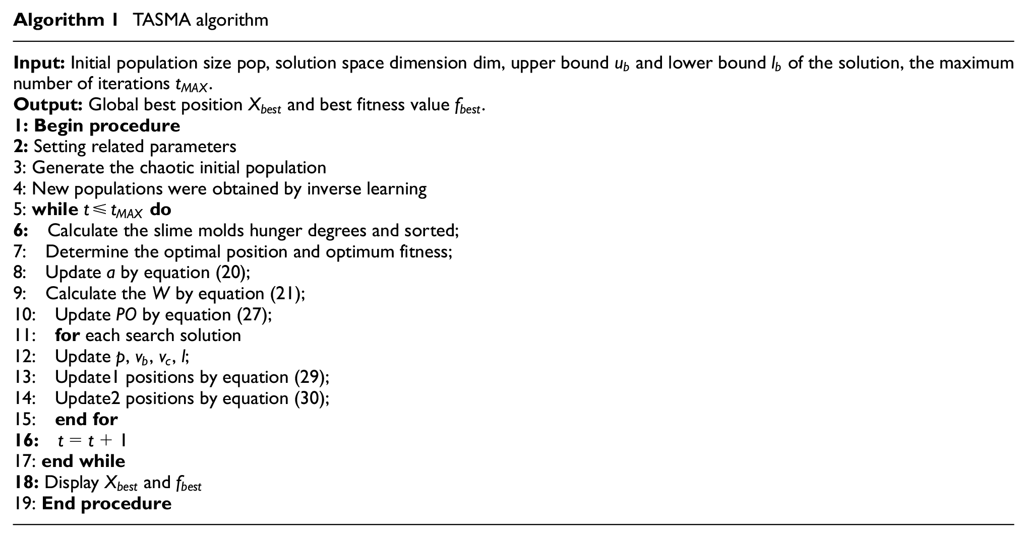
The flow chart of the improved TASMA algorithm is shown in Figure 2.

Figure 2.

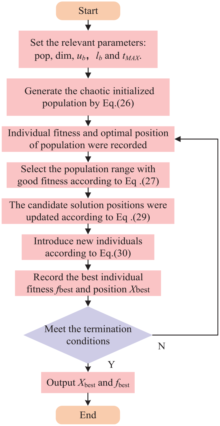
Flow chart of the improved TASMA algorithm.

Interval prediction model

Principle of interval prediction

The traditional point-based prediction models have difficulty in describing the actual characteristics of wind speed and lack the description of the range of future wind speed fluctuations. Wind speed interval prediction can give confidence intervals, which can describe the variation of future wind speed. Parametric estimation requires prior assumptions that the data obey some distribution, whereas nonparametric estimation does not require prior assumptions about the data distribution and can directly fit its distribution based on the data characteristics Zhang et al. (2022b). Although the wind speed prediction error is close to the Gaussian distribution, its wind speed time series is nonlinear in nature, the error of wind speed prediction is not inferred with sufficient a priori knowledge, and the error will also have a certain skewness asymmetry, so the nonparametric kernel density estimation method is used. The interval prediction range can be obtained based on the probability density curve, as follows:

1) Calculate the prediction error of the training set. Find the error between the predicted and measured values of wind speed $e$ :

e = q_{i} - \overset{\land}{q_{i}}

(31)

where $q_{i}$ , $\overset{\land}{q_{i}}$ , are the measured and predicted values of wind speed, respectively.

2) Estimation of the distribution of errors. A nonparametric kernel density estimation is used to obtain the probability density curve of the prediction error:

f (e) = \frac{1}{N h} \sum_{m = 1}^{N} K (\frac{e - e_{i}}{h})

(32)

where $N$ is the total number of samples; $h$ is the width of the window, taken in 1.8–2.0, $e_{i}$ is the $i - th$ error sample, $K (\cdot)$ is the kernel function, and the Gaussian kernel function is taken in this paper.

3) Given the confidence level 1- $α$ , the prediction interval can be expressed as:

[\overset{\land}{q_{i}} + F_{α / 2}, \overset{\land}{q_{i}} - F_{1 - α / 2}]

(33)

where $\overset{\land}{q_{i}}$ is the predicted wind speed, $[F_{α / 2}$ , $F_{1 - α / 2}]$ is the upper and lower bound of the error confidence interval, $\overset{\land}{q_{i}} + F_{α / 2}$ and $\overset{\land}{q_{i}} - F_{1 - α / 2}$ are the upper and lower bound of the predicted interval.

Finally, the closed interval enclosed by its upper and lower boundaries is the prediction result of the model, and it is judged whether the actual value falls in the interval, and if it falls in the interval, the prediction is proved to be valid.

System structure

The structure diagram of the designed system is shown in Figure 3.

Step 1: Obtain wind speed data, and simulate the data set affected by noise.

Step 2: Data pre-processing is performed using SSA to extract different components of the data.

Step 3: The main parameters $α$ and $K$ of VMD are optimized by an improved SMA algorithm, and the decomposed series by the SSA-TASMA-VMD method is used for data prediction.

Step 4: The model components of the signal decomposition are predicted by SCNs, and then the training set errors are obtained.

Step 5: Based on the kernel density estimation error, and the wind speed prediction results of the test set, the wind speed interval is obtained.

Figure 3.

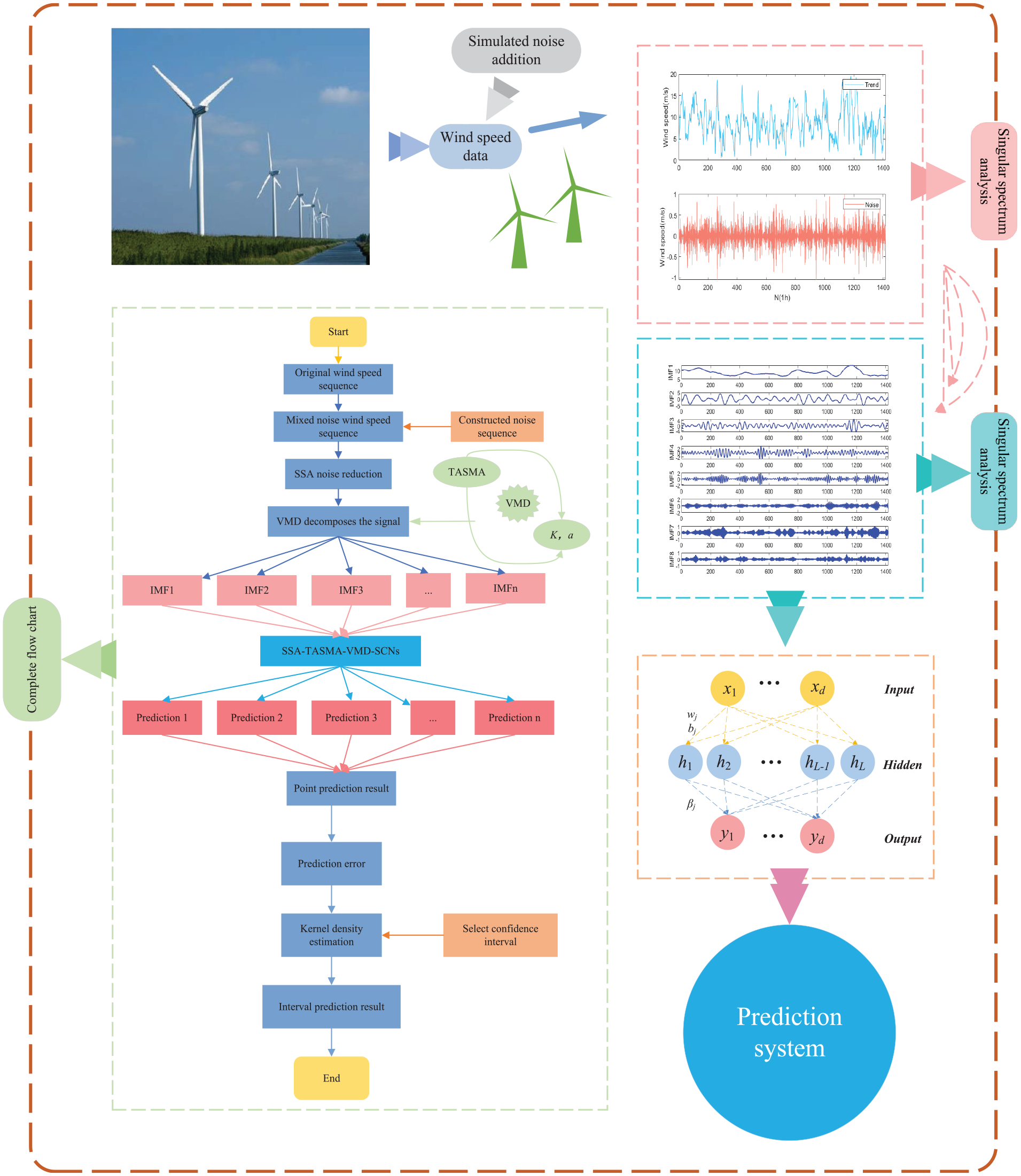
Block diagram of system structure.

Experiments and analysis

In this research paper, the wind speed data from Chicago, USA, 2022 was used, https://www.glerl.noaa.gov/metdata/chi/, in which, 1 hour time interval wind speed series and one seasonal partial data (spring) were used to do the following experiments. The training set and test set are divided according to the ratio of 85%:15%. The wind speed dataset information is shown in Figure 4.

Figure 4.

Infographic of wind speed dataset.

Evaluation metrics

Coverage probability

The prediction interval coverage represents the probability that the true values fall in the prediction interval. The larger the $P I C P$ , the more true values are included in the prediction interval, and the stronger the reliability of the interval.

P I C P = \frac{1}{N} \sum_{i = 1}^{N} ε_{i}

(34)

where $N$ is the number of predicted samples; $ε_{i}$ is variable, if $y_{i}$ falls within the prediction interval, then $ε_{i} = 1$ , otherwise $ε_{i} = 0$ .

Average width of prediction interval

The average width of the prediction interval indicates the width of the interval results. Since a large width due to the simple pursuit of high interval coverage makes the prediction interval lose its meaning, the average width is added as another measure, and its formula is:

P I N A W = \frac{1}{N R} \sum_{i = 1}^{n} (U_{i} - L_{i})

(35)

where $n$ is the number of samples; $R$ is the range of variation of predicted values; $U_{i}$ and $L_{i}$ represent the upper and lower limits.

Predictive interval score

The clarity of the prediction interval is a necessary indicator to assess the merit of the prediction interval Gao et al. (2022).

$v_{t}^{(α)} x (i)$ is defined as the width of PI:

v_{t}^{(α)} x (i) = {\tilde{U}}_{t}^{(α)} x (i) - {\tilde{L}}_{t}^{(α)} x (i)

(36)

The interval fraction of PI denoted by ${IS}_{t}^{(α)} x (i)$ is defined as:

{IS}_{t}^{(α)} x (i) = {\begin{matrix} - 2 α v_{t}^{(α)} x (i) - 4 [{\tilde{L}}_{t}^{(α)} x (i) - T_{i}], if T_{i} < {\tilde{L}}_{t}^{(α)} x (i) \\ - 2 α v_{t}^{(α)} x (i), if T_{i} \in {\tilde{I}}_{t}^{(α)} x (i) \\ - 2 α v_{t}^{(α)} x (i) - 4 [T_{i} - {\tilde{U}}_{t}^{(α)} x (i)], if T_{i} > {\tilde{U}}_{t}^{(α)} x (i) \end{matrix}

(37)

$I_{t}^{(α)} x (i)$ is between $U_{t}^{(α)} x (i)$ and $L_{t}^{(α)} x (i)$ and defines the total score ${IS}_{t}^{(α)}$ for the entire test data set:

{IS}_{t}^{(α)} = \frac{1}{N_{t}} \sum_{i = 1}^{Nt} {IS}_{t}^{(α)} x (i)

(38)

where $α$ is the confidence interval. A smaller absolute score $I S_{t}$ indicates higher clarity and higher interval quality.

Simulation experiments

The parameter settings of the algorithm used in the experiments are shown in Table 1, and for the simulated noise data, the common noise addition coefficients for each season are shown in Table 2, and the proportion of mixed noise addition is shown in Table 3, and it should be noted that the parameters of VMD-SCNs are selected according to the decomposition results (Li et al., 2017).

Table 1.

Model parameter setting.

Model	Parameter settings
TASMA-VMD	$Z = 0.03$ , $k \in [2, 16]$ , $α \in [500, 3000]$ .
SMA-VMD	$Z = 0.03$ , $k \in [2, 16]$ , $α \in [500, 3000]$ .
GRU	hidden codes = 10.
SSA	$L = 288$ , Cumulative contribution rate = 99.5%.

Table 2.

Noise addition scheme.

Model	Noise type	Mean value	Variance	Proportionality coefficient	Serial number
Jan and Feb	Normal	0	0.2	0.1	1
Jan and Feb	Uniform	−0.3	0.5	0.1	2

Table 3.

Mixed noise addition ratio.

Months	Normal noise ratio	Uniform noise ratio	Proportionality coefficient	Serial number
Jan and Feb	0.6	0.4	0.1	3

The noise parameter settings for the uniform and normal distributions are shown in Table 2. For example, in Table 2, the data for January and February are dataset 1, the Mean value of adding Normal noise is 0, the variance is 0.2, the proportion of noise is 0.1, and record its noise data number is serial number 1. The Mean value of the Uniform noise is −0.3, the variance is 0.5, the proportion of the noise is 0.1.

The mixed noise settings are shown in Table 3. For example, in Table 3, the data of January and February are data set 1, and the Uniform and Normal noise in Table 2 are added together. The proportional coefficient of uniform distributed noise is 0.6, the normal distributed noise coefficient is 0.4, and the noise proportional coefficient is 0.1.

After adding the serial number 1 noise in Table 2 to the January–February wind speed data, the signal decomposition and singular spectrum decomposition were performed according to the parameter settings of Table 1, and the decomposition plots are shown in Figure 5.

Figure 5.

Data curve of several key production parameters: (a) EMD, (b) VMD, (c) SMA-VMD, and (d) TASMA-VMD.

Interval prediction results of SCNs, SCNs-Epane (Epanechnikov kernel function), SCNs-Trian (Triangular kernel function), GRU, LSTM, GRNN, EMD-SCNs, VMD-SCNs, VMD-SCNs-res (VMD decomposition with residual sequence), SSA-VMD-SCNs, SSA-SMA-VMD-SCNs, and SSA-TASMA-VMD-SCNs after adding the serial number 1 noise are shown in Figure 6.

Figure 6.

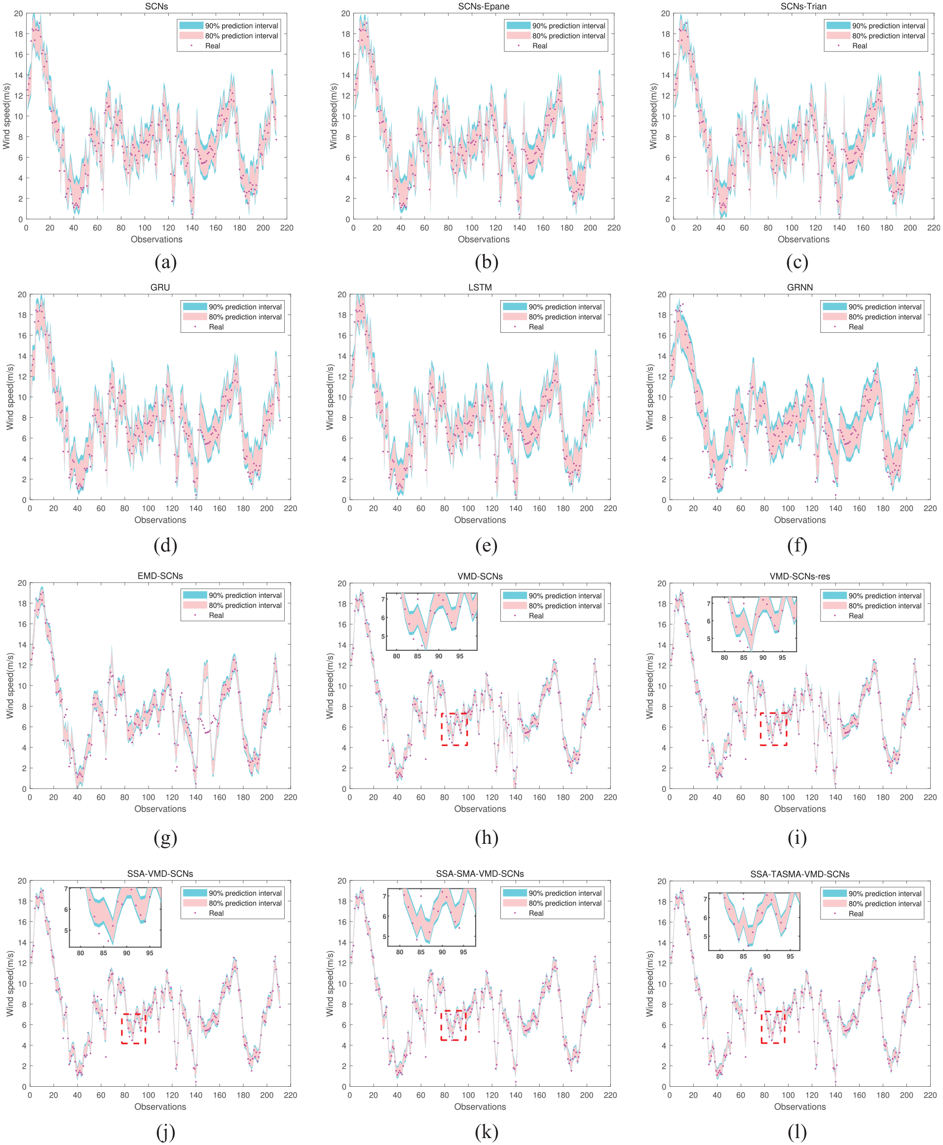
Comparison results of different models after adding serial number 1 noise to dataset 1: (a) SCNs, (b) SCNs-Epane, (c) SCNs-Trian, (d) GRU, (e) LSTM, (f) GRNN, (g) EMD-SCNs, (h) VMD-SCNs, (i) VMD-SCNs-res, (j) SSA-VMD-SCNs, (k) SSA-SMA-VMD-SCNs, and (l) SSA-TASMA-VMD-SCNs.

Through adding serial number 1 noise in Table 2 to the dataset 1, the results of the predictions of the 12 different methods, with 90% and 80% interval coverage and average width of the intervals compared are shown in Figure 7.

Figure 7.

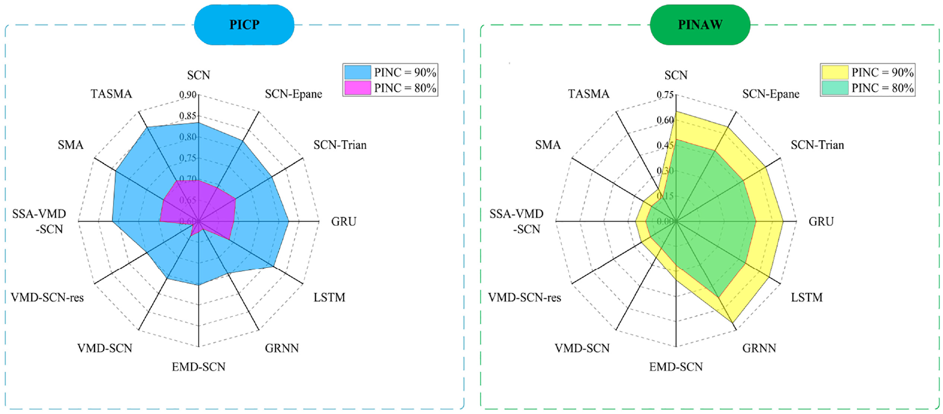
Comparison of the evaluation metrics of different models after adding serial number 1 noise to dataset 1.

In Table 4, the prediction results of wind speed data with serial number 1 noise show that by the comparison of model 1, model 2, and model 3, it can be seen that the Gaussian kernel density estimation predicts the obtained intervals with higher performance than the Epanechnikov kernel function and Triangular kernel function. Comparison of model 1, model 4, model 5 and model 6 shows that the SCNs-based interval prediction performance is better. Comparison of model 7 and model 8 shows that the adding of the residual sequence reduces the performance of interval prediction. The average width of the intervals of the model proposed in this paper is reduced by 66.1% and the fraction of the intervals is improved by 66.5% compared to SCNs at 90% confidence interval, and the average width of the intervals of the model proposed in this paper is reduced by 65.9% and the fraction of the intervals is improved by 66.7% compared to SCNs at 80% confidence interval.

Table 4.

Interval prediction results after adding serial number 1 noise in Table 2.

Noise 1	90% PICP	90% PINAW	90% IS	80% PICP	80% PINAW	80% IS
1.SCNs	0.8341	0.6525	−6.3382	0.6967	0.4858	−4.4841
2.SCNs-Epane	0.8199	0.6455	−6.3557	0.6919	0.4839	−4.5585
3.SCNs-Trian	0.8104	0.6438	−6.3494	0.7062	0.4834	−4.5515
4.GRU	0.8246	0.6674	−6.4705	0.6872	0.4975	−4.5902
5.LSTM	0.8152	0.6679	−6.5485	0.6872	0.4987	−4.7278
6.GRNN	0.7441	0.7037	−7.0835	0.6209	0.5283	−5.236
7.EMD-SCNs	0.7536	0.3528	−3.9557	0.6256	0.2617	−2.9757
8.VMD-SCNs	0.7583	0.2495	−2.4959	0.6398	0.1849	−1.8103
9.VMD-SCNs-res	0.7488	0.2495	−2.5508	0.6161	0.1854	−1.8687
10.SSA-VMD-SCNs	0.8152	0.2536	−2.4546	0.6967	0.1901	−1.7389
11.SSA-SMA-VMD-SCNs	0.8389	0.2356	−2.2673	0.7014	0.1778	−1.6035
12.SSA-TASMA-VMD-SCNs	0.8578	0.2215	−2.1208	0.7109	0.1662	−1.4937

Through adding serial number 2 noise in Table 2 to the dataset 1, the results of the predictions of the 12 different methods, with 90% and 80% interval coverage and average width of the intervals compared are shown in Figure 8.

Figure 8.

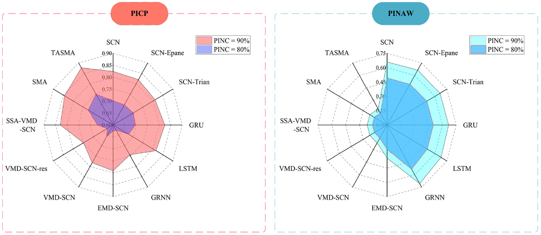
Comparison of the evaluation metrics of different models after adding serial number 2 noise to dataset 1.

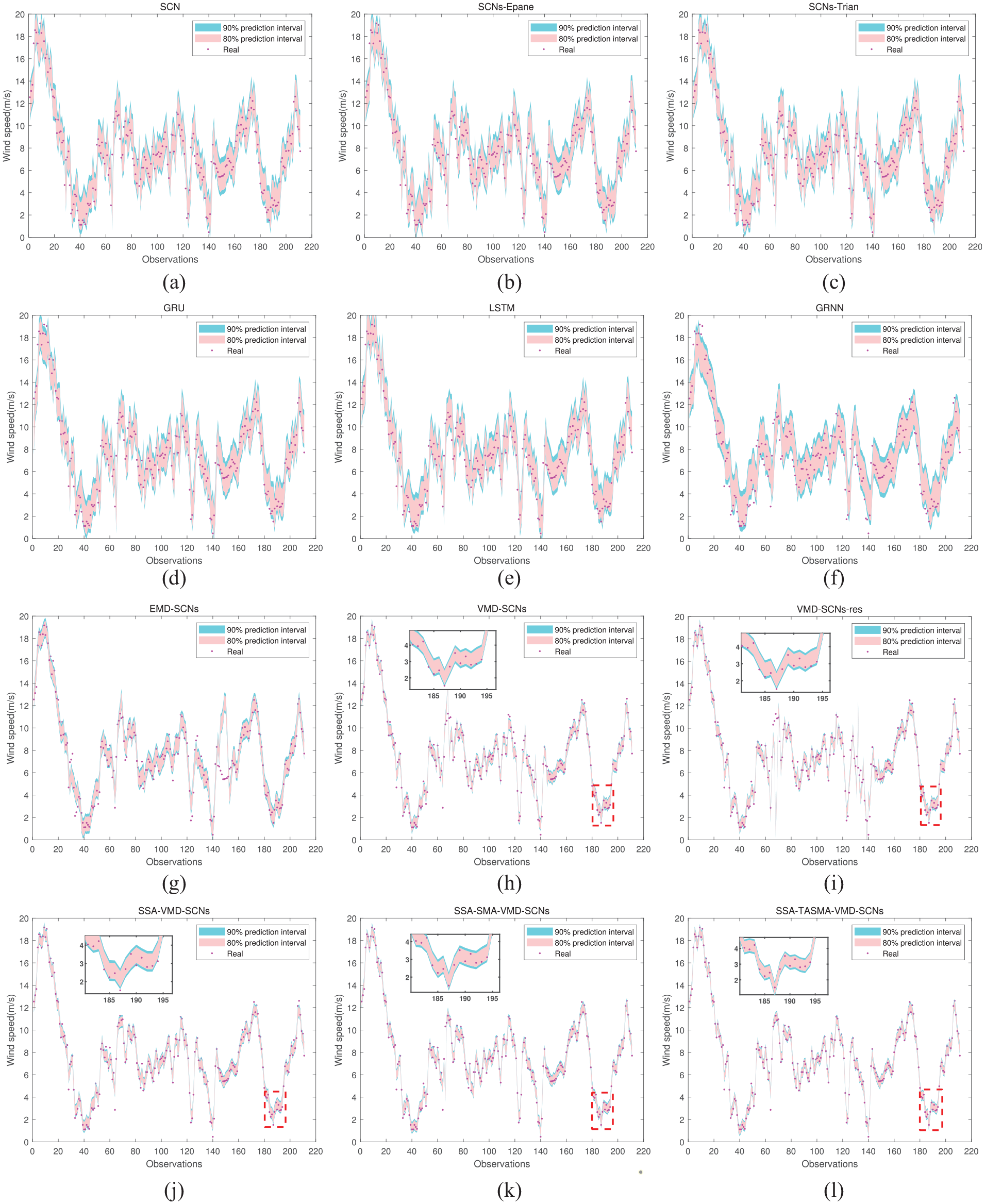
The interval prediction results of different models after adding the serial number 2 noise are shown in Figure 9.

Figure 9.

Comparison results of different models after adding serial number 2 noise to dataset 1: (a) SCNs, (b) SCNs-Epane, (c) SCNs-Trian, (d) GRU, (e) LSTM, (f) GRNN, (g) EMD-SCNs, (h) VMD-SCNs, (i) VMD-SCNs-res, (j) SSA-VMD-SCNs, (k) SSA-SMA-VMD-SCNs, and (l) SSA-TASMA-VMD-SCNs.

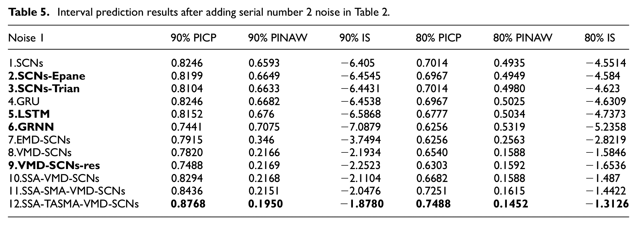
In Table 5, the prediction results of wind speed data with serial number 2 noise show that by the comparison of model 1, model 2, and model 3, it also can be seen that the Gaussian kernel density estimation predicts the obtained intervals with higher performance than other two kernel functions. Comparison of model 1, model 4, model 5, and model 6 shows that the SCNs-based interval prediction performance is also the better. Comparison of model 7 and model 8 also shows that the adding of the residual sequence reduces the performance of interval prediction. The average width of the intervals of the model proposed in this paper is reduced by 70.4% and the fraction of the intervals is improved by 70.7% compared to SCNs at 90% confidence interval, and the average width of the intervals of the model proposed in this paper is reduced by 70.6% and the fraction of the intervals is improved by 71.2% compared to SCNs at 80% confidence interval.

Table 5.

Interval prediction results after adding serial number 2 noise in Table 2.

Noise 1	90% PICP	90% PINAW	90% IS	80% PICP	80% PINAW	80% IS
1.SCNs	0.8246	0.6593	−6.405	0.7014	0.4935	−4.5514
2.SCNs-Epane	0.8199	0.6649	−6.4545	0.6967	0.4949	−4.584
3.SCNs-Trian	0.8104	0.6633	−6.4431	0.7014	0.4980	−4.623
4.GRU	0.8246	0.6682	−6.4538	0.6967	0.5025	−4.6309
5.LSTM	0.8152	0.676	−6.5868	0.6777	0.5034	−4.7373
6.GRNN	0.7441	0.7075	−7.0879	0.6256	0.5319	−5.2358
7.EMD-SCNs	0.7915	0.346	−3.7494	0.6256	0.2563	−2.8219
8.VMD-SCNs	0.7820	0.2166	−2.1934	0.6540	0.1588	−1.5846
9.VMD-SCNs-res	0.7488	0.2169	−2.2523	0.6303	0.1592	−1.6536
10.SSA-VMD-SCNs	0.8294	0.2168	−2.1104	0.6682	0.1588	−1.487
11.SSA-SMA-VMD-SCNs	0.8436	0.2151	−2.0476	0.7251	0.1615	−1.4422
12.SSA-TASMA-VMD-SCNs	0.8768	0.1950	−1.8780	0.7488	0.1452	−1.3126

The interval prediction results of different models after adding the serial number 3 noise are shown in Figure 10.

Figure 10.

Comparison results of different models after adding serial number 3 noise to dataset 1:(a) SCNs, (b) SCNs-Epane, (c) SCNs-Trian, (d) GRU, (e) LSTM, (f) GRNN, (g) EMD-SCNs, (h) VMD-SCNs, (i) VMD-SCNs-res, (j) SSA-VMD-SCNs, (k) SSA-SMA-VMD-SCNs, and (l) SSA-TASMA-VMD-SCNs.

Through adding serial number 3 noise in Table 3 to the dataset 1, the results of the predictions of the 12 different methods, with 90% and 80% interval coverage and average width of the intervals compared are shown in Figure 11.

Figure 11.

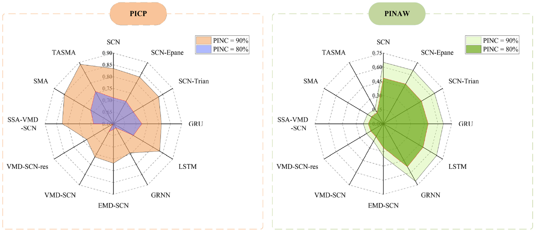
Comparison of the evaluation metrics of different models after adding serial number 3 noise to dataset 1.

In Table 6, the prediction results of wind speed data with serial number 3 noise show that by the comparison of model 1, model 2, and model 3, it also can be seen that the Gaussian kernel density estimation predicts the obtained intervals with higher performance than other two kernel functions. Comparison of model 1, model 4, model 5 and model 6 shows that the SCNs-based interval prediction performance is also the better. Comparison of model 7 and model 8 also shows that the adding of the residual sequence reduces the performance of interval prediction. The average width of the intervals of the model proposed in this paper is reduced by 72.1% and the fraction of the intervals is improved by 72.5% compared to SCNs at 90% confidence interval, and the average width of the intervals of the model proposed in this paper is reduced by 71.8% and the fraction of the intervals is improved by 72.6% compared to SCNs at 80% confidence interval.

Table 6.

Interval prediction results after adding serial number 3 noise in Table 3.

Noise 1	90% PICP	90% PINAW	90% IS	80% PICP	80% PINAW	80% IS
1.SCNs	0.8341	0.6508	−6.3234	0.7109	0.485	−4.4702
2.SCNs-Epane	0.8294	0.6540	−6.3629	0.7109	0.4875	−4.5174
3.SCNs-Trian	0.8294	0.6475	−6.3549	0.7014	0.4825	−4.5061
4.GRU	0.8104	0.6581	−6.3852	0.7251	0.4913	−4.5023
5.LSTM	0.8341	0.6746	−6.5464	0.7014	0.5027	−4.6691
6.GRNN	0.7441	0.7049	−7.0667	0.6209	0.5275	−5.2123
7.EMD-SCNs	0.7678	0.3474	−3.9358	0.6256	0.2554	−2.9681
8.VMD-SCNs	0.7630	0.2149	−2.1955	0.6398	0.1613	−1.6087
9.VMD-SCNs-res	0.7346	0.2138	−2.2868	0.6019	0.1607	−1.7146
10.SSA-VMD-SCNs	0.8246	0.2199	−2.1171	0.6872	0.1664	−1.5197
11.SSA-SMA-VMD-SCNs	0.8483	0.2018	−1.9477	0.7156	0.1506	−1.3744
12.SSA-TASMA-VMD-SCNs	0.8910	0.1818	−1.7368	0.7583	0.1370	−1.2238

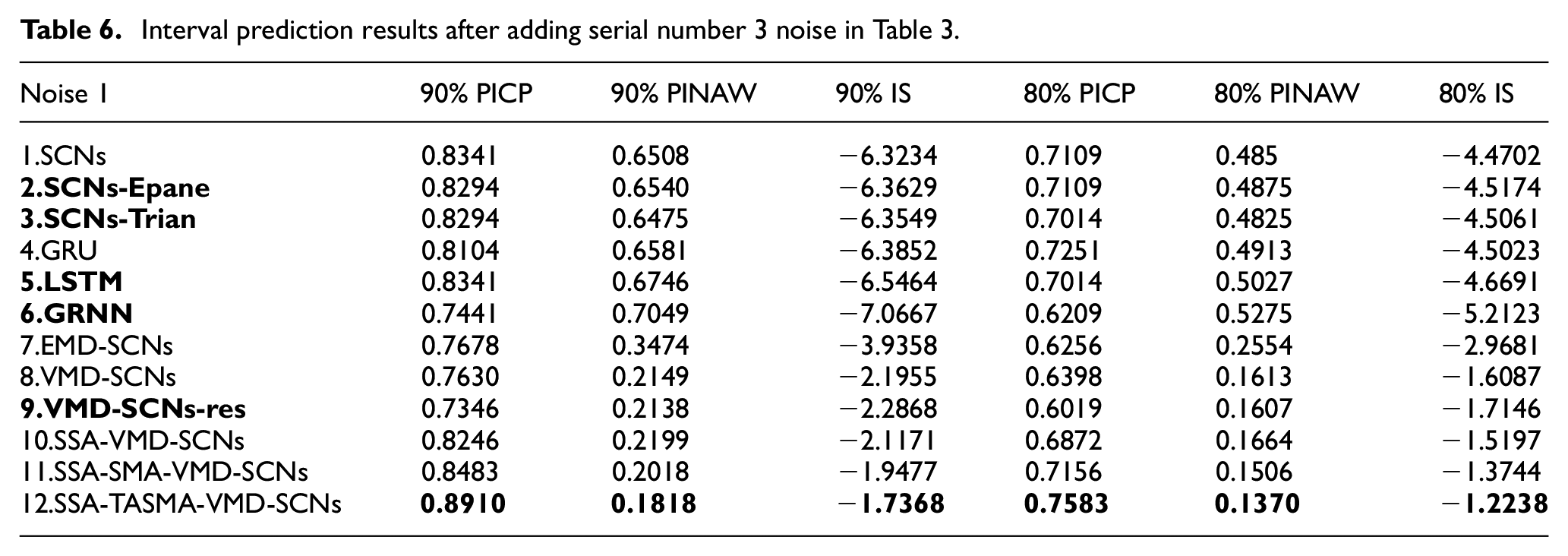
From above, the prediction results of wind speed data containing serial numbers 1–3 noises show that the coverage, mean width, and interval fraction of 90% and 80% confidence intervals of the method proposed in this paper are better than other methods, and the proposed method can reduce the noise uncertainty and achieve effective prediction.

Conclusions

In this paper, we propose a hybrid wind speed prediction system and the hybrid model combines data denoising, signal decomposition optimization, model prediction, and interval conversion to improve the performance of wind speed prediction in a noisy interference environment. The proposed hybrid system achieves good results in short-term wind speed prediction by using the interval prediction method to reduce the interference from noise in wind speed prediction through point prediction error and kernel density estimation fitting strategy. Based on the experimental proof, the hybrid wind speed prediction model after optimizing the parameters can better reduce the wind speed prediction interference by noise.

The complexity of the model in the optimization process will inevitably cause an increase in the prediction time cost, so it is one of our next work plans to further reduce the prediction time while ensuring the prediction accuracy.

Footnotes

Declaration of conflicting interests

The author(s) declared no potential conflicts of interest with respect to the research, authorship, and/or publication of this article.

Funding

The author(s) disclosed receipt of the following financial support for the research, authorship, and/or publication of this article: This work was supported by the LiaoNing Revitalization Talents Prograrn (Grant Number XLYC2007091); this work was also partly supported by the National Natural Science Foundation of China (Grant Number 62203197).

ORCID iD

Ying Han

Data availability

All data included in this study are available upon request by contact with the corresponding author. The used data sets are public domain resources and were obtained from the Chicago, USA, 2022, available at .

References

Agushaka

Ezugwu

(2021) Advanced arithmetic optimization algorithm for solving mechanical engineering design problems. PLoS One 16(8): e0255703.

Cui

Huang

Cui

(2020) A novel compound wind speed forecasting model based on the back propagation neural network optimized by bat algorithm. Environmental Science and Pollution Research 27: 7353–7365.

Emeksiz

Tan

(2022) Multi-step wind speed forecasting and hurst analysis using novel hybrid secondary decomposition approach. Energy 238: 121764.

Gao

Wang

Zhang

, et al. (2022) Ensemble wind speed prediction system based on envelope decomposition method and fuzzy inference evaluation of predictability. Applied Soft Computing 124: 109010.

Han

, et al. (2018) Short-term wind speed forecasting based on signal decomposing algorithm and hybrid linear/nonlinear models. Energies 11(11): 2976.

Han

Shen

, et al. (2022) A short-term wind speed prediction method utilizing novel hybrid deep learning algorithms to correct numerical weather forecasting. Applied Energy312: 118777.

Liang

Zhao

Shi

(2022) A novel combined model based on VMD and IMODA for wind speed forecasting. Journal of Intelligent & Fuzzy Systems 42(4): 2845–2861.

Song

Wang

, et al. (2022a) A novel offshore wind farm typhoon wind speed prediction model based on PSO–bi-LSTM improved by VMD. Energy 251: 123848.

Han

(2018) Modelling for motor load torque with dynamic load changes of beam pumping units based on a serial hybrid model. Transactions of the Institute of Measurement and Control 40(3): 903–917.

10.

Yan

Han

(2024) Multi-mechanism swarm optimization for multi-uav task assignment and path planning in transmission line inspection under multi-wind field. Applied Soft Computing 150: 111033. DOI: 10.1016/j.asoc.2023.111033

11.

Chen

Wang

, et al. (2020) Slime mould algorithm: A new method for stochastic optimization. Future Generation Computer Systems 111: 300–323.

12.

Chen

, et al. (2017) A novel feature extraction method for ship-radiated noise based on variational mode decomposition and multi-scale permutation entropy. Entropy 19(7): 342.

13.

Peng

Zhang

, et al. (2022b) Multi-step ahead wind speed forecasting approach coupling maximal overlap discrete wavelet transform, improved grey wolf optimization algorithm and long short-term memory. Renewable Energy 196: 1115–1126.

14.

Liu

(2018) Multi-step wind speed forecasting using EWT decomposition, LSTM principal computing, RELM subordinate computing and IEWT reconstruction. Energy Conversion and Management 167: 203–219.

15.

Memarzadeh

Keynia

(2020) A new short-term wind speed forecasting method based on fine-tuned LSTM neural network and optimal input sets. Energy Conversion and Management 213: 112824.

16.

Pan

(2012) A new fruit fly optimization algorithm: taking the financial distress model as an example. Knowledge-Based Systems 26: 69–74.

17.

Wang

(2017) Stochastic configuration networks: Fundamentals and algorithms. IEEE Transactions on Cybernetics 47(10): 3466–3479.

18.

Wang

Xiong

Chen

, et al. (2022) Multi-step ahead wind speed prediction based on a two-step decomposition technique and prediction model parameter optimization. Energy Reports 8: 6086–6100.

19.

Wang

, et al. (2021) Design of a combined system based on two-stage data preprocessing and multi-objective optimization for wind speed prediction. Energy 231: 121125.

20.

Xue

Shen

(2020) A novel swarm intelligence optimization approach: Sparrow search algorithm. Systems Science & Control Engineering 8(1): 22–34.

21.

Yousuf

Al-Bahadly

Avci

(2022) Statistical wind speed forecasting models for small sample datasets: Problems, improvements, and prospects. Energy Conversion and Management 261: 115658.

22.

Zhang

Hua

, et al. (2022a) Evolutionary quantile regression gated recurrent unit network based on variational mode decomposition, improved whale optimization algorithm for probabilistic short-term wind speed prediction. Renewable Energy 197: 668–682.

23.

Zhang

Liu

, et al. (2022b) Wind power interval prediction based on hybrid semi-cloud model and nonparametric kernel density estimation. Energy Reports 8: 1068–1078.

24.

Zheng

Dong

Liu

, et al. (2021) Multistep wind speed forecasting based on a hybrid model of VMD and nonlinear autoregressive neural network. Journal of Mathematics 2021: 1–9.