Individual investor portfolio performance in retirement savings accounts

Abstract

We analyse the investment performance of a large sample of individuals investing in discretionary superannuation products offered by a large Australian financial institution. We do not find gender differences as has previously been reported but we do find evidence of a negative relationship between investor age and performance. Those residing in wealthier postcodes perform better. In terms of investment characteristics, wholesale investors perform better whereas those who are the most active perform worse.

Keywords

Household portfolios investment choice portfolio performance retirement savings superannuation

1. Introduction

Successfully managing an investment portfolio, measured as persistently meeting or exceeding a suitable risk-adjusted benchmark, is a difficult task. From an efficient market perspective we should not expect consistent outperformance relative to such benchmarks and available evidence highlights the difficulty for professional investors to do so (Busse et al., 2010; Malkiel, 2005). In short, the results are ‘disheartening’ for investors (Fama and French, 2010: 1916). Australian evidence is similar, with a number of studies unable to identify persistent superior risk-adjusted returns and/or market timing ability (Bird et al., 1983; Gallagher, 2001; Gallagher and Jarnecic, 2002; Holmes and Faff, 2004, 2008; Jones et al., 2008; Sinclair, 1990) though some contrary, ‘heartening’, results are noted (In et al., 2013; Pinnuck, 2004) as well as Gallagher (2003) who also finds some ability in predicting risk-adjusted returns.

Individual investors are increasingly provided with similar opportunities to make significant investment decisions. Retirement savings, via superannuation, is a case in point. Government policy continues to transfer responsibility for making investment decisions to individuals in the absence of evidence suggesting individual investment competence to do so. In contrast to the large literature that has examined professional fund management investment behaviour and performance, comparatively few studies have investigated individual investor behaviour. Where they have (Calvet et al., 2006; Grinblatt and Keloharju, 2001a; Guiso and Jappelli, 2006) a consistent finding is, as Barber et al. (2009) succinctly summarise: ‘Individuals lose, institutions win’ (p.1). In terms of aggregate fund flows, findings had previously been more promising suggesting a ‘smart-money’ effect among individual investors (Gruber, 1996) such that money flows to those funds that subsequently outperform. Gharghori et al. (2007) confirm the finding for Australia funds, countering the suggestion that the result was a result of the momentum effect (Sapp and Tiwari, 2004).

More recently, the performance of superannuation funds has been considered in terms of the impact of illiquid investments (Cummings and Ellis, 2011) and fund size (Cummings, 2012). The current paper is, however, focused on the performance of individuals within superannuation funds. In this area Gharghori et al. (2008) is the closest to our focus as they investigate aggregate individual investor flows, finding no ‘smart money’ effect within Australian superannuation funds. No available evidence documents how the members of Australian superannuation funds perform individually, that is, in their individual account history. Given that superannuation assets now exceed AUD$1.5 trillion (Australian Prudential Regulation Authority, 2013) and are a key component of the government retirement incomes policy, this is a notable absence in the literature.

A feature of the Australian superannuation system, in common with international trends, has been the decline of the defined benefit (DB) fund in favour of defined contribution (DC) funds (Gerrans and Clark, 2013). The key distinguishing feature of DB and DC funds is that the responsibility for investment performance is borne by the individual in DC funds and by the sponsor, primarily, in DB funds. A frequent lament however, as voiced by the Chairman of the Australian Securities and Investments Commission, is that individuals’ ‘level of engagement with superannuation is quite low’ (Medcraft, 2012). More alarming is the claim that ‘many consumers do not have the interest, information or expertise required to make informed choices’ (Commonwealth of Australia, 2010: 5). Thus, this paper addresses the central research question of how well do individuals in personal superannuation products perform with their investment selection.

The underlying transaction level data is supplied by a large Australian financial institution for its flagship superannuation product which offers an investment menu containing over 100 options across all asset classes. While the institution does provide financial advice to its clients as required, our data refers only to those investors who are not advised. This allows us to focus on individual investment decisions, as distinct from the decisions made by individuals under advice. With the monthly return data covering the period from January 2002 to January 2012, we are able to estimate risk-adjusted performance measures at the individual investor level. This provides insight into the performance of individual investment portfolios.

We find performance is better for those we would generally characterise, a priori, as sophisticated. That is, wholesale clients who live in higher income postcodes. High levels of switching are found to be detrimental to performance as is age, though the latter is not robust across periods. In contrast to prevailing literature, we do not find evidence that male investors underperform female investors given the risk-adjusted returns used in our study. While we find no consistent result for rebalancing activity, the results in our analysis suggest this is an area worthy of future research. A review of relevant literature is presented in the following section. Data are described more fully in Section 3. A discussion of the analysis is provided in Section 4 and conclusions and further research opportunities are discussed in Section 5.

2. Literature review

The recent research into individual investor decision making relies either on experiments or on analysis of historical records of individual investment transactions. Experimental studies create a setting within which the trading behaviour of a sample of investors, ranging from naïve to experienced investors, can be observed (Anderson et al., 2007; Haigh and List, 2005; Kluger and Wyatt, 2004; Lo et al., 2005; Porter and Smith, 2003). These studies can provide considerable insight into investor behaviour in a very controlled setting but there are limitations to this approach. For example, it is often difficult to attract appropriate participants and it can also be quite difficult to create an experimental setting that encourages realistic investment decisions.

Analysis of historical records of investor trading also provides insight into individual investor decision making, though this cannot be controlled in the same way that experiments can be controlled. In this case it is necessary to impute investment decisions from actual investor trades. There is considerable literature in this area ranging from descriptions of investor characteristics and choices (Clark-Murphy and Soutar, 2004; Clark-Murphy et al., 2002; Lewellen et al., 1977) to evidence of excessive trading (Barber and Odean, 2000b, 2001), individual trading behaviour (Barber et al., 2003; Barber and Odean, 2000a), performance extrapolation (Benartzi, 2001), loss aversion (Bernatzi and Thaler, 1995; Grinblatt and Keloharju, 2001b; Odean, 1998), online trading (Barber and Odean, 2002) and analysis of what attracts investors to particular investments (Barber and Odean, 2008). This literature is firmly anchored to what has happened in the market through the use of individual investor transaction data and so there is no question about incentives or appropriateness of the setting as this data describes actual trading behaviour. The problem with much of this research is the reliance on cross-sectional data. Yet, there are some examples where individual transactions are tracked over time (Barber and Odean, 2000b) and the current study adds to this literature.

Claims of a lack of engagement in superannuation are supported by a range of studies reporting low levels of investment activity in retirement savings plans (Choi et al., 2002; Clark-Murphy et al., 2009; Hedesstrom et al., 2004; Mitchell et al., 2006). Yamaguchi et al. (2006) identify literature suggesting value decreasing outcomes due to profound inertia at one extreme, that is individuals don’t trade even where net marginal benefits are available, to excessive trading at the other extreme due to overconfidence in the value of information signals. Utilising a comprehensive dataset of US 401(k) plans, Tang et al. (2009) contrast the generally efficient investment menus chosen by plan sponsors with the large number of plan participants who choose inefficient portfolios. Yamaguchi et al. (2006) use a more granular approach examining participant trading activity and find the higher raw returns for traders is largely attributed to the increased risk of traders. Those who rebalance either passively (that is selecting a blended option such as balanced) or actively (by trading to return to an initial allocation choice) outperform on a risk-adjusted basis. In contrast, those who actively trade reduce risk-adjusted performance significantly.

In relation to superannuation, Drew (2006) highlights the difficulty of successful investment timing and possible negative impact of switching using simulated data, though with the exception of Gerrans et al. (2008), individual superannuation investment choice and performance remain largely unexplored in the literature. Of particular note is the considerable flexibility that superannuation products offer individual investors in terms of the ability to change the weighting allocated to broad asset classes within their superannuation portfolio (equity, cash, fixed interest and property). This paper provides insight into the impact of individual investor decision making on the performance of their personal superannuation portfolio over the period from January 2002 to January 2012.

Given the nature of the data, we are able to explore issues including the impact of the global financial crisis (GFC) on the status quo effect or excessive trading with the onset of the GFC. The GFC is a period of considerable volatility, providing a natural experiment for analysis of how individual investors react to a dramatic fall in the value of the equity market and the rather unusual market behaviour that took place following the crisis. In this analysis we are specifically concerned with the impact of biases and behaviour on individual investment decisions.

The question concerning how investors behave in a financial crisis is a vexed one, though research into the behaviour of loss-averse investors does provide some insight (Kahneman and Tversky, 1984; Kahneman et al., 1991). If our investors are loss averse and their reference point does not change with the onset of the crisis, then they will tend to do nothing. In effect, the loss-averse investor exhibits risk-seeking behaviour, holding onto the loss-making investment as its value continues to plunge. This tendency to avoid realising losses, and so maintain the status quo, has been noted in the literature (Fry et al., 2007; Odean, 1998) though few studies have focused on trading behaviour over a period quite so dramatic as the GFC with the exception of Gerrans (2012) who documents spikes in trading activity in the worst months of the GFC but low levels of trading activity overall.

This study also provides insight into the impact of mental accounting on investment decisions (Thaler, 1999). Where an investment is viewed as a form of saving, it is possible that the status quo effect may be further reinforced as individuals segregate and protect their retirement fund-based investments. Some of the investors in the sample have automatic payments made into their accounts and we posit that mental accounting may further enhance the status quo effect for this type of investor.

Crises could result in excessive trading by investors who change their investment preferences from equity to cash or fixed interest securities. These investors may dramatically increase their sales of equity and purchases of alternative securities around a crisis like the recent GFC (Barber and Odean, 2000b). If they react too slowly then this strategy could realise losses and lock the investors into low yielding asset classes. The low interest rates evident since the GFC began would be particularly damaging for investors who sold at the bottom of the equity market in 2008.

3. Data

Our data is supplied by a large Australian financial institution. We focus on two products from the institution in this analysis: personal superannuation and wholesale personal superannuation. These products are subject to similar institutional constraints and clients in both face the same investment menu and choice options. Wholesale personal superannuation accounts tend to be larger which suggests that those investing in this product will be wealthier and perhaps better informed in terms of their knowledge of superannuation and investment decision making more generally. Investors have an investment menu which extends to over 100 options covering the full range of asset classes. This includes specific asset class options (e.g. Australian Equity) and blended options (e.g. Balanced which includes cash, equity and property). Investors can make a change to their investment allocation at no administrative cost but incur the bid/ask spread for options transacted.

Investors in the products do not receive financial planning advice from the institution’s financial advice arm. Neither have they invested in the product via an advised channel. While this does not preclude investors having received advice elsewhere it does ensure the individuals in our sample have the opportunity to freely choose among the range of products offered by the institution. This aspect of the data avoids the in-house financial adviser effect noted in the literature (Hackethal et al., 2012) though it should also be noted that investors may choose to ignore financial advice even when they seek it out (Bhattacharya et al., 2012). We argue that the focus of our research is on individual investor behaviour where the individual freely chooses their investment and so our experimental design specifically excludes those that are advised. The performance of advised clients will reflect the investment policy of the adviser and in this case there is just one adviser, the financial institution, that is primarily responsible for providing advice. It is likely that the addition of advised clients will add little variability to the data set as the advised client portfolios will tend to follow the financial institution recommendation. Thus, while adding advised investors might increase the sample size it is unlikely that it will increase the cross-sectional variation in the individual performance that we focus on in this study.

The data set consists of two files. The first file type contains a snapshot of investors at the end of January 2012. This file includes data on some 15,468 non-advised individual investors, including gender, age (years) and location (postcode). The second file contains all transactions recorded for each investor from which 800,556 monthly individual investor return observations are calculated. This trading data spans the period January 1998 to January 2012, though we focus on the period from January 2002 as there are few observations available prior to January 2002 (1307 monthly observations in total). A further 200 monthly observations are dropped due to missing unit price information, leaving 799,048 monthly return observations available for analysis. Customer activity increases rapidly over the study period, with around 868 monthly return observations recorded for 2002, increasing to around 100,000 in 2007, and then to 167,000 in 2011. To gain further insight into the impact on individual investor performance of the GFC, separate analysis is conducted for two sub-periods. We term the first sub-period the pre-GFC period and this spans the period from January 2002 to September 2007. The second sub-period is called the post-GFC period and it spans the period from August 2009 through to January 2012. These break points fit the broad movements in the Australian stock exchange reasonably well as can be seen from Figure 1, while avoiding the turbulence of the GFC period itself. The first sub-period, from January 2002 to September 2007, covers a period of strong growth in the equity market while the second sub-period, August 2009 through to January 2012, covers a period of little growth with considerable volatility.

Figure 1.

S&P/ASX 300 total return index.

Descriptive statistics are reported in Table 1 for monthly return data over the full study period. This data is used in calculation of portfolio performance. There are 799,048 investor-month returns available for analysis over the 121 month sample period. The mean individual investor month return (MTHRET) and standard deviation are 0.00092 (or 1.11% per annum) and 0.03708 (or 12.84% per annum) respectively with mean risk-free rate adjusted individual investor return (MTHRET_RF) and standard deviation of −0.00342 (or −4.03% per annum) and 0.03740 (or 12.96% per annum) respectively.¹ We also collect risk factors over the 121 month sample period from Datastream for use in calculation of alphas. The Australian share market risk premium (RMAUS_RF) is calculated by deducting the yield on a 30-day bank accepted bill (BAB30), expressed as a rate per month, from the total return on the S&P/ASX 300 index for the month (SPASX300R). The mean return on the equity market risk premium is 0.00096 (1.16% per annum) with standard deviation of 0.03965 (13.73% per annum) over the 10-year study period.

Table 1.

Descriptive statistics: Variables used in alpha estimation.

Number of observations (N), mean, standard deviation (SD), minimum (Min.), 5 percentile (P5), median (P50), 95 percentile (P95) and the maximum (Max.) are reported for each of the variables used in calculation of alphas for the individual investors included in our sample. MTHRET is the total monthly return calculated for each individual for each month that they hold an investment in the products offered by the financial institution. SPASX300R is the total month return for the S&P/ASX 300 share price index. BAB30 is the yield on a 30 day bank accepted bill, which is used as a proxy for the risk-free rate. MTHRET_RF is the risk-free rate adjusted individual portfolio monthly return. RMAUS_RF is the risk-free rate adjusted monthly return on the S&P/ASX 300 share price index. UBSBOND is the total monthly return on the UBS Australian composite bond index which includes all maturities. SPASXPROP is the total return on the S&P Australian property index. MSCIWLDR is the total return on the MSCI world index. MSCISML is the difference in the return earned on the MSCI Australian Small stock index and the MSCI Australian large stock index. MSCIHML is the difference in the return earned on the MSCI Australian value stock index and the MSCI Australian growth stock index. All returns are expressed as a decimal rate of return per month.

Variable	N	Mean	SD	Min.	p5	p50	p95	Max.
MTHRET	799048	0.00092	0.03708	−0.53026	−0.06371	0.00321	0.05296	0.38516
MTHRET_RF	799048	−0.00342	0.03740	−0.53635	−0.06906	−0.00099	0.04924	0.38256
SPASX300R	121	0.00534	0.03942	−0.13792	−0.06481	0.01447	0.05548	0.07761
RMAUS_RF	121	0.00096	0.03965	−0.14402	−0.06884	0.01060	0.05248	0.07414
BAB30	121	0.00438	0.00089	0.00259	0.00268	0.00422	0.00609	0.00637
UBSBOND	121	0.00518	0.00802	−0.01237	−0.00750	0.00495	0.01772	0.02890
SPASXPROP	121	0.00007	0.05642	−0.34082	−0.09212	0.00867	0.05934	0.15185
MSCIWLDR	121	0.00358	0.04940	−0.20753	−0.08810	0.00982	0.07677	0.10725
MSCISML	121	0.00230	0.03199	−0.17797	−0.05147	0.00498	0.04783	0.06734
MSCIHML	121	−0.00227	0.03231	−0.09351	−0.04585	−0.00126	0.04198	0.14984

The size premium (MSCISML), used in the Fama and French (1993) three-factor model, is defined as the total return on the MSCI Australia small firm index less the total return on the Morgan Stanley Composite Index (MSCI) Australia large firm index. The value premium (MSCIHML), also used in the Fama and French three-factor model, is defined as the total return on the MSCI Australia value firm index less the total return on the MSCI Australia growth firm index. We use commercially available indices to capture these pricing factors in line with the work of Faff (2001). The mean monthly return for the size factor is 0.00230 (2.79% per annum) and for the value factor it is −0.00227 (−2.69% per annum). There are three additional factors included in the expanded models: total return on the MSCI world share market index; total return on the S&P Australian property index; and total return on the UBS composite all maturity bond index. The mean monthly return for the world share market index (MSCIWLDR) over the period of the study is 0.00358 (4.38% per annum), for the Australian property index (SPASXPROP) 0.00007 (0.09% per annum) and the mean monthly return for the UBS bond index (UBSBOND) is 0.00518 (6.40% per annum).

Risk-adjusted returns are calculated for individual investors where there are sufficient monthly return observations available. We choose only to estimate alphas for an investor where there are at least 25 observations for the full sample and for the two sub-samples though, as a robustness test, we also impose a 50 observation limit for the full sample. Two measures are used: the Fama and French three factor alpha; and the alpha from an expanded version of the Fama and French three factor model.

The Fama and French three factor model alpha $(F F 3_{i})$ is estimated using the regression

M T H R E T_R F_{i t} = F F 3_{i} + γ_{1 i} R M A U S_R F_{i t} + γ_{2 i} M S C I S M L_{i t} + γ_{3 i} M S C I H M L_{i t} + ε_{i t}

(1)

where $γ_{1 i}, γ_{2 i}, γ_{a i}$ are estimated coefficients for the equity market risk premium, a size premium and value premium respectively.

The expanded Fama and French alpha $(F F 6_{i})$ is estimated using the regression

M T H R E T_R F_{i t} = F F 6_{i} + δ_{1 i} R M A U S_R F_{i t} + δ_{2 i} M S C I S M L_{i t} + δ_{3 i} M S C I H M L_{i t} + δ_{4 i} M S C I W L D R_{i t} + δ_{5 i} S P A S X P R O P_{i t} + δ_{6 i} U B S B O N D_{i t} + ε_{i t}

(2)

where $δ_{1 i}, δ_{2 i}, δ_{3 i}, δ_{4 i}, δ_{5 i}, and δ_{6 i}$ are estimated coefficients for the equity market risk premium, a size premium, a value premium, international equity market return, Australian property return and Australian fixed interest security return.

Descriptive statistics are provided for the two alpha estimates in Table 2, Panel A for the full period, Panel B for the pre-GFC period and Panel C for the post-GFC period. Alphas for the full period are reported for all investors with at least 25 monthly return observations, giving 12,344 investor-based observations, and for all investors with at least 50 monthly return observations, giving 9123 investor-based observations (See Panel A). The alphas are negative in all cases regardless of the model and the sample limit set for calculations (25 or 50 monthly return observations). Thus, on average, the investors have been unable to exceed the expected return for any of the two pricing models over the period from January 2002 to January 2012.

Table 2.

Descriptive statistics: Individual alpha measures.

Mean, standard deviation (SD), minimum (Min.), 5 percentile (P5), median (P50), 95 percentile (P95) and the maximum (Max.) are reported for the five measures of risk-adjusted return selected for analysis. There are two asset pricing models used in calculation of a risk-adjusted return, or alpha, for investors with sufficient monthly return observations to meet the filter restrictions (25 observations for both the sub-periods and the full data set and 50 observations for the full data set). Risk-adjusted alphas include the Fama and French three factor alpha (FF3) and the alpha from a model consisting of the Fama and French three factor model with added world equity market, return on real estate and the return on a bond index (FF6). There are three panels in the report below with Panel A referring to analysis for the full data set with descriptive statistics for performance measures calculated using at least 25 observations and at least 50 observations. Accounts with fewer monthly return observations than these minima are excluded from analysis. The 25 observation minimum is set for the sub-periods. The number of observations available for alpha calculation is stated in the panel title.

Panel A: Risk-adjusted returns for the full sample period from January 2002 through to January 2012 using accounts with at least 25 observations (N = 12,344) and accounts with at least 50 observations (N = 9123).
	Mean	SD	Min.	P5	P50	P95	Max.
At least 25 observations
FF6	−0.00210	0.00232	−0.03001	−0.00516	−0.00234	0.00170	0.01294
FF3	−0.00120	0.00176	−0.02290	−0.00392	−0.00113	0.00110	0.01234
At least 50 observations
FF6	−0.00239	0.00214	−0.01944	−0.00522	−0.00266	0.00125	0.01008
FF3	−0.00136	0.00163	−0.01728	−0.00387	−0.00130	0.00097	0.00940
Panel B: Risk-adjusted returns for the full sample period from January 2002 through to August 2007 using accounts with at least 25 observations (N = 2115).
	Mean	SD	Min.	P5	P50	P95	Max.
FF6	−0.00273	0.00267	−0.02203	−0.00599	−0.00320	0.00162	0.00986
FF3	−0.00127	0.00168	−0.01763	−0.00345	−0.00143	0.00125	0.00633
Panel C: Risk-adjusted returns for the full sample period from September 2009 through to January 2012 using accounts with at least 25 observations (N = 11,895).
	Mean	SD	Min.	P5	P50	P95	Max.
FF6	0.00051	0.00186	−0.03001	−0.00159	0.00073	0.00312	0.02972
FF3	−0.00056	0.00200	−0.01687	−0.00475	−0.00033	0.00128	0.02232
Panel D: Tests for difference in excess return estimates for the pre-GFC and post-GFC period.
	Mean pre-GFC	SD pre-GFC	N pre-GFC	Mean post-GFC	SD post-GFC	N post-GFC	t-test
FF6_a	−0.00273	0.00267	2115	0.00051	0.00186	11895	53.66*
FF3_a	−0.00127	0.00168	2115	−0.00056	0.00200	11895	17.43*

The alpha estimate for FF3 is −0.120% per month (−1.44% per annum) for the 25 observation filter. This is not too far from costs incurred by a small investor for management and portfolio rebalancing. The alpha estimated for the expanded model, FF6, which includes international investment, bonds and property factors, is almost twice this magnitude with the alpha on FF6 being −0.210% per month (−2.55% per annum) respectively. The alpha estimates are somewhat more negative for the 50 monthly observation filter, with alphas of −0.239% per month reported for FF6 and −0.136% per month reported for FF3 respectively. These estimates suggest that, on average, the individual investor portfolios have tilted their portfolios towards Australian equity as portfolio alphas are around 10 basis points per month (-1.20% per annum) lower when calculated relative to more diversified benchmarks (FF6). While choice of filter reduces the size of the data set it has little impact on the analysis and so we focus on the larger sample of 25 observation-based estimates in the remainder of the paper.

The alpha estimates are also calculated for sub-periods and these appear in Panel B for the pre-GFC period (January 2002 to August 2007) and in Panel C for the post-GFC period (September 2009 through to January 2012). There is some variation in the mean alphas between these two sub-periods with negative alphas for the pre-GFC, somewhat more negative than for the full period, and small positive or negative alphas in the post-GFC period. The alphas are less negative in the post-GFC sub-period with positive risk-adjusted alphas for the extended Fama and French three-factor model (0.051% per month or 0.61% per annum) and negative alphas Fama and French three-factor risk-adjusted alpha (-0.056% per month or −0.67% per annum). The post-GFC alpha is statistically significantly different from the pre-GFC alpha (see Panel D in Table 2 for t-test results). These results suggest that individual investors have performed reasonably well in the post-GFC period relative to the pre-GFC period when benchmarked against a broader set of asset classes including Australian equity, bonds, property and international equity.

Variables are also collected for cross-sectional analysis of the individual portfolio alphas for the full period and the sub-periods. Descriptive statistics for these variables are reported in Table 3. Summary statistics are repeated from Table 2 for the alpha estimates for the full period and for the two different asset pricing models. Descriptive statistics for the dependent variables are then reported below these. A dummy variable (male) is included with a value of one allocated to males and a value of zero allocated to female investors. There is a 58/42% male/female split in the sample.

Table 3.

Variables used in cross-sectional analysis for the full period of the study, January 2002 to January 2012.

Descriptive statistics are reported in Panel A and correlation coefficients in Panel B. Alphas are calculated from two different asset pricing models, the extended Fama and French model (FF6) and the Fama and French three factor model (FF3). Dependent variables include a male dummy variable (Male), two measures of investor age, three age class dummies, 35 to 49 (age35_94), 50–59 (age50_59) and exceeding 59 years (agegr59) for ‘a’ version of model and the natural log of the number of years (Investor age) for ‘b’ version of model, the natural log of the number of years investor held account with the institution (Years with inst.), the proportion of census units earning more than AUD$140,000 in the investor’s postcode, obtained from the 2011 Census (incperc104), a retail/wholesale dummy variable (Retail), two measures of activity, a set of two dummies switched between one and 10 times (num_swt1_10) and switched more than 10 times (num_swtgr10) in the ‘a’ model version and a switch dummy (Switch) in the ‘b’ version, an auto rebalance dummy (auto_reb). A set of state dummy variables is also included in analysis to control for state wide effects.

Variable	Obs.	Mean	SD	Min.	Max.
FF6	12,344	−0.0021	0.0023	−0.0300	0.0129
FF3	12,344	−0.0012	0.0018	−0.0229	0.0123
Male	12,561	0.5767	0.4941	0.0000	1.0000
Investor age	12,560	3.7984	0.2722	2.8904	4.4427
age35_49	12,561	0.4037	0.4907	0.0000	1.0000
age50_59	12,561	0.2209	0.4149	0.0000	1.0000
agegr59	12,561	0.1736	0.3787	0.0000	1.0000
Years with inst.	12,378	1.6543	0.3268	0.0000	2.6391
incperc104	11,984	0.0691	0.0507	0.0000	0.3063
Retail	12,561	0.8417	0.3650	0.0000	1.0000
Switch	12,561	0.1853	0.3886	0.0000	1.0000
num_swt1_10	12,561	0.1638	0.3701	0.0000	1.0000
num_swtgr10	12,561	0.0215	0.1450	0.0000	1.0000
auto_reb	12,561	0.0455	0.2083	0.0000	1.0000
ACT state dummy	12,248	0.0691	0.2536	0.0000	1.0000
NSW state dummy	12,248	0.4348	0.4957	0.0000	1.0000
NT state dummy	12,248	0.0093	0.0960	0.0000	1.0000
QLD state dummy	12,248	0.1334	0.3400	0.0000	1.0000
SA state dummy	12248	0.0537	0.2255	0.0000	1.0000
TAS state dummy	12,248	0.0111	0.1048	0.0000	1.0000
VIC state dummy	12,248	0.2040	0.4030	0.0000	1.0000
WA state dummy	12,248	0.0846	0.2783	0.0000	1.0000

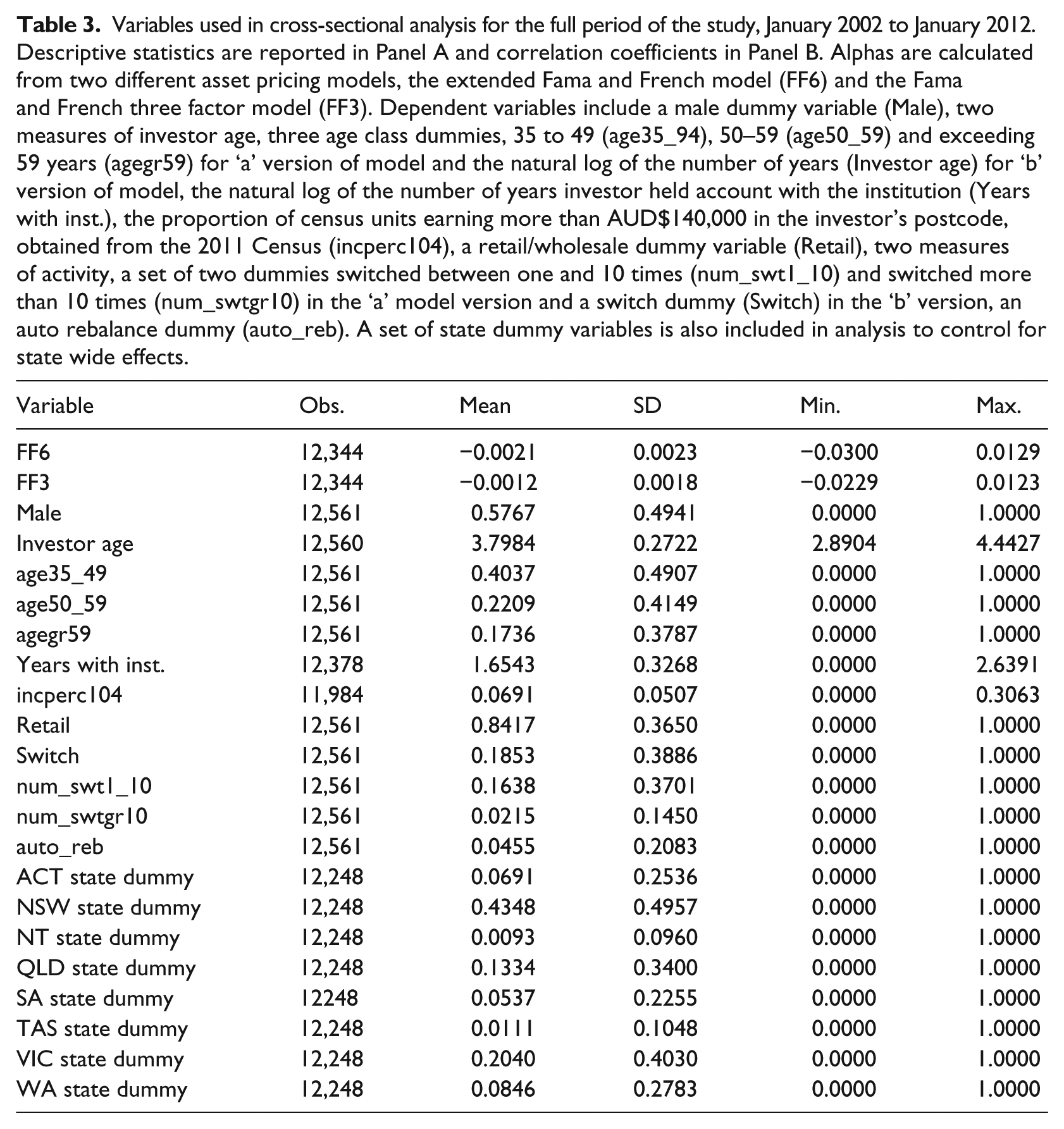
There are two measures of investor age used in the analysis. The first measure is a set of three age dummies for the age ranges 35 to 49 (age35_49), 50 to 59 (age50_59) and exceeding 59 years (agegr59). The age range dummies allow analysis to focus on particular investor age groups. There is 40% of the sample with ages falling in the range, 35 to 49, 22% in the range 50–59, 17% with ages exceeding 59 years and the remaining 21% falls in the group aged less than 35 years. The second age measure (investor age) is the natural log of the number of years from the investor birth year to the end of the study period, either 2012 for the full period or post-GFC period or 2007 for the pre-GFC period.

It is possible that individual investment performance may be related to investor knowledge and experience of the products offered by the financial institution. For our sample the average period that investors have held an account is 5.5 years though there is considerable variation in this number across the sample ranging from the minimum required 25 months’ observations through to a maximum of 14 years. In order to capture this effect we include the natural log of the number of years the investor has held their account with the financial institution (years with inst).

There is no information provided about the wealth of the investors in our data set. We expect investor wealth could have implications for investment decisions, ranging from their knowledge about investment alternatives through to their confidence in making investments and in choosing particular asset classes. We proxy wealth, using the 2011 Census postcode level income range statistics. Specifically, we use the proportion of households earning more than AUD$104,000, who live within the investor’s postcode area (incperc104), as a proxy for investor wealth. This is the maximum income level reported in the census and so we believe that individuals falling within this income range are most likely to have disposable income available for investment purposes. For the postcodes in our sample, the average proportion of households with income exceeding AUD$104,000 was 6.9% (standard deviation of 5%).

A dummy variable is also included to identify whether the investor is classified by the financial institution as a retail investor or a wholesale investor (retail). Around 84% are classified as retail superannuation fund investors and the remaining 16% are classified as wholesale superannuation investors. This variable could be important in explaining cross-sectional variation in individual investor performance as the size of an individual’s investment could reflect personal knowledge and experience along with access to special products and preferential fee structures.

Investors have the ability to switch their balance across different investment options, and hence asset classes, using either special purpose ‘switch’ transactions or through separate buy and sell transactions. This allows investors to vary their portfolio exposures over time and this ability could have implications for investment portfolio performance. Most investors (around 82%) choose not to switch asset classes over the study period but there is considerable variation in the remaining 18% that choose to switch. Around 16% of the sample falls within the range of 1 to 10 switches over the study period with just 2% switching their asset classes more than 10 times over this period. Included in this latter group is one individual who recorded 692 switches over the period from January 2002 through to January 2012. Given the highly skewed nature of switching behaviour we use a dummy variable-based measure of activity. The first measure consists of two dummy variables. The first dummy variable is set to one if the investor switched between one and 10 times during the study period (num_swt1_10), with zero otherwise. The second dummy variable is set to one if the investor switched more than 10 times during the study period (num_swtgr10), with zero otherwise. These dummy variables provide a sense of the importance of the scale of switching activity. The second of the two measures of activity is a simple switch dummy variable with a value of one if the investor switched their investments during the study period (switch) and zero otherwise.

An automatic rebalance facility is also available to investors. This allows the investor to select preferred asset classes proportions, with automatic rebalancing transactions generated over time to maintain these proportions. Only 4.5% of the investors in the sample selected this option over the study period which corresponds with the low levels of participants who manually rebalance reported by Mitchell et al. (2006). An automatic rebalance dummy variable (auto_reb) is used to capture the impact of this option on portfolio performance, with a value of one if the investor selects auto-rebalancing and zero otherwise.

Finally, a set of state dummy variables is included to control for state wide effects. ASX (2011) reports considerable variation in stock market participation across Australian states and territories. For example, in our sample, Tasmania (TAS) has the lowest stock exchange participation rate of 24% whereas New South Wales (NSW) and Western Australia (WA) have higher participation rates of 43% and 41% respectively. Differences in participation rates may signal differences in sophistication or risk preferences. Investors in the sample are distributed across six of the Australian states (NSW, Queensland (QLD), South Australia (SA), TAS, Victoria (VIC), WA) and two territories (Australian Capital Territory (ACT) and Northern Territory (NT)) and so seven state dummy variables are included in cross-sectional analysis to control for state-specific factors that may affect individual investor portfolio performance.

4. Analysis

This section reports on the results of cross-sectional analysis of investor performance as a function of member characteristics and trading behaviour. The retail and wholesale products are homogeneous with respect to the Australian taxation and government regulation and it is reasonable to use cross-sectional analysis with this data. Ordinary least squares (OLS) regression is used throughout the analysis with robust standard errors applied in calculation of probabilities reported in parentheses below the estimated coefficients. The reported analysis focuses on the alpha estimates, FF3 and FF6, which have been calculated for the full period and for the two sub-periods, pre GFC and post GFC (See Table 2 for further details).² There are two versions of the model for each of the two sets of estimated alphas (FF3 and FF6), and these two models vary with the choice of age and switch variables included in the analysis. The first model includes the age group dummy variables and the switch dummy variables, with either FF6 or FF3-based alphas used as the dependent variable $(P e r f_{i})$

P e r f_{i} = β_{0} + β_{1} m a l e_{i} + β_{21} a g e 35_49_{i} + β_{22} a g e 50_59_{i} + β_{23} a g e g r 59_{i} + β_{3} Y e a r s w i t h i n s t ._{i} + β_{4} i n c p e r c 104_{i} + β_{5} r e t a i l_{i} + β_{61} n u m_s w t 1_10_{i} + β_{62} n u m_s w t g r 10_{i} + β_{7} a u t o_r e b_{i} + \sum_{k = 1}^{7} δ_{i k} s t a t e_{i k} + ε_{i}

(3)

The second model includes the investor age and the switch dummy variable

P e r f_{i} = β_{0} + β_{1} m a l e_{i} + β_{2} I n v e s t o r a g e_{i} + β_{3} Y e a r s w i t h i n s t_{i} + β_{4} i n c p e r c 104_{i} + β_{5} r e t a i l_{i} + β_{6} s w i c t h_{i} + β_{7} a u t o_r e b_{i} + \sum_{k = 1}^{7} δ_{i k} s t a t e_{i k} + ε_{i}

(4)

The results from the cross-sectional analysis are reported in Table 4 with the results for equation (3) appearing in columns two and four and the results for equation (4) appearing in columns three and five, of Table 4.

Table 4.

Cross-section regression using performance measures.

The results from cross-section OLS regressions are reported in panels A for the full sample, Panel B for the pre-GFC sample and Panel C for the post-GFC sample. The dependent variables are alphas from an extended Fama and French model (FF6) and a Fama and French three factor model (FF3). Only those investors with at least 25 monthly return observations are included in the analysis. Independent variables include a male dummy variable (Male), two measures of investor age, three age class dummies, 35 to 49 (age35_94), 50–59 (age50_59) and exceeding 59 years (agegr59) for ‘a’ version of model and the natural log of the number of years (investor age) for ‘b’ version of model, the natural log of the number of years investor held account with the institution (Years with inst.), the proportion of investors earning more than AUD$104,000 in the investor’s postcode, obtained from the 2011 Census (incperc104), retail fund/wholesale fund dummy (Retail), two measures of activity, a set of two dummies switched between one and 10 times (num_swt1_10) and switched more than 10 times (num_swtgr10) in the ‘a’ model version and a switch dummy (Switch) in the ‘b’ version, an auto rebalance dummy (auto_reb). A set of state dummy variables is also included in all models to control for state wide effects. Robust standard errors are used in t-test calculation and probabilities are reported in parentheses below estimated coefficients. * (+) statistically significant at the 5% (10%) level.

Panel A: Full period of the study, January 2002 to January 2012.
Variable	FF6a	FF6b	FF3a	FF3b
Male	−0.000043	−0.000046	0.000003	−0.000002
	(0.30)	(0.27)	(0.92)	(0.95)
Investor age		−0.000221*		−0.000322*
		(0.01)		(0.00)
age35_49	0.000077		−0.000025
	(0.17)		(0.53)
age50_59	0.000007		−0.000096*
	(0.91)		(0.04)
agegr59	−0.000174*		−0.000282*
	(0.01)		(0.00)
Years with inst.	−0.001270*	−0.001238*	−0.000659*	−0.000637*
	(0.00)	(0.00)	(0.00)	(0.00)
incperc104	−0.000200	−0.000139	−0.000386	−0.000347
	(0.68)	(0.77)	(0.29)	(0.34)
Retail	−0.000773*	−0.000776*	−0.000542*	−0.000535*
	(0.00)	(0.00)	(0.00)	(0.00)
Switch		−0.000322*		−0.000804*
		(0.00)		(0.00)
num_swt1_10	−0.000323*		−0.000761*
	(0.00)		(0.00)
num_swtgr10	−0.000291		−0.001124*
	(0.34)		(0.00)
auto_reb	−0.000207+	−0.000202+	−0.000208*	−0.000198*
	(0.06)	(0.07)	(0.01)	(0.02)
Constant	0.000830*	0.001625*	0.000660*	0.001761*
	(0.00)	(0.00)	(0.00)	(0.00)
State dummy variables	Yes	Yes	Yes	Yes
Adjusted R square	0.05	0.05	0.05	0.05
F-statistic	31.34*	37.29*	29.11*	34.44*
Degrees of freedom	11,766	11,768	11,766	11,768
Panel B: Pre-GFC sub period, January 2002 to August 2007.
Variable	FF6a	FF6	FF3a	FF3
Male	0.000132	0.000114	0.000026	0.000004
	(0.26)	(0.33)	(0.72)	(0.96)
Investor age		0.000075		−0.000216
		(0.77)		(0.17)
age35_49	0.000256+		−0.000072
	(0.10)		(0.42)
age50_59	0.000408*		0.000115
	(0.03)		(0.32)
agegr59	−0.000068		−0.000224
	(0.76)		(0.11)
Years with inst.	−0.000751*	−0.000548+	−0.000354	−0.000284
	(0.02)	(0.08)	(0.13)	(0.22)
incperc104	0.002645*	0.002748*	0.001163	0.001126
	(0.02)	(0.02)	(0.11)	(0.13)
Retail	−0.001134*	−0.001097*	−0.000841*	−0.000791*
	(0.00)	(0.00)	(0.00)	(0.00)
Switch		−0.000116		−0.000320*
		(0.48)		(0.00)
num_swt1_10	0.000045		−0.000148
	(0.79)		(0.16)
num_swtgr10	−0.001321*		−0.001676*
	(0.00)		(0.00)
auto_reb	−0.000200	−0.000149	0.000357*	0.000376*
	(0.35)	(0.48)	(0.01)	(0.01)
Constant	−0.000486	−0.001062	0.000171	0.000717
	(0.47)	(0.39)	(0.72)	(0.36)
State dummy variables	Yes	Yes	Yes	Yes
Adjusted R square	0.05	0.03	0.06	0.04
F-statistic	5.94*	5.72*	7.41*	6.97*
Degrees of freedom	1951	1954	1951	1954
Panel C: Post-GFC sub period, September 2009 to January 2012.
Variable	FF6	FF6	FF3	FF3
Male	0.000115*	0.000102*	−0.000056	−0.000061
	(0.00)	0.00	0.11	0.09
Investor age		−0.000916*		−0.000114
		0.00		0.11
age35_49	−0.000140*		−0.000071
	(0.00)		0.14
age50_59	−0.000446*		−0.000139*
	(0.00)		0.01
agegr59	−0.000707*		−0.000044
	(0.00)		0.48
Years with inst.	0.000573*	0.000602*	−0.000039	−0.000049
	(0.00)	0.00	0.54	0.45
incperc104	0.001532*	0.001587*	−0.001473*	−0.001513*
	(0.00)	0.00	0.00	0.00
Retail	−0.001022*	−0.000997*	−0.000199*	−0.000180*
	(0.00)	0.00	0.01	0.01
Switch		−0.000765*		−0.000719*
		0.00		0.00
num_swt1_10	−0.000613*		−0.000621*
	(0.00)		0.00
num_swtgr10	−0.001957*		−0.001526*
	(0.00)		0.00
auto_reb	0.000376*	0.000403*	−0.000244*	−0.000230*
	(0.00)	0.00	0.01	0.02
Constant	0.000725*	0.003862*	0.000027	0.000390
	(0.00)	0.00	0.84	0.18
State dummy variables	Yes	Yes	Yes	Yes
Adjusted R square	0.08	0.07	0.03	0.02
F-statistic	41.57	45.83	11.05	12.98
Degrees of freedom	11,333	11,335	11,333	11,335

We first examine member demographics and socio-economic indicators. For the full period from January 2002 through to January 2012, the male dummy variable is not statistically significant. Further, while this is also statistically insignificant in the pre-GFC period it is statistically significant and positive in the post-GFC period but only for the FF6 alphas. Thus, there is no statistical support for male investors performing less well than female investors. It would appear that after adjustment for risk the gender-based performance differences, noted in the literature in this study, are limited. This is an important result as it contrasts with some of the earlier work that noted a tendency for male investors to be too active in their trading and to suffer as a result (Barber and Odean, 2001). Our sample is quite different from the US-based data and draws from a broad range of Australian investors and covers quite a volatile period. Numerous studies have noted that males have higher levels of financial literacy (Bateman et al., 2012; Lusardi and Mitchell, 2011) which makes the previous negative male-performance result surprising notwithstanding the overconfidence explanation. It may be that, for a more representative investor sample, financial literacy keeps overconfidence in check.

Investor age is significant and negatively related with individual investment alpha for the full period. Using the natural log of investor age, younger investors earn more alpha than older investors. This is further borne out with the set of age dummy variables that suggests those investors with age greater than 59 perform more poorly than the group with age less than 35 years. This result does vary with sub-period and so it is important to explore how the link between age and portfolio alpha changes between the pre-GFC and the post-GFC periods. There is little of statistical significance in the pre-GFC period with no statistically significant link evident between investor age and alpha. The only exceptions are the FF6 alpha regression-based coefficients for the age ranges 35 to 39 and 50 to 59, where it is found that these older investors appear to outperform the younger investors in the age range less than 35 years of age at the 10% level of significance or better. These results are not replicated in the Fama–French three factor model results (FF3). The results for the post GFC period are more consistent with the full period results with statistically negative results for the FF6 alpha-based analysis though the results are not so well supported with the FF3 alpha-based results. In summary, investors age had little direct impact on the portfolio performance in the pre-GFC period though it took on greater importance for the post-GFC period with evidence that older investors tended to perform more poorly in a risk-adjusted sense than the younger investors in the sample.

The number of years with the institution is negatively related with portfolio alpha for the full period and for the pre-GFC period though it is positive and significant in the post-GFC period for the FF6 alpha-based analysis. These results suggest that longer-term investors may not have been as well positioned relative to our chosen benchmark portfolios prior to the GFC though these positions may have worked better for them in the turbulence of the post-GFC period.

The investor wealth proxy (incperc104) is negative though not statistically significant in the full period analysis. This variable is quite sensitive to the alpha chosen for analysis. For both the pre-GFC and the post-GFC periods, the wealth proxy coefficients are statistically significant and positive in analysis of the FF6 alphas. Thus, investors in wealthier postcode areas tend to earn greater risk-adjusted returns than those in lower income postcode areas. The signs and significance are very much less consistent for the FF3 alpha-based analysis with statistically significant negative coefficients in the post-GFC period. One reconciliation of the contrasting signs is that those in the higher income postcodes have a more diversified portfolio which is penalised in the FF3 alpha measure but is rewarded when the broader FF6 alpha is used. Viewed this way the results support the view that wealthier individuals earned greater risk-adjusted returns both prior to and after the GFC.

We now examine investment and behaviour characteristics. Perhaps the most persistent result in the study is the finding that wholesale investors tend to outperform retail investors and this difference in performance is statistically significant in all cases, regardless of study period, variables used for age and switching and choice of alpha, FF6 or FF3. Wholesale investors are generally larger, wealthier investors and so they may have greater resources to devote to analysis which could explain the improved performance.

While switching is isolated to around 18% of the sample this activity is costly. Switching activity is invariably associated with lower risk-adjusted returns (alphas) and this is also evident across the various analyses reported in Panels A, B and C of Table 4. In this study it would appear that participants that tend to change their asset allocation over the period of the study earn lower alphas than those that do not. Virtually all of the reported coefficients are negatively signed and most are statistically significant. The statistical significance of the coefficients for the pair of switch dummy variables does exhibit some variation across the sub-periods, particularly in the pre-GFC period. In this period those with evidence of switching one to 10 times over the study period exhibit statistically insignificant coefficients while those with evidence of more than 10 switches in the period exhibit a statistically significant negative relation with the investor’s portfolio alpha. Thus, in the pre-GFC boom period those that more actively varied their portfolio earned lower risk-adjusted returns than those who chose a more stable portfolio management strategy. This result is consistent with some of the earlier literature where a negative relation between trading levels and performance (Barber and Odean, 2000b) is observed. With the post-GFC period switching, generally, is associated with lower portfolio alpha.

The final variable that is included in the paper is a dummy variable to capture the impact of the automatic rebalancing option that is available to investors. The results are sensitive to performance measure and period analysed. Over the whole period a significant negative result is estimated which masks different results in the two sub-periods. In the pre-GFC period auto-rebalancing has a positive result when using the FF3, which is surprising given the positive equity markets. In the post-GFC period auto-rebalancing has a positive (negative) result using the FF6 (FF3) performance measure. The result can be contrasted with Mitchell et al. (2006) who find a positive benefit of rebalancing but it is important to note the different measures of rebalancing employed in the current study and Mitchell et al. (2006). We include those who include a passive rebalance option. That is, investors who select an option requiring the institution to rebalance on their behalf whereas Mitchell et al. (2006) instead identify rebalancing as reflected in the actual choice of the investor returning to a previous asset allocation. The result may be influenced by the small proportion of accounts that opt for rebalancing but that is also the case for Mitchell et al. (2006). This result warrants further research though this is beyond the scope of the present study.

5. Conclusions

Saving for retirement requires a solution to the interdependent questions of how much to save and how to save or invest. We have examined the second problem using a new sample of individual transaction histories covering an extended period of time (2002–2012) within a superannuation product for discretionary retirement savings offered by a large Australian financial institution. The question has direct importance for individuals due to its consequences for standard of living in retirement. It also has importance for taxpayers who provide tax concessions to these savings in the expectation that the demand on the public purse will be commensurately reduced in retirement.

Our results provide corroborating evidence to previous international evidence with noted differences. Before discussing results it is important to note that the performance measure employed is important as results for some variables are sensitive to whether the ‘standard’ three-factor Fama–French model is employed or an augmented Fama–French model which incorporates exposure to fixed interest and property asset classes which better reflect the risk factors individuals face.

A stylised summary of the results suggests performance is reduced through high levels of trading, for retail investors and with some evidence suggesting an age penalty as well, isolated to the post-GFC period. Investors in higher income suburbs also do better though this result is not consistent by performance measure which we speculate is due to the more diversified portfolios that wealthier investors hold. We do not find support for gender differences in performance which contrasts with previous literature where males have underperformed. The role of auto-rebalancing is mixed, sensitive to performance measure and period. A small proportion of investors select this option as an automatic service but further research could provide greater insight as to those who auto-rebalance manually.

Finally, while the proportion of investors who actually trade is larger than reported for mandatory retirement savings accounts (Clark-Murphy and Gerrans, 2001; Gerrans, 2012), it remains surprisingly low at 18% overall. However, given the generally negative impact of trading activity, we should note the underlying wisdom of the majority in choosing not to adjust their portfolio on a regular basis.

Footnotes

Acknowledgements

We thank the financial institution who made the extensive transaction database available and Jacqui Whale who completed the task of constructing the database from the data.

Final transcript accepted 23 February 2014 by Garry Twite (AE Finance).

Funding

This research received no specific grant from any funding agency in the public, commercial, or not-for-profit sectors.

1.

The estimate of the mean return per annum, given the mean return for the month, $μ_{M}$ , is $μ_{Y} = μ_{M} * 1200$ . The estimate of the standard deviation per annum, given the standard deviation for the month, $σ_{M}$ , is $σ_{Y} = σ_{M} * \sqrt{12} * 100$

2.

As a robustness test we have also replicated this analysis using Jensen alphas and alphas from an extended Jensen model (with added international returns, Australian retail returns and Australian fixed interest returns) not reported separately here, and find there is little difference in the final results between the Jensen and the FF3 analysis and between the extended Jensen model alpha and the FF6 analysis.

References

Anderson

Gerlach

DiTraglia

(2007) Yes, Wall Street, there is a January effect! Evidence from laboratory auctions. The Journal of Behavioral Finance 8: 1–8.

Australian Prudential Regulation Authority (2013) Quarterly Superannuation Performance. Sydney, VIC, Australia: Australian Prudential Regulation Authority.

Australian Securities Exchange (ASX) (2011) 2010 Australian Share Ownership Study. Sydney, VIC, Australia: Australian Securities Exchange.

Barber

Odean

(2000a) Too many cooks spoil the profits: Investment club performance. Financial Analysts Journal 56: 17–25.

Barber

Odean

(2000b) Trading is hazardous to your wealth: The common stock investment performance of individual investors. Journal of Finance 55: 773–806.

Barber

Odean

(2001) Boys will be boys: Gender, overconfidence, and common stock investment. The Quarterly Journal of Economics 116: 261–292.

Barber

Odean

(2002) Online investors: Do the slow die first? Review of Financial Studies 15: 455–487.

Barber

Odean

(2008) All that glitters: The effect of attention and news on the buying behavior of individual and institutional investors. Review of Financial Studies 21: 785–818.

Barber

Heath

Odean

(2003) Good reasons sell: Reason-based choice among group and individual investors in the stock market. Management Science 49: 1636–1652.

10.

Barber

Lee

Y-T

Liu

Y-J

. (2009) Just how much do individual investors lose by trading? Review of Financial Studies 22: 609–632.

11.

Bateman

Eckert

Geweke

. (2012) Financial competence and expectations formula: Evidence from Australia. The Economic Record 88: 39–63.

12.

Benartzi

(2001) Excessive extrapolation and the allocation of 401(k) accounts to company stock. Journal of Finance 56: 1747–1764.

13.

Bernatzi

Thaler

(1995) Myopic loss aversion and the equity puzzle. Quarterly Journal of Economics 110: 73–92.

14.

Bhattacharya

Hackethal

Kaesler

. (2012) Is unbiased financial advice to retail investors sufficient? Answers from a large field study. Review of Financial Studies 25: 975–1032.

15.

Bird

Chin

McCrae

(1983) The performance of Australian superannuation funds. Australian Journal of Management 8: 49–69.

16.

Busse

Goyal

Wahal

(2010) Performance and persistence in institutional investment management. Journal of Finance 65: 765–790.

17.

Calvet

Campbell

Sodini

(2006) Down or out: Assessing the welfare costs of household investment mistakes. NBER Working Paper No. 12030. Cambridge, MA: National Bureau of Economic Research.

18.

Choi

Laibson

Madrian

. (2002) Defined contribution pensions: Plan rules, participant decisions, and the path of least resistance. In: Porteba

(ed.) Tax Policy and the Economy. Cambridge, MA: MIT Press. pp. 67–114.

19.

Clark-Murphy

Gerrans

(2001) Choices and retirement savings: Some preliminary results on superannuation fund member decisions. Economic Papers 20: 29–42.

20.

Clark-Murphy

Soutar

(2004) What individual investors value: Some Australian evidence. Journal of Economic Psychology 25: 539–555.

21.

Clark-Murphy

Gerrans

Speelman

(2009) Drivers of individuals’ superannuation investment choices: Preliminary evidence on return chasing and demographics. Journal of Family and Economic Issues 30: 4–19.

22.

Clark-Murphy

Kristofferson

Gerrans

(2002) What makes superannuation decisions difficult? International Journal of Business Studies 10: 73–94.

23.

Commonwealth of Australia (2010) Stronger Super Canberra, ACT, Australia: Commonwealth of Australia.

24.

Cummings

(2012) Effect of Fund Size on the Performance of Australian Superannuation Funds. Sydney, VIC, Australia: Australian Prudential Regulation Authority.

25.

Cummings

Ellis

(2011) Risk and Return of Illiquid Investments: A Trade-Off for Superannuation Funds Offering Transferable Accounts. Sydney VIC, Australia: Australian Prudential Regulation Authority.

26.

Drew

(2006) Superannuation: Switching and roulette wheels. Australian Accounting Review 16: 23–31.

27.

Faff

(2001) An examination of the Fama and French three-factor model using commercially available factors. Australian Journal of Management 26: 1–17.

28.

Fama

French

(1993) Common risk factors in the returns on stocks and bonds. Journal of Financial Economics 33: 3–56.

29.

Fama

French

(2010) Luck versus skill in the cross-section of mutual fund returns. Journal of Finance 65: 1915–1947.

30.

Fry

Heaney

McKeown

(2007) Will investors change their superannuation fund given the choice? Accounting and Finance 47: 267–283.

31.

Gallagher

(2001) Attribution of investment performance: An analysis of Australian pooled superannuation funds. Accounting and Finance 41: 41–62.

32.

Gallagher

Jarnecic

(2002) The performance of active Australian bond funds. Australian Journal of Management 27: 163–185.

33.

Gallagher

(2003) Investment manager characteristics, strategy, top management changes and fund performance. Accounting and Finance 43: 283–309.

34.

Gerrans

(2012) Retirement savings investment choices in response to the global financial crisis: Australian evidence. Australian Journal of Management 37: 415–439.

35.

Gerrans

Clark

(2013) Pension plan participant choice: Evidence on defined benefit and defined contribution preference. Journal of Pension Economics & Finance 12: 351–378.

36.

Gerrans

Clark-Murphy

Speelman

(2008) Retirement savings investment strategy: Member choices and performance. In: Proceedings of the 16th annual colloquium of superannuation researchers, UNSW, Sydney, NSW, Australia.

37.

Gharghori

Mudumbab

Veeraraghavan

(2007) How smart is money? An investigation into investor behaviour in the Australian managed fund industry. Pacific-Basin Finance Journal 15: 494–513.

38.

Gharghori

Sujoto

Veeraraghavan

(2008) Are Australian investors smart. Australian Journal of Management 32: 525–544.

39.

Grinblatt

Keloharju

(2001a) How distance, language, and culture influence stockholdings and trades. Journal of Finance 56: 1053–1073.

40.

Grinblatt

Keloharju

(2001b) What makes investors trade? Journal of Finance 56: 589–616.

41.

Gruber

(1996) Another puzzle: The growth in actively managed mutual funds. Journal of Finance 51: 783–810.

42.

Guiso

Jappelli

(2006) Information acquisition and portfolio performance. CEPR Discussion Paper no. 5901. London: Centre for Economic Policy Research.

43.

Hackethal

Haliassos

Jappelli

(2012) Financial advisors: A case of babysitters? Journal of Banking & Finance 36: 509–524.

44.

Haigh

List

(2005) Do professional traders exhibit myopic loss aversion? An experimental analysis. Journal of Finance 60: 523–534.

45.

Hedesstrom

Svedsater

Garling

(2004) Identifying heuristic choice rules in the Swedish premium pension scheme. The Journal of Behavioral Finance 5: 32–42.

46.

Holmes

Faff

(2004) Stability, asymmetry and seasonality of fund performance: An analysis of Australian multi-sector managed funds. Journal of Business Finance & Accounting 31: 539–578.

47.

Holmes

Faff

(2008) Estimating the performance attributes of Australian multi-sector managed funds within a dynamic Kalman filter framework. International Review of Financial Analysis 17: 998–1011.

48.

Kim

(2013) On timing ability in Australian managed funds. Australian Journal of Management. Epub ahead of print 22 January 2013.

49.

Jones

van der Laan

Frost

. (2008) The investment performance of socially responsible investment funds in Australia. Journal of Business Ethics 80: 181–203.

50.

Kahneman

Tversky

(1984) Choices, values, and frames. American Psychologist 39: 341–350.

51.

Kahneman

Knetsch

Thaler

(1991) The endowment effect, loss aversion, and status quo bias. Journal of Economic Perspectives 5: 193–206.

52.

Kluger

Wyatt

(2004) Are judgment errors reflected in market prices and allocations? Experimental evidence based on the Monty Hall Problem. Journal of Finance 59: 969–998.

53.

Lewellen

Lease

Schlarbaum

(1977) Patterns of investment strategy and behavior among individual investors. Journal of Business 50: 296–333.

54.

Repin

Steenbarger

(2005) Fear and greed in financial markets: A clinical study of day-traders. American Economic Review 95: 352–359.

55.

Lusardi

Mitchell

(2011) Financial literacy around the world: An overview. Journal of Pension Economics & Finance 10: 497–508.

56.

Malkiel

(2005) Reflections on the efficient market hypothesis: 30 years later. The Financial Review 40: 1–9.

57.

Medcraft

(2012) Speech to Conference of Major Superannuation Funds. Conference of Major Superannuation Funds, Southbank, Brisbane, QLD, Australia.

58.

Mitchell

Mottola

Utkus

. (2006) The inattentive participant: Portfolio trading behavior in 401(k) plans. Working Paper No. 2006–5. Ann Arbor, MI: Michigan Retirement Research Center, University of Michigan.

59.

Odean

(1998) Are investors reluctant to realise their losses? Journal of Finance 53: 1775–1798.

60.

Pinnuck

(2004) An examination of the performance of the trades and stock holdings of fund managers: Further evidence. Journal of Financial and Quantitative Analysis 38: 811–828.

61.

Porter

Smith

(2003) Stock market bubbles in the laboratory. The Journal of Behavioral Finance 4: 7–20.

62.

Sapp

Tiwari

(2004) Does stock return momentum explain the ‘smart money’ effect? Journal of Finance 59: 2605–2622.

63.

Sinclair

(1990) Market timing ability of pooled superannuation funds January 1981 to December 1987. Accounting and Finance 30: 51–65.

64.

Tang

Mitchell

Mottola

. (2009) The efficiency of sponsor and participant portfolio choices in 401(k) plans. Pension Research Council Working Paper PRC WP2009-08. Philadelphia, PA: The Wharton School, The University of Pennsylvania.

65.

Thaler

(1999) Mental accounting matters. Journal of Behavioral Decision Making 12: 183–206.

66.

Yamaguchi

Mitchell

Mottola

. (2006) Winners and losers: 401(k) trading and portfolio performance. Pension Research Council Working Paper WP2006-26. Philadelphia, PA: The Wharton School, University of Pennsylvania.