Probability of loss reversal in Australia

1. Introduction

The percentage of Australian listed firms reporting annual accounting losses has been consistently above 40% and increasing over the past two decades (Balkrishna et al., 2007; Wu et al., 2010). This persistently large proportion of listed firms reporting losses is surprising since permanent losses should trigger abandonment (Burgstahler and Dichev, 1997; Hayn, 1995). Survival thus implies a market expectation that losses will be transitory and loss firms will eventually become profitable (loss reversal). Assessing the probability of loss reversal is likely to be critical to investors’ abandonment and valuation decisions (Joos and Plesko, 2005). Following this appraisal, whether and how investors assess the probability of loss reversal when valuing loss firms are important empirical questions (Li, 2011). This article examines the accounting information associated with the likelihood of loss reversal in Australian firms. It further examines the investor use of this information in pricing loss firms.

The objectives of this article are threefold. First, Joos and Plesko (2005) develop a model (the JP model) to predict 1-year-ahead loss reversal using the past and current accounting information of US firms. This article examines whether the factors included in the JP model are also useful in the Australian context. Second, prior research shows that high investment intensity is associated with the increasing incidence of losses (Darrough and Ye, 2007; Klein and Marquardt, 2006; Wu et al., 2010). Extending the JP model, I explore the implications of investment activity for future loss reversal.

The article’s third objective is to use the extended JP model to construct a measure of the ex-ante likelihood of loss reversal. I then examine whether this probability measure is associated with loss firms’ future abnormal stock performances. This approach is motivated by recent evidence suggesting that investors may not fully anticipate the valuation implications of accounting information for loss firms (Balakrishnan et al., 2010; Dhaliwal et al., 2013; Jiang et al., 2016; Li, 2011). Prior studies point to the lower earnings persistence of losses compared to profits (Hayn, 1995) as a source of difficulty for investors in making valuation adjustments based on publicly available information. ¹ If investors do not fully process reported financial information, one would expect the predicted probability of loss reversal to be useful in explaining future abnormal stock returns.

I examine a sample of loss firms for the period 1993 through 2010; the results show that loss firms’ current and past performances, loss patterns and signals contained in dividend payments are useful for predicting future loss reversal in Australia. ² Firms’ reported income tax and deferred tax items are also related to future loss reversal (Dhaliwal et al., 2013). More importantly, loss firms reporting a high level of investment in specialised assets, ³ including mineral exploration and research and development (R&D), relative to fixed-asset investment are more likely to experience persistent losses in the near future. In contrast, a high level of fixed-asset investment indicates an increase in the probability of future loss reversal. This is consistent with loss firms experiencing differing likelihoods of loss reversal in different stages of their investment cycle. In the early stage of investment, firms engage in more specialised investment activities and revenues are less likely to be generated in the near future. When firms move into a later stage of investment, they acquire more fixed assets in preparation for future production. Loss reversal thus becomes more achievable.

Regarding the third research objective, I relate the predicted probability of loss reversal to future abnormal returns. The results show that loss firms with a low probability of loss reversal (persistent loss) experience significantly more negative abnormal returns than firms with a high probability of loss reversal (transitory loss). A zero-investment hedge portfolio taking a long position in a transitory-loss portfolio and a short position in a persistent-loss portfolio generates a statistically significant annual buy-and-hold abnormal return (BHAR) of 21.2% (equal weighted, 12.9% for value weighted) before transaction costs. Further analysis shows that the association between the predicted probability of loss reversal and future abnormal returns is observed only in loss firms with no analyst following and loss firms not included in the ASX 200 index. Investors in these loss firms are likely to face a weaker information environment and may hence find it difficult to fully process the signals contained in accounting information (Dhaliwal et al., 2013). The accounting factors examined in this article are most useful for investors in loss firms with a weak information environment.

This article makes two contributions. First, it extends the literature to show that firms’ investment activities are useful in explaining the likelihood of future loss reversal. Given that this factor is prevalent among loss firms, this article assists loss-firm investors in interpreting the implications of investment activities for future profitability. Furthermore, due to their association with different stages of the investment cycle, different types of investment hold different implications for future loss reversal. Investors should assess firms’ investment mix of specialised and fixed assets when valuing loss firms.

Second, the results have implications for loss-firm valuation in Australia. While prior literature examines whether Australian investors incorporate the various accounting factors in loss-firm valuation (Sin and Watts, 2000; Wu et al., 2010), this research focuses on examining how Australian investors incorporate these accounting factors in pricing loss firms. It finds that investors’ ability to interpret accounting information when pricing loss firms varies with the firm information environment. Specifically, the results suggest that investors may not be efficient at pricing loss firms with a weak information environment. This research provides investors in Australian loss firms with guidance on how to incorporate reported information when assessing future profitability.

This article proceeds as follows. The literature is reviewed next. Section 3 develops the hypotheses. Section 4 describes the research design, followed by a section describing the sample. Section 6 reports the results. The final section concludes.

2. Literature review

Research interest in the probability of loss reversal originates with Hayn (1995), who suggests that the insignificant association between losses and contemporaneous stock returns may be due to the high likelihood of investors abandoning loss firms. If a firm is expected to suffer losses indefinitely, investors should liquidate the firm and redeploy resources (Burgstahler and Dichev, 1997; Hayn, 1995). It follows that the expectation maintained for a surviving loss firm is that it will eventually become profitable. Therefore, assessing the probability of loss reversal is useful for investors deciding on whether to abandon the firm (Joos and Plesko, 2005).

Sin and Watts (2000) examine the valuation of loss firms in Australia. They argue that, for firms that subsequently become profitable, investors are more likely to treat losses as transitory earnings. The authors find that the association between earnings and stock returns is significantly lower for loss firms that experience ex-post loss reversal. Joos and Plesko (2005) assess the ex-ante probability of loss reversal for loss firms in the US context and find that a parsimonious set of financial variables is useful for predicting future loss reversal. More importantly, they show that investors value persistent-loss and transitory-loss firms differently, suggesting that assessing the ex-ante likelihood of loss reversal is useful for valuation.

While the literature indicates that future loss reversal is associated with factors that also explain loss incidence (e.g. firm size and firm performance), several other loss-related characteristics may also hold implications for assessing loss reversal. Darrough and Ye (2007) show that many loss firms in a knowledge-based economy engage in intensive, specialised investments, such as R&D. These authors demonstrate that loss firms with high R&D investments are likely to report losses for longer periods. Wu et al. (2010) show that resource firms investing heavily in mineral exploration projects dominate Australian loss firms. Given the prevalence of investment activity among loss firms, this research examines the implications of different types of investment for the likelihood of future loss reversal.

Recent research focuses on whether investors predict future earnings efficiently when valuing loss firms. Li (2011) develops an earnings forecast model based on the JP model. The author finds evidence suggesting that the market does not fully distinguish persistent-loss firms from transitory-loss firms. Jiang et al. (2016) find similar results in the UK market. Dhaliwal et al. (2013) find that future abnormal stock returns are associated with tax items for loss firms with a weak information environment, ⁴ suggesting that investors initially underestimate the positive signals contained in these tax items. Balakrishnan et al. (2010) find evidence consistent with investors underestimating the persistence of extreme losses. The above results indicate that investors may find it difficult to assess the persistence of losses. In addition, loss persistence is closely related to special items, which reflect the transitory component of earnings (Darrough and Ye, 2007). There is also evidence suggesting that investors do not fully understand the implications of negative special items for future earnings (Burgstahler et al., 2002; Dechow and Ge, 2006). This casts further doubt on investors’ ability to estimate the probability of loss reversal. My research provides evidence on how Australian investors price signals of future loss reversal.

3. Hypothesis development

I first develop a hypothesis in relation to the impact of loss firms’ investment activity on their likelihood of future profitability. I then develop a hypothesis regarding the relation between an ex-ante measure of probability of loss reversal and future BHARs.

The literature typically recognises high investment outlays as a prominent characteristic of loss firms (Darrough and Ye, 2007; Franzen and Radhakrishnan, 2009; Wu et al., 2010). The persistence of losses is likely to vary depending on the types of investment undertaken at different investment stages. Many Australian loss firms are start-ups investing heavily in specialised assets, such as R&D or mineral exploration, since they aim to develop new products or discover commercially viable mineral resources (Darrough and Ye, 2007; Wu et al., 2010). For such firms in the early stage of investment, losses may persist for two reasons. First, the benefits of the specialised assets typically take multiple periods to realise. For example, for pharmaceutical R&D projects, the average period between drug discovery and Food and Drug Administration approval is 14.2 years (DiMasi, 2001). Investment in mineral exploration is also likely to face a rather lengthy investment cycle. Second, because of the long investment horizon, investment in specialised assets is likely to require substantial subsequent outlays. Before these investments can reach the commercialisation stage, losses are likely to persist due to lower revenue and subsequent expenditures.

Unlike specialised assets, a high level of investment in fixed assets, such as property, plant and equipment (PPE) may indicate transitory losses. Fixed assets are typically used in supporting production, logistics and sales. These activities increase with the anticipation of future revenue. In progressing from the investment phase to the commercialisation phase, firms are likely to move away from investing in specialised assets and towards fixed assets. ⁵ Loss firms’ allocation of greater resources to fixed assets may thus signal a higher probability of loss reversal in the near future. The above discussion suggests that the likelihood of future loss reversal varies with the relative level of specialised and fixed-asset investments, indicating different stages of the investment cycle, as predicted in the following hypothesis:

This research uses the JP model and its extensions to examine the relation between various accounting factors and future loss reversal. If these accounting factors are useful in distinguishing persistent-loss firms from transitory-loss firms, then an efficient market should correctly incorporate these factors in the stock price. In such case, the predicted probability of loss reversal based on the JP model should exhibit no relation with future abnormal returns. However, if investors do not fully understand the implication of accounting information for future profitability, this may result in mispricing.

Mispricing can occur under two scenarios. First, if investors expect future earnings to follow a random walk process and treat all losses as persistent, they will undervalue firms with a high probability of loss reversal (transitory-loss firms). Alternatively, if investors expect all losses to be temporary (Balakrishnan et al., 2010; Hayn, 1995), they will underestimate the persistence of loss for firms with a low probability of loss reversal and hence overvalue persistent-loss firms. Under both scenarios, when loss reversals are realised, investors will experience differing stock performance with different levels of ex-ante probability of loss reversal. Evidence from the US market is consistent with the market inefficiently assessing the probability of loss reversal (Dhaliwal et al., 2013; Li, 2011). Furthermore, Sin and Watts (2000) find market response to earnings to be weaker for Australian firms with more persistent loss. This evidence can be interpreted as Australian investors underreacting to persistent losses. The above discussion leads to the following hypothesis:

4. Research design

4.1. Modelling loss reversal

To examine H1, the JP model is adopted and extended, where 1-year-ahead loss reversal is modelled on current and past accounting information, as follows

LossRev i , t + 1 = α 1 SpeInv _ FA i , t + α 2 ACC i , t + α 3 PACC i , t + α 4 CFO i , t + α 5 PCFO i , t + α 6 SIZE i , t + α 7 SG i , t + α 8 FirstLoss i , t + α 9 LossSeq i , t + α 10 DIV i , t + α 11 DIVSTOP i , t + α 12 ITE i , t + α 13 DTA i , t + α 14 DTL i , t + ε i , t + 1

(1)

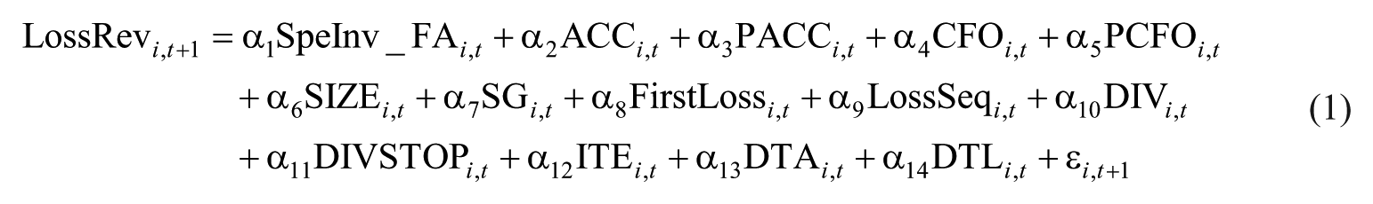
where

LossRev_i,t + 1 is an indicator variable that equals one if loss firm i reports positive net profit after tax before abnormal items in year t + 1(NPAT_i,t + 1 > 0) and zero otherwise; SpeInv_FA _i,t is the ratio of specialised assets to fixed assets (FixedAssets _i,t ) at the end of year t, with specialised assets as the sum of capitalised exploration (EXPL _i,t ) and R&D expenditures (R&D _i,t ); EXPL _i,t is the exploration expenditure capitalised at the end of year t (Datalink item #458); R&D _i,t is the estimated net R&D assets after adjusting for capitalisation and the amortisation of R&D expenses; ⁶ FixedAssets _i,t is the reported net fixed assets in year t (Datalink item #5030); NPAT _i,t is the earnings, measured as net profit after tax before abnormal items (Datalink item # 8020) in year t; ACC _i,t is a measure of accruals, defined as earnings (NPAT _i,t ) minus cash flows from operations (CFO _i,t , Datalink item #9100) in year t; PACC _i,t is the average past accruals, defined as the average value of past ACC _i,t , covering a period from 3 years to a maximum of 5 years; CFO _i,t is the cash flows from operations (Datalink item #9100) in year t; PCFO _i,t is the average past cash flows, defined as the average value of past CFO _i,t , covering a period from 3 years to a maximum of 5 years; SIZE _i,t is a measure of firm size, defined as the natural log of total market capitalisation 3 months after the end of financial year t; SG _i,t is the percentage change in trading revenue (Datalink item #7010) in year t; FirstLoss _i,t is an indicator variable that equals one if the current year’s loss is the first in a sequence and zero otherwise; LossSeq _i,t is the loss sequence, equal to the number of reported losses divided by the number of earnings observed in the past 3–5 years; DIV _i,t is an indicator variable equal to one if the company pays dividends in the current year t and zero otherwise; DIVSTOP _i,t is an indicator variable equal to one if the company stops paying dividends in the current year t and zero otherwise; ITE _i,t is the total income tax expenses (Datalink item #8035) in year t; DTA _i,t is an indicator variable that equals one if the company reports positive deferred tax assets (Datalink item #457) in year t and zero otherwise; DTL _i,t is an indicator variable that equals one if the company reports positive deferred tax liabilities (Datalink item #366) in year t and zero otherwise; and TA_{i,t − 1} is the total assets at the end of year t − 1 (Datalink item #5090).

All the variables except for SpeInv_FA _i,t , SIZE _i,t , SG _i,t , LossSeq _i,t and the indicator variables are scaled by TA_{i,t − 1}. The dependent variable is loss reversal in year t + 1. Equation (1) includes a variable measuring the relative level of specialised investments to fixed-asset investment (SpeInv_FA _i,t ). Since mineral exploration and R&D are the most common forms of investment in Australia (Wu et al., 2010), a specialised investment includes these two types of investments. According to H1, the coefficient of SpeInv_FA _i,t is expected to be significantly negative. I also examine the effect of specialised investment and fixed-asset investment on future loss reversal separately by replacing SpeInv_FA _i,t with exploration assets (EXPL _i,t ), R&D assets (R&D _i,t ) and fixed assets (FixedAssets _i,t ).

Apart from the variables measuring loss firms’ investment activities, the original variables in the JP model are included. Measures of current year performance (ACC _i,t , CFO _i,t ) are expected to be positively associated with loss reversal, that is, firms incurring smaller losses are more likely to return to profitability than firms incurring larger losses. Similarly, past performance (PACC _i,t , PCFO _i,t ) is expected to be positively related to loss reversal. ⁷ Firm size (SIZE _i,t ) is expected to be positively associated with loss reversal, since larger firms are more likely to experience temporary losses (Joos and Plesko, 2005). If a firm is making its first loss in a sequence (FirstLoss _i,t ), the current loss is more likely to be temporary. A higher frequency of losses observed in past years (LossSeq _i,t ) indicates more persistent losses. In addition, higher dividend payments (DIV _i,t ) could signal brighter financial prospects. Conversely, when a firm stops paying dividends (DIVSTOP _i,t ), investors expect a lower likelihood of future loss reversal. Motivated by Dhaliwal et al. (2013), I include three tax items to capture signals of positive current taxable income (ITE _i,t ), future tax benefits (DTA _i,t ) and future tax losses (DTL _i,t ), which indicate expected positive future incomes. These three variables are expected to be positively associated with future loss reversal.

4.2. Predicted probability of loss reversal and future BHAR

Hypothesis H2 relates an ex-ante probability of loss reversal to future BHARs. I use equation (1) as a framework for constructing an ex-ante measure of probability of loss reversal. Specifically, I estimate equation (1) on a yearly basis and then apply the previous year’s estimated coefficients to current year data. The fitted value is the predicted probability of loss reversal. I calculate BHAR_i,t + 1 as monthly abnormal returns accumulated for a 12-month period, starting from 3 months after the end of financial year t. ⁸

To test H2, two research designs are used. In the portfolio approach, loss observations are partitioned into four portfolios by their predicted probability of loss reversal on a yearly basis. The persistent-loss (transitory-loss) sample contains observations in the lowest (highest) quartile, which are the least (most) likely to reverse. I examine the mean BHAR_i,t + 1 of annual zero-investment hedge portfolios that take a long position in the transitory-loss portfolio and an equal-value short position in the persistent-loss portfolio. If investors fail to distinguish between these two types of loss firms effectively, I expect to find a significantly positive mean return for the hedge portfolios.

The second method employs regression modelling. Here, BHAR_i,t + 1 is regressed on the predicted probability of loss reversal. I control for the effect of earnings (Balakrishnan et al., 2010), accruals (Sloan, 1996), stock volatility and dividend payments. Because reversal loss firms are less likely to face bankruptcy, the probability of loss reversal may simply capture the effect of probability of bankruptcy. I also include a variable measuring distress risk (ZScore _i,t ). The model is as follows

BHAR i , t + 1 = β 0 + β 1 Rplorev i , t + β 2 NPAT i , t + β 3 ACC i , t + β 4 VOL i , t + β 5 DIV i , t + β 6 ZScore i , t + ε i , t + 1

(2)

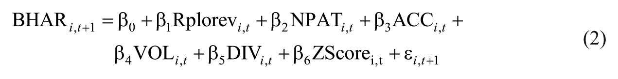
where Rplorev _i,t is the quartile ranking of the predicted probability of loss reversal for firm i in year t; NPAT _i,t is the net profit after tax before abnormal items (Datalink item # 8020) in year t; ACC _i,t is a measure of accruals, defined as earnings (NPAT _i,t ) minus cash flows from operations (CFO _i,t , Datalink item #9100) in year t; VOL _i,t is the standard deviation of monthly returns over a 12-month period ended 3 months after the end of financial year t for firm i; DIV _i,t is an indicator variable that equals one if the firm pays dividends in the current year t and zero otherwise; and ZScore _i,t is the Altman’s Z-score for firm i in year t. ⁹

Equation (2) is estimated with standard errors clustered by firm and year. The coefficient of Rplorev _i,t is expected to be significantly positive.

5. Sample and descriptive statistics

Financial data are sourced from the Morningstar Datalink database. Stock return data are from the Share Price and Price Relative database. Based on the intersection between these two databases, several selection criteria are imposed. First, this study examines up to a 3-year-ahead loss reversal. The latest sampling year is 2010. ¹⁰ Second, observations with missing lagged total assets, lagged total equity and fixed assets are excluded. These data are required for scaling. Third, I define earnings as net profit after tax before abnormal items (NPAT _i,t ) and delete all observations with a positive NPAT _i,t . After excluding observations with missing income tax expense data, the final sample contains 8406 firm-year observations (1405 unique firms) for the period 1993–2010.

Table 1 presents the yearly sample distributions. Column A shows that the frequency of loss firms increases from 261 observations in 1993 to 448 observations in 2010. I define loss reversal firms as those that report positive earnings in year t + 1. ¹¹ Column C shows that, on average, only 13.74% of loss firms become profitable in year t + 1. It appears that losses are quite persistent in Australia. Unreported results show that around 30% of loss firms revert to profit in the 3 years following losses. Columns E and G indicate that resource-based loss firms experience a smaller percentage of loss reversal than non-resource loss firms do. This suggests potential differences between resource-based and non-resource loss firms. I separately examine these two types of firms in section 6.3.

OPEN IN VIEWER

Table 1.

Yearly frequencies of loss-reversal and non-reversal firms, exploration firms.

Year	Yearly loss sample	Non-reversal	Reversal	Resource firms		Non-resource firms
	A	B	C	Non-reversal	Reversal	Non-reversal	Reversal
				D	E	F	G
1993	261	197	64	145	20	52	44
		75.48%	24.52%	87.88%	12.12%	54.17%	45.83%
1994	256	219	37	171	18	48	19
		85.55%	14.45%	90.48%	9.52%	71.64%	28.36%
1995	304	251	53	172	29	79	24
		82.57%	17.43%	85.57%	14.43%	76.70%	23.30%
1996	356	301	55	203	21	98	34
		84.55%	15.45%	90.63%	9.38%	74.24%	25.76%
1997	362	313	49	219	23	94	26
		86.46%	13.54%	90.50%	9.50%	78.33%	21.67%
1998	353	312	41	222	16	90	25
		88.39%	11.61%	93.28%	6.72%	78.26%	21.74%
1999	401	342	59	235	32	107	27
		85.29%	14.71%	88.01%	11.99%	79.85%	20.15%
2000	431	389	42	219	20	170	22
		90.26%	9.74%	91.63%	8.37%	88.54%	11.46%
2001	530	475	55	211	19	264	36
		89.62%	10.38%	91.74%	8.26%	88.00%	12.00%
2002	578	491	87	227	23	264	64
		84.95%	15.05%	90.80%	9.20%	80.49%	19.51%
2003	560	466	94	242	19	224	75
		83.21%	16.79%	92.72%	7.28%	74.92%	25.08%
2004	526	473	53	255	18	218	35
		89.92%	10.08%	93.41%	6.59%	86.17%	13.83%
2005	564	476	88	268	36	208	52
		84.40%	15.60%	88.16%	11.84%	80.00%	20.00%
2006	603	527	76	303	32	224	44
		87.40%	12.60%	90.45%	9.55%	83.58%	16.42%
2007	724	623	101	379	43	244	58
		86.05%	13.95%	89.81%	10.19%	80.79%	19.21%
2008	578	525	53	350	21	175	32
		90.83%	9.17%	94.34%	5.66%	84.54%	15.46%
2009	571	481	90	333	40	148	50
		84.24%	15.76%	89.28%	10.72%	74.75%	25.25%
2010	448	390	58	271	35	119	23
		87.05%	12.95%	88.56%	11.44%	83.80%	16.20%
Total	8406	7251	1155	4425	465	2826	690
		86.26%	13.74%	90.49%	9.51%	80.38%	19.62%

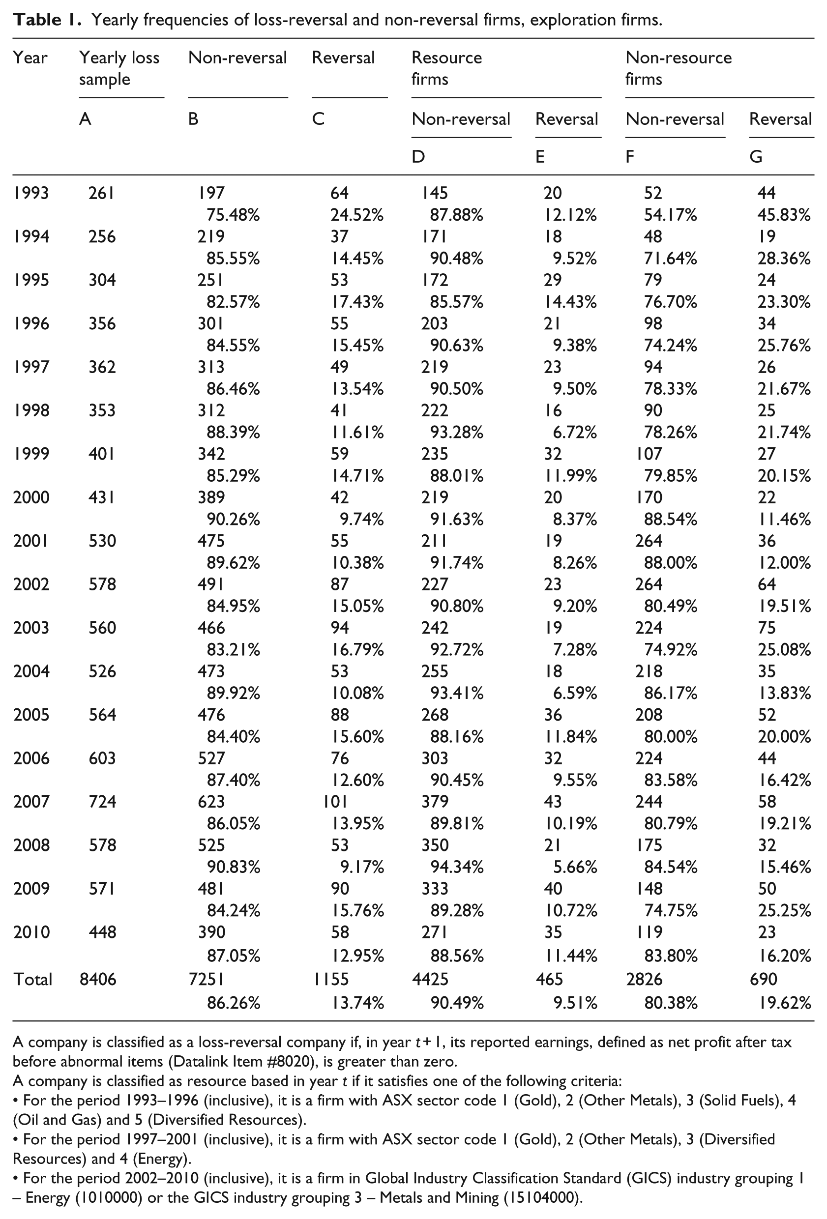
A company is classified as a loss-reversal company if, in year t + 1, its reported earnings, defined as net profit after tax before abnormal items (Datalink Item #8020), is greater than zero.

A company is classified as resource based in year t if it satisfies one of the following criteria:

• For the period 1993–1996 (inclusive), it is a firm with ASX sector code 1 (Gold), 2 (Other Metals), 3 (Solid Fuels), 4 (Oil and Gas) and 5 (Diversified Resources).

• For the period 1997–2001 (inclusive), it is a firm with ASX sector code 1 (Gold), 2 (Other Metals), 3 (Diversified Resources) and 4 (Energy).

• For the period 2002–2010 (inclusive), it is a firm in Global Industry Classification Standard (GICS) industry grouping 1 – Energy (1010000) or the GICS industry grouping 3 – Metals and Mining (15104000).

Panel A of Table 2 reports the descriptive statistics comparing loss-reversal firms with non-reversal firms. On average, loss firms report 38 cents of loss per dollar of lagged total assets. ¹² The mean of earnings is lower than the median, suggesting the existence of firms with extreme losses. Reversal firms suffer smaller losses than non-reversal firms (difference in mean NPAT _i,t  = 0.19). It appears that negative cash earnings contribute to losses to a greater extent than negative accruals (mean CFO _i,t  = −0.26; mean ACC _i,t  = −0.12). The cash component of earnings is significantly more negative for non-reversal firms.

OPEN IN VIEWER

Table 2.

Descriptive statistics.

Panel A: non-reversal and reversal
	All loss firms (N = 8406)			Non-reversal sample (N = 7251)			Reversal sample (N = 1155)			Reversal − non-reversal
	Mean	SD	Median	Mean	SD	Median	Mean	SD	Median
SpeInv_FA	49.71	160.70	1.04	54.53	167.95	1.86	19.46	99.03	0.01	−32.17***
EXPL	0.29	0.49	0.00	0.32	0.51	0.00	0.15	0.35	0.00	−0.17***
R&D	0.07	0.24	0.00	0.07	0.25	0.00	0.03	0.14	0.00	−0.03***
FixedAssets	0.22	0.39	0.05	0.20	0.38	0.05	0.29	0.41	0.13	0.09***
NPAT	−0.38	0.57	−0.20	−0.41	0.59	−0.22	−0.21	0.40	−0.08	0.19***
PNPAT	−0.34	0.64	−0.18	−0.37	0.66	−0.20	−0.18	0.49	−0.06	0.18***
ACC	−0.12	0.29	−0.06	−0.12	0.30	−0.06	−0.11	0.25	−0.07	0.00
PACC	−0.12	0.32	−0.06	−0.13	0.33	−0.07	−0.06	0.25	−0.04	0.06**
CFO	−0.26	0.51	−0.12	−0.29	0.53	−0.14	−0.09	0.31	−0.03	0.19***
PCFO	−0.21	0.46	−0.10	−0.22	0.47	−0.11	−0.11	0.36	−0.04	0.11***
SIZE	16.50	1.56	16.32	16.46	1.52	16.28	16.80	1.77	16.59	0.38***
SG	0.02	0.29	0.00	0.02	0.29	0.00	0.02	0.31	0.00	0.00
FirstLoss	0.13	0.34	0.00	0.11	0.31	0.00	0.30	0.46	0.00	0.19***
LossSeq	0.87	0.22	1.00	0.89	0.20	1.00	0.72	0.29	0.80	−0.17***
DIV	0.02	0.14	0.00	0.01	0.11	0.00	0.06	0.24	0.00	0.05***
DIVSTOP	0.03	0.17	0.00	0.02	0.14	0.00	0.08	0.28	0.00	0.07***
ITE	0.00	0.02	0.00	0.00	0.02	0.00	0.00	0.03	0.00	0.00**
DTA	0.11	0.32	0.00	0.09	0.28	0.00	0.28	0.45	0.00	0.19***
DTL	0.03	0.18	0.00	0.03	0.16	0.00	0.07	0.25	0.00	0.04*

Panel B: resource firms and non-resource firms
Resource firms					Reversal − non-reversal	Non-resource firms
	Non-reversal sample (N = 4425)		Reversal sample (N = 465)			Non-reversal sample (N = 2826)		Reversal sample (N = 690)		Reversal − non-reversal
	Mean	SD	Mean	SD		Mean	SD	Mean	SD
SpeInv_FA	77.91	198.44	39.95	140.20	−36.49***	17.92	92.32	5.65	52.10	−10.06**
EXPL	0.52	0.57	0.37	0.47	−0.15***	0.00	0.05	0.00	0.01	−0.004*
R&D	0.01	0.07	0.01	0.09	0.00	0.18	0.37	0.05	0.15	−0.11***
FixedAssets	0.20	0.40	0.37	0.49	0.17***	0.20	0.35	0.24	0.35	0.04**
NPAT	−0.37	0.54	−0.24	0.43	0.13***	−0.47	0.66	−0.18	0.38	0.27***
PNPAT	−0.36	0.64	−0.23	0.58	0.13***	−0.38	0.69	−0.14	0.42	0.21***
ACC	−0.12	0.30	−0.13	0.28	−0.01	−0.13	0.30	−0.10	0.23	0.02**
PACC	−0.13	0.32	−0.07	0.28	0.05**	−0.11	0.33	−0.05	0.22	0.06**
CFO	−0.25	0.47	−0.11	0.30	0.14***	−0.35	0.60	−0.08	0.31	0.25***
PCFO	−0.22	0.47	−0.15	0.45	0.07***	−0.22	0.47	−0.08	0.27	0.12***
SIZE	16.55	1.45	17.40	1.75	0.87***	16.31	1.61	16.40	1.66	0.10
SG	0.00	0.24	0.03	0.28	0.04*	0.04	0.34	0.01	0.32	−0.03*
FirstLoss	0.07	0.26	0.21	0.41	0.14***	0.16	0.37	0.36	0.48	0.19***
LossSeq	0.92	0.16	0.80	0.26	−0.13***	0.84	0.24	0.67	0.29	−0.16***
DIV	0.00	0.06	0.03	0.18	0.03***	0.03	0.16	0.08	0.26	0.06***
DIVSTOP	0.01	0.07	0.04	0.19	0.04***	0.04	0.20	0.11	0.32	0.08***
ITE	0.00	0.02	0.00	0.03	0.00	0.00	0.03	0.00	0.03	0.004**
DTA	0.04	0.20	0.16	0.37	0.12***	0.15	0.36	0.36	0.48	0.20***
DTL	0.02	0.15	0.09	0.28	0.05*	0.03	0.17	0.06	0.23	0.03*

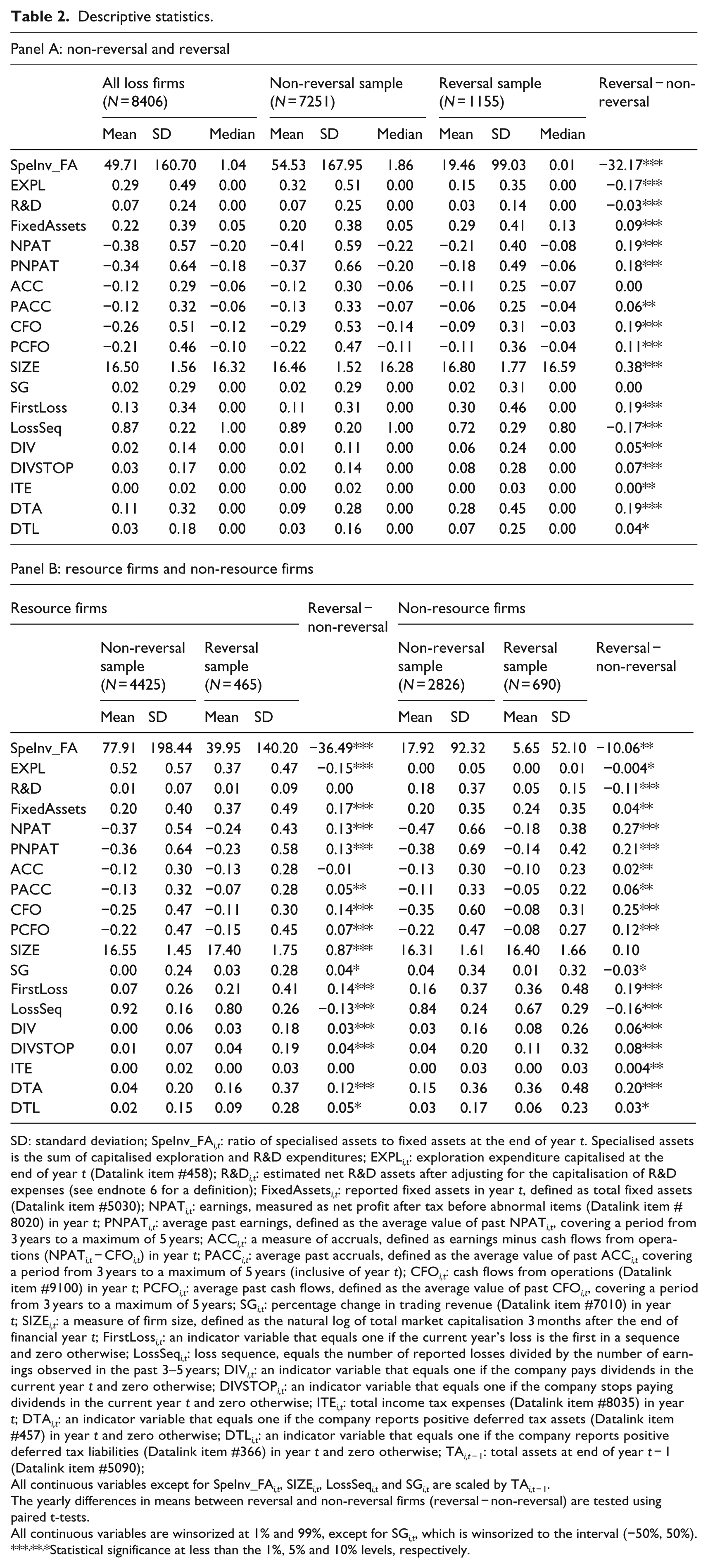
SD: standard deviation; SpeInv_FA _i,t : ratio of specialised assets to fixed assets at the end of year t. Specialised assets is the sum of capitalised exploration and R&D expenditures; EXPL _i,t : exploration expenditure capitalised at the end of year t (Datalink item #458); R&D _i,t : estimated net R&D assets after adjusting for the capitalisation of R&D expenses (see endnote 6 for a definition); FixedAssets _i,t : reported fixed assets in year t, defined as total fixed assets (Datalink item #5030); NPAT _i,t : earnings, measured as net profit after tax before abnormal items (Datalink item # 8020) in year t; PNPAT _i,t : average past earnings, defined as the average value of past NPAT _i,t , covering a period from 3 years to a maximum of 5 years; ACC _i,t : a measure of accruals, defined as earnings minus cash flows from operations (NPAT _i,t  − CFO _i,t ) in year t; PACC _i,t : average past accruals, defined as the average value of past ACC _i,t covering a period from 3 years to a maximum of 5 years (inclusive of year t); CFO _i,t : cash flows from operations (Datalink item #9100) in year t; PCFO _i,t : average past cash flows, defined as the average value of past CFO _i,t , covering a period from 3 years to a maximum of 5 years; SG _i,t : percentage change in trading revenue (Datalink item #7010) in year t; SIZE _i,t : a measure of firm size, defined as the natural log of total market capitalisation 3 months after the end of financial year t; FirstLoss _i,t : an indicator variable that equals one if the current year’s loss is the first in a sequence and zero otherwise; LossSeq _i,t : loss sequence, equals the number of reported losses divided by the number of earnings observed in the past 3–5 years; DIV _i,t : an indicator variable that equals one if the company pays dividends in the current year t and zero otherwise; DIVSTOP _i,t : an indicator variable that equals one if the company stops paying dividends in the current year t and zero otherwise; ITE _i,t : total income tax expenses (Datalink item #8035) in year t; DTA _i,t : an indicator variable that equals one if the company reports positive deferred tax assets (Datalink item #457) in year t and zero otherwise; DTL _i,t : an indicator variable that equals one if the company reports positive deferred tax liabilities (Datalink item #366) in year t and zero otherwise; TA_{i,t − 1}: total assets at end of year t − 1 (Datalink item #5090);

All continuous variables except for SpeInv_FA _i,t , SIZE _i,t , LossSeq _i,t and SG _i,t are scaled by TA_{i,t − 1}.

The yearly differences in means between reversal and non-reversal firms (reversal − non-reversal) are tested using paired t-tests.

All continuous variables are winsorized at 1% and 99%, except for SG _i,t , which is winsorized to the interval (−50%, 50%).

***,**,*Statistical significance at less than the 1%, 5% and 10% levels, respectively.

Panel A of Table 2 further shows that loss firms allocate a significant amount of resources to investment assets. The mean value of SpeInv_FA _i,t is large, at 49.71, compared with a median value of only 1.04. The sample contains observations with extremely large investments in specialised assets but a very low level of fixed-asset investment, consistent with the behaviour of firms in the early stage of investment. The mean value of EXPL _i,t is 0.29 per dollar of lagged total assets. The mean value of FixedAssets _i,t is 0.22. Consistent with Wu et al. (2010), panel A shows that Australian loss firms do not focus on R&D investment to the same extent as mineral exploration (mean R&D = 0.07). As expected, reversal firms have a significantly lower level of investment in specialised assets relative to fixed assets than non-reversal firms do (difference in mean SpeInv_FA _i,t  = −32.17). Reversal firms exhibit a significantly higher level of investment in fixed assets than non-reversal firms do (difference in mean FixedAssets _i,t  = 0.09). These results provide initial support for H1. In addition, reversal firms are generally larger (difference in mean SIZE _i,t  = 0.38), more likely to experience the first loss in a sequence (difference in mean FirstLoss _i,t  = 0.19), more likely to have a smaller number of past losses (difference in mean LossSeq _i,t  = −0.17) and more likely to have a generous dividend policy (difference in mean DIV _i,t  = 0.05). They also have higher income tax expenses, deferred tax assets and liabilities.

Panel B of Table 2 compares the reversal and non-reversal firms for the resource and non-resource subsamples separately. Reversal and non-reversal firms exhibit differences in investment activities in both subsamples. Reversal firms typically have smaller (larger) investments in specialised assets (fixed assets). The divergence in investment activities between reversal and non-reversal firms is stronger for the resource subsample, suggesting that investment activities are an important factor for assessing loss persistence for resource firms.

Table 3 presents the correlation matrix. The correlations among independent variables are mostly small, with the exception of the correlations between measures of loss patterns (FirstLoss _i,t and LossSeq _i,t ) and performance. It is evident that SpeInv_FA _i,t is significantly negatively correlated with 1-year-ahead loss reversal. The correlation between fixed assets and loss reversal is positive. Generally, the univariate analysis supports the predictions of H1.

OPEN IN VIEWER

Table 3.

Pearson (below the diagonal)/Spearman (above the diagonal) correlations.

	1	2	3	4	5	6	7	8	9	10	11	12	13	14	15	16	17	18	19	20
1. LossRev		−0.163	−0.132	0.006	0.134	0.225	0.220	−0.001	0.096	0.243	0.159	0.066	−0.011	0.195	−0.240	0.131	0.130	0.028	0.207	0.081
2. SpeInv_FA	−0.075		0.734	0.184	−0.521	−0.030	−0.148	0.093	−0.082	−0.107	−0.107	0.080	−0.052	−0.180	0.240	−0.116	−0.130	−0.032	−0.204	−0.023
3. EXPL	−0.118	0.336		−0.372	−0.253	0.076	−0.059	0.101	−0.041	0.007	−0.062	0.115	−0.034	−0.161	0.215	−0.104	−0.119	−0.003	−0.203	−0.019
4. R&D	−0.056	0.089	−0.163		0.030	−0.144	−0.082	−0.034	−0.046	−0.142	−0.040	0.102	0.028	0.024	−0.016	0.019	0.021	−0.047	0.071	0.025
5. FixedAssets	0.079	−0.165	−0.127	−0.043		0.029	0.128	−0.078	0.035	0.090	0.107	0.189	0.118	0.146	−0.169	0.117	0.118	−0.001	0.194	0.063
6. NPAT	0.121	0.026	−0.011	−0.232	−0.129		0.568	0.463	0.297	0.676	0.401	0.116	−0.037	0.285	−0.341	0.175	0.159	0.031	0.274	0.099
7. PNPAT	0.103	−0.017	−0.039	−0.120	−0.004	0.395		0.140	0.542	0.517	0.647	0.048	−0.093	0.420	−0.613	0.210	0.250	0.069	0.298	0.080
8. ACC	0.008	0.054	0.082	−0.007	−0.042	0.484	0.153		0.176	−0.199	0.065	0.026	−0.016	0.003	−0.006	0.000	−0.014	−0.052	0.010	−0.013
9. PACC	0.068	−0.038	−0.009	−0.130	−0.020	0.288	0.533	0.143		0.181	−0.090	−0.018	−0.011	0.200	−0.272	0.084	0.120	0.052	0.125	0.045
10. CFO	0.136	−0.004	−0.061	−0.259	−0.126	0.828	0.360	−0.019	0.241		0.415	0.094	−0.022	0.300	−0.369	0.171	0.178	0.075	0.273	0.125
11. PCFO	0.085	−0.005	−0.056	−0.055	0.015	0.285	0.747	0.099	−0.002	0.267		0.069	−0.081	0.279	−0.437	0.159	0.176	0.032	0.231	0.055
12. SG	0.076	−0.021	0.089	0.047	0.211	0.080	0.049	0.040	−0.012	0.063	0.071		0.080	0.063	−0.041	0.114	0.038	−0.017	0.149	0.136
13. SIZE	0.000	−0.037	−0.038	−0.008	0.116	−0.023	−0.043	−0.028	−0.014	−0.014	−0.044	0.075		−0.091	0.119	0.008	−0.035	−0.011	0.000	−0.013
14. FirstLoss	0.195	−0.073	−0.140	−0.057	0.061	0.151	0.182	0.028	0.131	0.156	0.139	0.076	−0.080		−0.591	0.264	0.333	0.014	0.320	0.124
15. LossSeq	−0.267	0.104	0.203	0.087	−0.084	−0.193	−0.277	−0.034	−0.182	−0.201	−0.230	−0.092	0.106	−0.658		−0.236	−0.281	−0.055	−0.355	−0.121
16. DIV	0.119	−0.042	−0.076	−0.031	0.070	0.074	0.081	0.012	0.041	0.074	0.075	0.131	0.014	0.240	−0.293		0.101	0.012	0.233	0.076
17. DIVSTOP	0.130	−0.053	−0.094	−0.034	0.047	0.083	0.107	0.007	0.078	0.090	0.086	0.051	−0.029	0.333	−0.366	−0.021		0.008	0.231	0.045
18. ITE	0.026	0.008	0.035	−0.124	−0.021	0.055	0.056	−0.061	0.060	0.106	0.026	−0.015	−0.003	0.018	−0.050	0.023	0.030		−0.092	−0.067
19. DTA	0.207	−0.087	−0.168	−0.036	0.107	0.142	0.125	0.042	0.073	0.136	0.110	0.171	0.010	0.320	−0.419	0.207	0.231	−0.093		0.220
20. DTL	0.081	0.008	−0.036	−0.014	0.041	0.067	0.045	0.007	0.007	0.072	0.048	0.158	−0.026	0.124	−0.147	−0.018	0.045	−0.040	0.220

The variables are defined in Table 2.

All continuous variables are winsorized at 1% and 99%, except for SG _i,t , which is winsorized to the interval (−50%, 50%).

Significant correlations are in bold (at the 5% level).

6. Results

6.1. Predicting loss reversal

Four specifications of the loss reversal model are used to examine factors associated with a 1-year-ahead loss reversal. Specifications I and II are the original JP models extended by including the three tax variables. Specification I measures the firms’ current and past performance using earnings (NPAT _i,t and PNPAT _i,t ), ¹³ while Specification II uses accruals (ACC _i,t and PACC _i,t ) and cash flows (CFO _i,t and PCFO _i,t ) as specified in equation (1). Specification III is equation (1), which includes the ratio of specialised investment to fixed assets (SpeInv_FA _i,t ). Hypothesis H1 is examined using this specification. The last specification (IV) replaces SpeInv_FA _i,t with exploration investment (EXPL _i,t ), R&D investment (R&D _i,t ) and fixed-asset investment (FixedAssets _i,t ). Following Joos and Plesko (2005), all models are estimated as logistic regressions using the Fama and MacBeth (1973) procedures. The results are presented in Table 4, panel A.

OPEN IN VIEWER

Table 4.

Results for predicting loss reversal.

Panel A: results for logistic loss-reversal models
	Pred.	One-year-ahead loss reversal				Three-year-ahead loss reversal
		Specification I	Specification II	Specification III	Specification IV	Specification III
SpeInv_FA (t-stat)	−			−0.007*** (−4.182)		−0.002*** (−4.752)
EXPL	−				−0.819*** (−3.581)
R&D	−				−0.435 (−0.696)
FixedAssets	+				0.422***   (3.674)
NPAT	+	0.932*** (5.596)
PNPAT	+	0.446** (2.278)
ACC	+		0.548*** (3.051)	0.616***    (3.742)	0.770*** (3.776)	0.255**  (2.157)
PACC	+		0.127 (0.693)	0.125 (0.712)	0.098 (0.543)	0.099 (0.726)
CFO	+		1.716*** (6.142)	1.701*** (6.438)	1.817*** (6.027)	0.770*** (3.849)
PCFO	+		0.326 (1.401)	0.327 (1.329)	0.354 (1.283)	0.174**  (2.194)
SIZE	+	−0.005 (−0.482)	−0.007 (−0.568)	−0.007 (−0.577)	−0.005 (−0.449)	0.040*** (4.812)
SG	+	0.476** (2.415)	0.448**   (2.190)	0.398* (1.990)	0.319 (1.597)	0.409*** (4.162)
FirstLoss	+	−0.057 (−0.313)	−0.063 (−0.345)	−0.075 (−0.417)	−0.115 (−0.632)	0.150 (1.283)
LossSeq	−	−1.962*** (−8.874)	−1.900*** (−8.44)	−1.744*** (−7.538)	−1.789*** (−8.340)	−1.694*** (−9.720)
DIV	+	4.142 (0.653)	4.403 (0.777)	4.137 (0.756)	4.283 (0.807)	10.014 (1.054)
DIVSTOP	−	0.176 (0.921)	0.145 (0.783)	0.147 (0.804)	0.079 (0.437)	0.084 (0.361)
ITE	+	5.166** (2.219)	3.749 (1.377)	3.720 (1.426)	4.135 (1.550)	2.203 (0.744)
DTA	+	0.559*** (4.128)	0.521*** (3.923)	0.466*** (3.505)	0.400*** (3.028)	0.723*** (7.682)
DTL	+	0.048 (1.268)	0.032 (1.032)	0.031 (0.914)	0.014 (0.409)	0.071 (0.872)
Ave. LR p value		<0.0001	<0.0001	<0.0001	<0.0001	<0.0001
Ave. % concordant		74.78%	75.76%	77.12%	77.76%	71.86%
N		8406	8406	8406	8406	8406

Panel B: fitted value of reversal probabilities
		Non-reversal sample (N = 7251)	Loss-reversal sample (N = 1155)	Difference in yearly means (t-stat)
Specification I	Mean (median) [SD]	0.119 (0.091) [0.105]	0.261 (0.192) [0.196]	0.133*** (16.764)
Specification II	Mean (Median) [SD]	0.117 (0.089) [0.108]	0.270 (0.203) [0.200]	0.144*** (16.709)
Specification III	Mean (Median) [SD]	0.115 (0.086) [0.111]	0.277 (0.217) [0.197]	0.152*** (16.461)
Specification IV	Mean (Median) [SD]	0.114 (0.081) [0.114]	0.288 (0.228) [0.205]	0.164*** (15.335)

Panel C: out-of-sample classification accuracy (specification III)
Rank of predicted likelihood of loss reversal	Non-reversal sample	Loss-reversal sample	Total
1 Predicted persistent losses (column percentage)	1914 (27.19%)	113 (10.36%)	2027
2	1871 (26.58%)	164 (15.03%)	2035
3	1788 (25.40%)	250 (22.91%)	2038
4 Predicted transitory losses	1466 (20.83%)	564 (51.70%)	2030
Total	7039	1091	8130

Panel D: Type I and Type II errors for selected cut-off points (specification III)
Top X percentile of predicted probability of loss reversal as the cut-off point (%)	Type I errors (%)	Type II errors (%)
90	89.16	3.94
75	72.81	10.36
67	63.79	14.21
50	46.23	25.39
33	29.12	39.60
25	20.83	48.30
10	7.20	72.50

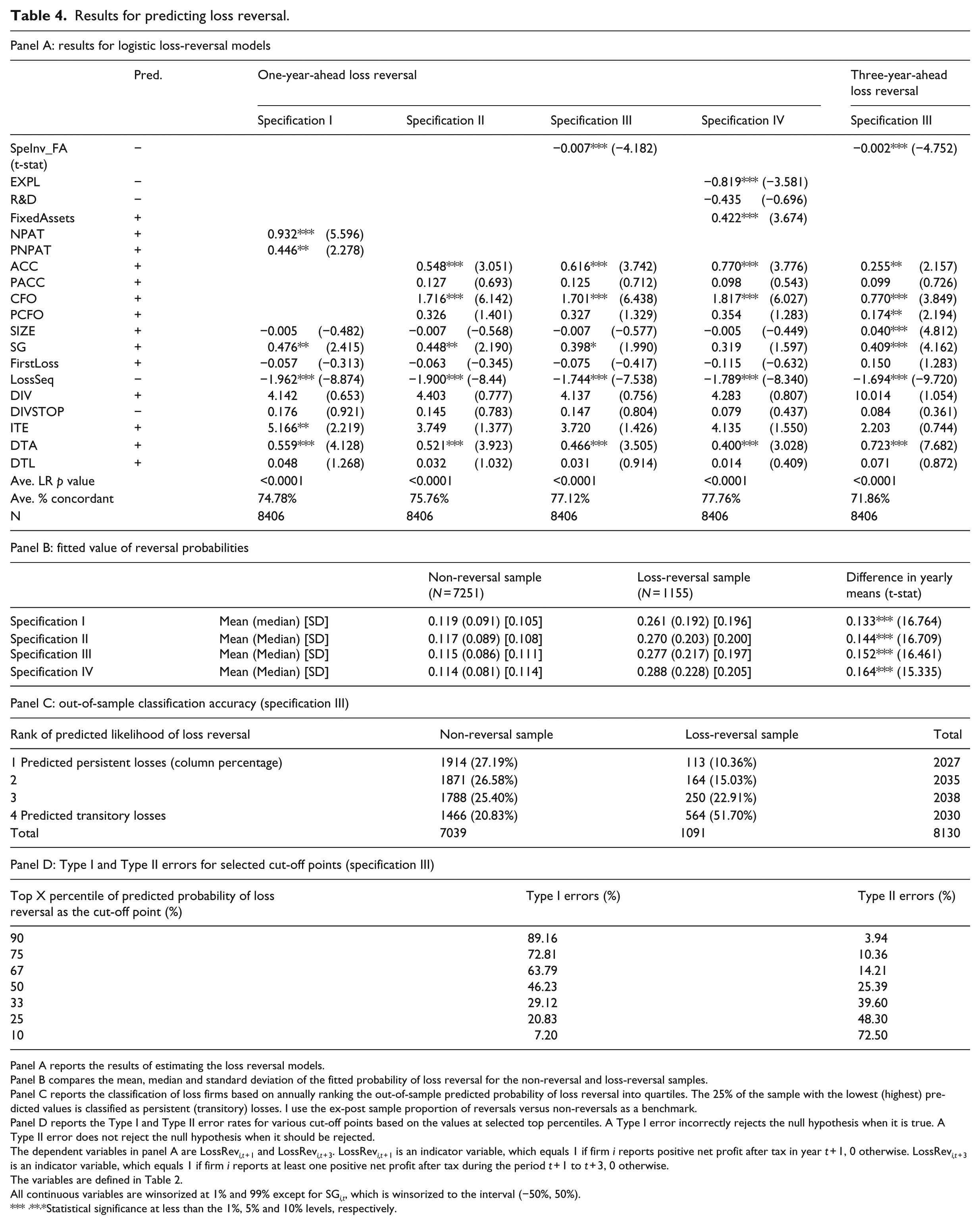
Panel A reports the results of estimating the loss reversal models.

Panel B compares the mean, median and standard deviation of the fitted probability of loss reversal for the non-reversal and loss-reversal samples.

Panel C reports the classification of loss firms based on annually ranking the out-of-sample predicted probability of loss reversal into quartiles. The 25% of the sample with the lowest (highest) predicted values is classified as persistent (transitory) losses. I use the ex-post sample proportion of reversals versus non-reversals as a benchmark.

Panel D reports the Type I and Type II error rates for various cut-off points based on the values at selected top percentiles. A Type I error incorrectly rejects the null hypothesis when it is true. A Type II error does not reject the null hypothesis when it should be rejected.

The dependent variables in panel A are LossRev_i,t + 1 and LossRev_i,t + 3. LossRev_i,t + 1 is an indicator variable, which equals 1 if firm i reports positive net profit after tax in year t + 1, 0 otherwise. LossRev_i,t + 3 is an indicator variable, which equals 1 if firm i reports at least one positive net profit after tax during the period t + 1 to t + 3, 0 otherwise.

The variables are defined in Table 2.

All continuous variables are winsorized at 1% and 99% except for SG _i,t , which is winsorized to the interval (−50%, 50%).

***,**,*Statistical significance at less than the 1%, 5% and 10% levels, respectively.

The results for specification III show that the coefficient of SpeInv_FA _i,t is significantly negative (−0.007, t-stat = −4.182), consistent with the prediction of H1. Firms with a higher level of specialised investment relative to fixed-asset investment are more likely to face persistent losses. The results for specification IV further show that exploration assets are significantly negatively associated with future loss reversal (EXPL _i,t  = −0.819, t-stat = −3.581). In contrast, the level of investment in fixed assets is associated with a higher likelihood of loss reversal (FixedAssets _i,t  = 0.422, t-stat = 3.674). ¹⁴ Together, these findings suggest that, while a high level of investment in specialised assets indicates persistent losses, firms that invest heavily in fixed assets are more likely to become profitable.

Consistent with the prior literature, across all four specifications, the coefficients of measures of performance (NPAT _i,t , ACC _i,t and CFO _i,t ), loss pattern (LossSeq _i,t ), dividend payments (DIV _i,t ) and reported tax items (ITE _i,t and DTA _i,t ) are significant, with the predicted signs. The within-sample performances of all four specifications are quite similar. The average p values for the likelihood ratio are less than 0.0001. The average percentage concordant pair classification increases from 74.78% for specification I to 77.76% for specification IV. This result is comparable with prior US studies, ¹⁵ indicating that the JP model and its various extensions produce reasonable explanations for loss reversal in Australia.

The final column of panel A in Table 4 reports the results from using specification III to explain 3-year-ahead loss reversal. ¹⁶ The results show that the relation between SpeInv_FA _i,t and loss reversal remains significantly negative (−0.002, t-stat = −4.752). This finding confirms the prediction of H1. Other factors, including accruals, cash flows, firm size, sales growth and deferred tax assets, are also found to be associated with 3-year-ahead loss reversal.

A simple within-sample evaluation of the loss-reversal models is performed. Panel B of Table 4 presents the average fitted values for the non-reversal sample and the loss-reversal sample. It shows that the mean fitted probability of loss reversal for the non-reversal sample ranges from 0.119, using specification I, to 0.114, using specification IV. In contrast, the average fitted value for the loss-reversal sample is more than two times higher than for the non-reversal firms, ranging from 0.261, using specification I, to 0.288, using specification IV. For all specifications, the differences in the yearly average fitted probability of loss reversal between reversal and non-reversal firms are statistically significant.

To examine the predictive power of equation (1), I calculate an out-of-sample ex-ante probability of loss reversal following the procedures described in the research design section. ¹⁷ This reduces the sample size to 8130. I compare the distributions of sample quartiles between the actual loss-reversal and non-reversal samples. Panel C of Table 4 reports the results, which show that 51.7% of observations that experience subsequent loss reversal fall in the top quartile (transitory-loss sample). Another 22.91% of reversal firms fall in the second-highest ranked quartile. In contrast, only 10.36% of reversal firms are incorrectly classified as persistent-loss firms in the bottom quartile. ¹⁸

Panel D of Table 4 reports the frequencies of Type I and Type II errors for the out-of-sample prediction. In this case, a Type I error occurs when a non-reversal firm is incorrectly predicted to reverse. In contrast, a Type II error occurs when a reversal firm is incorrectly classified as a non-reversal. I report the predictive performance of the model at various cut-off points. As shown, there is an obvious trade-off between Type I and Type II errors. As the cut-off point moves from the value at the 90th percentile (i.e. the top 90% of firms are classified as reversal firms) to the 10th percentile value, the Type I error rate declines, while the Type II error rate increases. Both types of error are below 50% when the cut-off point is set between the 50th and 25th percentiles, suggesting that the loss reversal model performs better within this range. ¹⁹

6.2. Future stock performance and the predicted probability of loss reversal

This section examines H2, which relates the predicted probability of loss reversal to future abnormal returns (BHAR_i,t + 1). Recall that both a portfolio method and a regression method are used to test H2. ²⁰ Panel A of Table 5 reports the mean BHAR_i,t + 1 for the four portfolios formed at the level of the predicted likelihood of loss reversal. It also reports the mean BHAR_i,t + 1 of the zero-investment hedge portfolios. The results show that, as the predicted probability of loss reversal increases from the persistent-loss portfolio to the transitory-loss portfolio, BHAR_i,t + 1 becomes less negative. For example, the mean value-weighted BHAR_i,t + 1 values are −0.293 and −0.081 for the persistent-loss portfolio and the transitory-loss portfolio, respectively. The changes are mostly monotonic. The results for the equal-weighted BHAR_i,t + 1 are similar. On average, value-weighted hedge portfolios generate an average annual BHAR_i,t + 1 of 21.2% (12.9% for equal-weighted hedge portfolios). ²¹ Overall, future abnormal returns increase with the predicted probability of loss reversal. It is also interesting to observe that abnormal returns are significantly negative for all four portfolios. This result indicates that investors may overestimate the probability of loss reversal for even the transitory-loss group. This conclusion is consistent with the results reported by Li (2011).

OPEN IN VIEWER

Table 5.

Future stock performance and the predicted probability of loss reversal.

Panel A: future BHARs for portfolios sorted by the predicted probability of loss reversal
Portfolio ranking	Value-weighted BHAR	Equal-weighted BHAR
1 Predicted persistent loss (t-stat)	−0.293*** (−6.745)	−0.284*** (−7.564)
2	−0.247*** (−4.081)	−0.142* (−1.856)
3	−0.178** (−3.774)	−0.200*** (−6.089)
4 Predicted transitory loss	−0.081** (−2.203)	−0.155*** (−4.666)
Hedge portfolio (transitory–persistent)	0.212**   (3.858)	0.129***   (2.941)

Panel B: future abnormal returns on the probability of loss reversal
	All firms		No analyst following	With analyst following	Non-ASX200	ASX200
Rplorev (t-stat)	0.038*** (5.85)	0.025*** (3.18)	0.025*** (3.07)	0.004 (0.14)	0.025*** (3.19)	−0.006 (−0.19)
NPAT		0.051*** (2.65)	0.043** (2.22)	0.180 (1.54)	0.041** (2.23)	0.036   (0.30)
ACC		−0.072** (−2.20)	−0.069** (−2.10)	−0.113 (−0.63)	−0.056* (−1.78)	−0.233 (−1.12)
VOL		−0.246*** (−3.89)	−0.239*** (−3.62)	−0.162 (−0.59)	−0.204*** (−3.21)	−0.236 (−0.79)
DIV		0.061 (1.42)	0.032 (0.55)	0.080 (1.17)	0.089* (1.61)	−0.102 (−1.36)
ZScore		−0.001** (−2.82)	−0.001*** (−2.88)	0.000 (0.32)	−0.001*** (−2.66)	−0.001* (−1.95)
Intercept	−0.267*** (−21.77)	−0.172*** (−7.71)	−0.179*** (−7.69)	−0.098 (−1.10)	−0.209*** (−9.58)	0.068 (0.67)
N	6470	6470	5766	704	5696	774
R 2	0.4%	1.0%	1.0%	1.1%	1.0%	0.6%

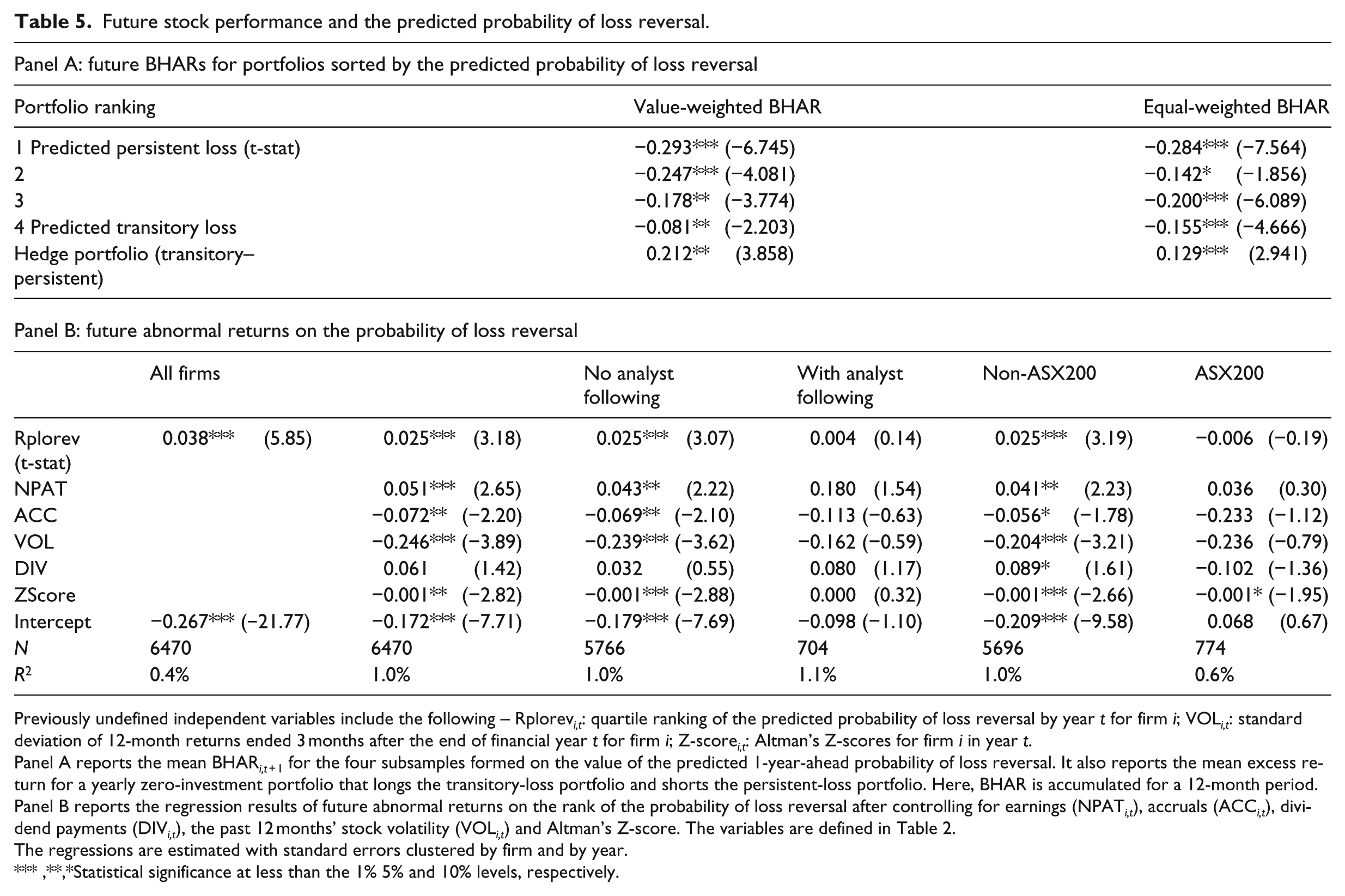
Previously undefined independent variables include the following – Rplorev _i,t : quartile ranking of the predicted probability of loss reversal by year t for firm i; VOL _i,t : standard deviation of 12-month returns ended 3 months after the end of financial year t for firm i; Z-score _i,t : Altman’s Z-scores for firm i in year t.

Panel A reports the mean BHAR_i,t + 1 for the four subsamples formed on the value of the predicted 1-year-ahead probability of loss reversal. It also reports the mean excess return for a yearly zero-investment portfolio that longs the transitory-loss portfolio and shorts the persistent-loss portfolio. Here, BHAR is accumulated for a 12-month period.

Panel B reports the regression results of future abnormal returns on the rank of the probability of loss reversal after controlling for earnings (NPAT _i,t ), accruals (ACC _i,t ), dividend payments (DIV _i,t ), the past 12 months’ stock volatility (VOL _i,t ) and Altman’s Z-score. The variables are defined in Table 2.

The regressions are estimated with standard errors clustered by firm and by year.

***,**,*Statistical significance at less than the 1% 5% and 10% levels, respectively.

The results of the regression method are reported in Table 5, panel B. The first two columns report the regression results for the full sample. Two models are used. The first model regresses BHAR_i,t + 1 on the ranked value of the predicted probability of loss reversal (Rplorev _i,t ) only, ²² while the second model is equation (2). The results show that the coefficient of Rplorev _i,t is significantly positive (for equation (2), the coefficient is 0.025, with t-stat = 3.18). This indicates that future abnormal returns are higher for firms with a higher predicted probability of future loss reversal. While abnormal returns are negatively associated with bankruptcy risk, it does not appear that Rplorev _i,t and ZScore _i,t capture similar effects. ²³ The adjusted R² value is 1.0% for equation (2). Other control variables, except for dividends, are also significant.

The results reported thus far show that future abnormal returns are associated with the predicted probability of loss reversal for loss firms. Prior literature, however, suggests that this result may be conditional on loss firms’ information environment (Dhaliwal et al., 2013). Investors in loss firms with a better information environment are less likely to misunderstand the signals contained in accounting information for future profitability. I further investigate this proposition. The information environment is measured by analyst coverage and security index inclusion (ASX 200), both of which suggest better visibility and an improved information environment. ²⁴ I estimate equation (2) for firms with/without analyst following, as well as ASX 200/non-ASX 200 firms. ²⁵ The results are reported in the last four columns of panel B, Table 5. It is shown that the positive association between the probability of loss reversal and future abnormal returns is observed only for loss firms not followed by analysts or not included in the ASX 200 index. This result demonstrates that improvement in loss firms’ information environment helps investors better process accounting information.

6.3. Probability of loss reversal for resource and non-resource firms

This section applies the loss-reversal model to resource and non-resource firms separately. The analysis has two motivations: first, the large presence of resource-based loss firms in the Australian market and, second, the concern that the results may be driven by the difference between resource and non-resource loss firms. Table 1 shows that the percentage of loss reversal for resource firms is smaller than other firms. The association between SpeInv_FA _i,t and future loss reversal may simply reflect the difference in the probability of loss reversal between resource firms and other firms.

Panel A of Table 6 reports the results of estimating equation (1) for the two subsamples. As reported in Table 1, the resource-based subsample includes 4890 firm-year observations, while the non-resource subsample has 3516 observations. Consistent with the prediction of H1, the coefficient of SpeInv_FA _i,t is significantly negative (−0.005) at less than the 1% level for resource-based loss firms. This suggests that higher expenditures on specialised assets (mainly exploration investment) relative to fixed assets indicate a lower likelihood of loss reversal in the following period. In addition, measures of performance, including ACC _i,t and CFO _i,t , are positively associated with loss reversal, while LossSeq _i,t is negatively associated with loss reversal. Panel B further shows that out-of-sample predictions classify 63.82% (43.82%) of resource firms with actual loss reversal into the top two (top) quartiles.

OPEN IN VIEWER

Table 6.

Predicting loss reversal for resource firms and non-resource firms.

Panel A: results for logistic loss-reversal models (specification III)
	Pred.	Resource firms	Non-resource firms
SpeInv_FA (t-stat)	−	−0.005*** (−3.735)	−0.040   (−1.505)
ACC	+	0.879* (1.723)	2.225*** (3.100)
PACC	+	1.271 (1.629)	−0.109 (−0.232)
CFO	+	1.959*** (3.743)	4.008*** (4.115)
PCFO	+	1.294* (1.838)	0.562 (1.54)
SIZE	+	0.010 (0.589)	0.001 (0.057)
SG	+	0.936** (2.334)	−0.026 (−0.118)
FirstLoss	+	−0.287 (−1.215)	0.022 (0.098)
LossSeq	−	−2.369*** (−5.962)	−1.13*** (−4.816)
DIV	+	17.635 (0.833)	8.617 (0.999)
DIVSTOP	−	1.658 (0.697)	−0.068 (−0.253)
ITE	+	4.833 (1.074)	−3.933 (−0.436)
DTA	+	−1.720 (−1.341)	0.174 (0.957)
DTL	+	0.159 (1.684)	−0.04 (−1.337)
Average LR p value		<0.0001	<0.0001
Average % concordant		78.50%	79.79%
N		4890	3516

Panel B: out-of-sample classification accuracy
Rank of predicted likelihood of loss reversal	Resource firms		Non-resource firms
	Non-reversal sample	Loss-reversal sample	Non-reversal sample	Loss-reversal sample
1 Predicted persistent losses	1094	79	788	55
(column percentage)	25.58%	17.75%	28.52%	8.51%
2	1102	82	740	116
	25.77%	18.43%	26.78%	17.96%
3	1098	89	685	173
	25.68%	20.00%	24.79%	26.78%
4 Predicted transitory losses	982	195	550	302
	22.97%	43.82%	19.91%	46.75%
Total	4276	445	2763	646

Panel C: future value-weighted BHARs for portfolios sorted by the predicted probability of loss reversal for resource firms and non-resource firms
Portfolio ranking	Resource firms value-weighted BHAR	Non-resource firms value-weighted BHAR
1 Predicted persistent loss (t-stat)	−0.203** (−4.144)	−0.440*** (−8.935)
2	−0.202*** (−2.968)	−0.210** (−2.253)
3	−0.253*** (−6.526)	−0.154** (−2.363)
4 Predicted transitory loss	−0.074 (−1.383)	−0.163*** (−4.101)
Hedge portfolio (transitory–persistent)	0.129** (2.487)	0.280** (5.111)

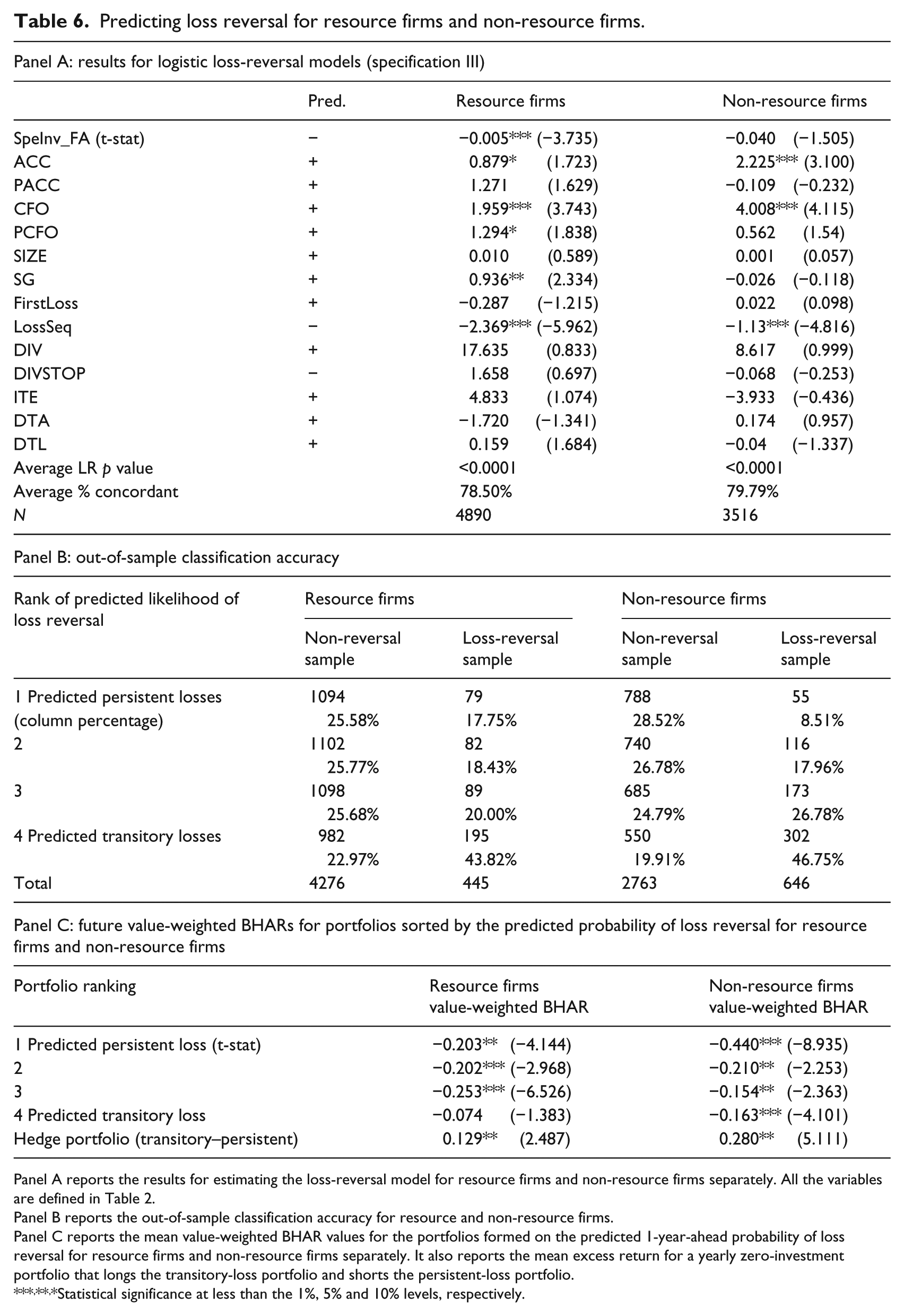
Panel A reports the results for estimating the loss-reversal model for resource firms and non-resource firms separately. All the variables are defined in Table 2.

Panel B reports the out-of-sample classification accuracy for resource and non-resource firms.

Panel C reports the mean value-weighted BHAR values for the portfolios formed on the predicted 1-year-ahead probability of loss reversal for resource firms and non-resource firms separately. It also reports the mean excess return for a yearly zero-investment portfolio that longs the transitory-loss portfolio and shorts the persistent-loss portfolio.

***,**,*Statistical significance at less than the 1%, 5% and 10% levels, respectively.

The regression results for the non-resource sample are presented in the final column of panel A of Table 6. Contrary to the prediction of H1, the association between SpeInv_FA _i,t and future loss reversal is negative but insignificant (−0.040, t-stat = −1.505). However, untabulated results report a significantly positive coefficient for FixedAssets _i,t . This suggests that a higher level of fixed assets indicates a higher probability of future loss reversal. As shown in panel B, 73.53% (46.75%) of loss-reversal firms are correctly classified into the highest two (top) quartiles of the predicted probability of loss reversal. In summary, there are notable differences in predicting loss reversal for resource and non-resource-based firms. This suggests a need for developing more industry-specific loss-reversal models.

Lastly, I conduct the portfolio test for the resource and non-resource subsamples. Panel C of Table 6 reports these results for value-weighted portfolios. ²⁶ The results show that, for resource firms, the average abnormal return for transitory-loss portfolios is less negative (BHAR_i,t + 1 = −0.074) than for persistent-loss portfolios (BHAR_i,t + 1 = −0.203). The hedge portfolios of resource firms generate a significant mean value-weighted annual abnormal return of 12.9% before transaction costs. Similarly, hedge portfolios for non-resource firms, on average, generate a significant annual abnormal return of 28%. This result suggests that investors may not correctly assess the probability of loss reversal for either resource or non-resource loss firms.

7. Conclusion

Investors in loss firms make abandonment decisions based on their assessment of the probability of future loss reversal. This research examines factors associated with the likelihood of future loss reversal for Australian loss firms. It further examines how investors incorporate the implications of these future-performance factors in the valuation.

The results suggest that, apart from the known factors examined in the US literature, investment activities can also be indicative of future loss reversal. Loss firms engaging in specialised investment, such as mineral exploration and R&D, are more likely to experience persistent losses. When loss firms move closer to the commercial stage, as indicated by higher investment in long-term fixed assets, they are more likely to become profitable. Investors appear to underestimate the persistence of losses for firms with a weak information environment. Subsequent realisation of the persistence of losses causes significant negative returns.

This research has several implications. First, investors can adopt a set of financial variables to assess the likelihood of future loss reversal in Australia. These factors cover loss firms’ past performance, loss patterns, dividend payments and reported tax items. Second, given the high incidence of loss firms that are investment intensive (Darrough and Ye, 2007; Wu et al., 2010), loss firms’ investment activities may be informative in assessing the likelihood of future loss reversal. Third, the persistence of losses may be higher than the level typically anticipated by the market. Investors should consider lowering their expectations and demand more information from loss firms and financial analysts.

Given the prevalence and diversity of loss firms in the Australian market, future research can expand the set of factors used in predicting future loss reversal. The current research examines the probability of loss reversal for up to three future years. Future research could investigate the probability of loss reversal in a longer timeframe. This article also finds evidence suggesting that the performance of the loss-reversal model differs across industries. This calls for the development of industry-specific loss-reversal models in future studies.