Comparative Appraisal of Critical Gap Estimation Techniques in the Context of U-turning Vehicles

Abstract

Critical gap is a crucial factor for capacity estimation and safety evaluation at uncontrolled mid-block median openings (MBMOs). The U-turning vehicle makes a U-turn when a sufficient gap between two fast-moving vehicles is available in the approaching through traffic (ATT) stream. Even though, worldwide, temporal gaps are extensively used, the spatial gap is an important parameter that significantly affects minor street vehicles’ safety (U-turning vehicles in this study). The present research, undertaken in India, focuses on estimating the temporal and spatial critical gap of U-turning vehicles at uncontrolled MBMOs. The collected data were analyzed for six different types of U-turning vehicles at varying approaching through traffic volume (ATTV). For critical gap estimation, four different critical gap estimation techniques, namely, modified Raff method (MRM), Ashworth method, binary logit model (BLM) method, and occupancy time (OT) method were employed, separately. From the analysis, temporal and spatial critical gaps were observed to vary between different types of vehicle, and it was also observed to vary with ATTV. The critical gap values of this study were found to be smaller than the critical values reported in developed countries, signifying the aggressive driving nature of drivers in developing countries. A detailed appraisal of the different critical gap estimation methods has been carried out. From this analysis, the OT method was found to provide the closest critical gap values with the published literature compared with other methods. Lastly, the findings from the present study will be useful for capacity estimation and safety evaluation at MBMO.

Keywords

data and data science statistical methods analysis modeling operations traffic flow theory and characteristics traffic flow

Gap acceptance behavior is an important phenomenon that affects the performance and safety of an unsignalized intersection. Mid-block median openings (MBMOs) are a peculiar type of intersection that operate similarly to unsignalized intersections based on the perception of minor and major street vehicle drivers ( 1 – 3 ). Although the traffic operation at MBMOs is similar to unsignalized intersections, the complexity associated with the U-turning vehicle gap acceptance is greater ( 4 , 5 ).

MBMOs are provided in the raised median to vehicles to make a U-turn and reverse their flow direction ( 6 ). A U-turn maneuver is possible only if the desired gap of the U-turning driver is available in approaching through traffic (ATT) stream. If the desired gap is not available, then the U-turning vehicle faces delay. Delay faced by U-turning vehicles depends on many factors, such as approaching through traffic volume (ATTV), U-turning driving behavior, and other operating conditions ( 2 , 7 ). If a U-turning vehicle driver has aggressive driving behavior, they accept a shorter gap and face less delay, but create a risky situation and increase the likelihood of collision at the MBMO. Generally, in developed countries such as the United States and Canada, these uncontrolled MBMOs are controlled by stop or yield signs for giving priority to various movements. ( 8 – 10 ). But in India, different types of vehicles (two-wheelers [2W], three-wheelers [3W], cars, buses, slow-moving vehicles, and pedestrians) use the same road section simultaneously without any physical separation. Therefore, the traffic condition in India is termed heterogeneous. Moreover, at most of the unsignalized intersection, stop and yield signs are not provided. Even if priority movement is specified with proper stop and yield signboards, drivers habitually violate the priority ( 2 , 11 , 12 ).

At MBMOs, when a U-turning vehicle waits to take a U-turn to merge with the ATT, the U-turning vehicle is presented with several gaps between two consecutive approaching through vehicles. Consequently, the U-turning vehicle driver assesses the size of the available gap and decides whether to accept the available gap or reject it. When a sufficient gap between two approaching through vehicles is available, only then does the U-turning vehicle start moving into the MBMO area and merge with the ATT. Additionally, both U-turning traffic and ATT are heterogeneous in nature.

Ashworth and Green defined the gap and described it as the difference in time between the back bumper of the lead vehicle and the front bumper of the following vehicle crossing the reference point in the ATT stream ( 13 ). The researchers adopt the term “critical gap” to represent the minimum size of the gap which a vehicle in the minor stream accepts to complete the merging or crossing. Likewise, U-turning vehicles’ critical gap can be defined as the minimum gap accepted by U-turning vehicles for completing the U-turn. The critical gap is an important factor for understanding the gap acceptance behavior of drivers at unsignalized intersections. Moreover, it is beneficial in the capacity estimation, level of service (LOS), and safety analysis at these facilities ( 14 , 15 ). Likewise, the critical gap values estimated using different methods have been utilized by various researchers for the estimation of U-turn capacity and LOS analysis at MBMO areas ( 16 , 17 ).

Motivations of the Study

The research on critical gap analysis dates back to the 1950s, and one of the earliest studies on critical gaps was carried out by Raff and Hart ( 18 ). The authors defined the critical gap as the gap for which the number of accepted gaps shorter than critical gap and the number of rejected gaps longer than critical gap is equal. Velan and Van Aerde termed the sum of decision time, maneuvering time, clearing time, and buffer time for safety as the critical gap ( 19 ). Greenshield defined critical gap as the gap range that has equal numbers of acceptance and rejection. In the 1985 and 2000 Highway Capacity Manual (HCM), the term critical gap was used, but the 2010 HCM used critical headway without differentiating it from the critical gap ( 20 – 22 ). HCM 2010 defines critical gap (critical headway) as the minimum time interval between two vehicles in conflicting traffic streams accepted by a minor street vehicle to complete the maneuver ( 22 ). It is a known fact that critical gap cannot be measured in the field directly—it has to be calculated mathematically by various deterministic, probabilistic approaches by collecting accepted and rejected gaps ( 1 , 11 , 23 –27). Furthermore, it is also known that the value of critical gap varies between different categories of vehicle, road geometry, driver behavior and age, and traffic conditions ( 5 ).

Most of the published articles on critical gap estimation have been developed under homogeneous traffic conditions where the ATT stream enjoys uninterrupted flow, and the rule of priority is always followed. Different researchers have adopted varying statistical techniques to compute the critical gaps at uncontrolled intersections ( 23 , 28 –30). The traffic condition of uninterrupted flow of ATT and priority movement rule is followed in developed countries, but in India and other developing world countries the rule of priority is often violated. Moreover, the traffic flow at uncontrolled intersections operates solely on user perceptions ( 31 ). Additionally, at uncontrolled intersections, the minor road vehicles are frequently observed to enter the intersection area forcefully and modify the natural traffic flow, resulting in safety concerns ( 32 , 33 ).

The established critical gap estimation methods have been developed by researchers working in developed countries having homogenous, lane-disciplined traffic. But, as mentioned earlier, the gap acceptance phenomenon is utterly different in developing countries. Therefore, a simple yet realistic method utilizing occupancy time (OT) has been employed for critical gap estimation in this study. OT is defined as the time between the arrival of the front bumper of a vehicle in the conflicting area and the departure of the rear bumper from the conflicting area. Additionally, the critical advantage of this method is that it can estimate the critical cap correctly at both homogeneous and heterogeneous traffic conditions ( 34 ). It can also estimate the critical gap precisely at locations where vehicles try to accept gaps while moving in a zig-zag style, and this kind of movement is very common in non-lane-disciplined traffic conditions ( 32 ). Zig-zag style refers to movement carried out in a haphazard or disorganized manner (35, 36). Zig-zag style movement is generally observed for 2W drivers. 2W drivers habitually explore every available gap and try to squeeze between bigger size vehicles utilizing small gaps ( 9 ). This type of driving behavior is common in heterogeneous traffic conditions ( 5 , 34 ).

The spatial gap is an important parameter and significantly affects the safety of minor stream traffic because in real-world conditions a road user intending to do a crossing or merging maneuver generally decides about the maneuver based on the distance available rather than the time gap ( 11 , 15 , 37 ). None of the studies tried to explore U-turning vehicles’ spatial critical gap, to the best of the authors’ knowledge. Moreover, various new statistical techniques, like the binary logit model (BLM) method, have the robustness to deal with the wide variability and nonlinearity in accepted and rejected gap data ( 37 ). Furthermore, the critical gap varies with varying ATTV. An in-depth study of the gap acceptance phenomenon with varying ATTV for different categories of vehicles with various new and traditional estimation techniques is needed to appraise critical gap estimation techniques’ suitability for varying operating conditions.

In the premise of the above-mentioned research gaps, the present study is carried out with the following objectives:

To estimate the critical gap for different types of U-turning vehicles at MBMOs at varying ATTV based on the OT and BLM method, and comparing the obtained results with different established methods like MRM and the Ashworth method.

To analyze the effect of varying ATTV on the estimated critical gaps of different types of vehicle as the change in ATTV changes the gap acceptance phenomenon at the MBMO area.

To compute the spatial critical gap of different vehicles at varying ATTV.

Critical Gap Estimation Methods

The critical gap is one of the most crucial parameters to understand minor road vehicles’ gap acceptance behavior. As the critical gap could not be directly measured in the field, several statistical techniques have been employed by various researchers to estimate the realistic critical gap ( 1 , 11 , 29 ). Furthermore, critical gap differs for different types of vehicles (2W, 3W, cars, buses, trucks, etc.), different traffic condition (homogeneous and heterogeneous), the geometry of road (6-lane and 4-lane), different driver characteristics such as driver age, driver experience, driver gender, and so forth, and, therefore, it is not feasible to measure critical gap for individual drivers ( 29 , 38 , 39 ). Likewise, a particular estimation technique is not suitable for the estimation of critical gap in different traffic scenarios. Therefore, this study is undertaken to estimate the critical gap of vehicles taking U-turns with different methods. The critical gap is defined as the minimum gap required by the U-turning vehicle to complete the U-turn without collision and merge with the ATT. The critical gap is a parameter that varies because of the geometry of intersections, different drivers, and various operational parameters. Other authors have developed various models and presented multiple critical gap estimation methods because of the reason mentioned above. Most of the methods are developed in homogeneous traffic conditions. In contrast, very few studies have been carried out to develop a robust method having applicability of critical gap estimation in homogeneous and heterogeneous traffic conditions. Mohan and Chandra have developed a new concept for critical gap estimation which provides reasonable results in both homogeneous and heterogeneous traffic conditions ( 34 ). In the present study, four different methods have been used for the estimation of the critical cap. All the different methods have been explained briefly in the sub-sections below.

Modified Raff Method (MRM)

The very first method was introduced by Raff and Hart for critical gap estimation ( 18 ). Different authors have used the Raff method in different countries for critical gap estimation because of this method’s simple application. The only drawback of this method is that it does not consider lags and uses only gaps. Lag is defined as the time difference between a U-turning vehicle’s arrival at the conflicting point and the arrival of the next (first) vehicle on the ATT. Lag denotes the remaining part of a gap presented to the U-turning driver when they arrive at the conflicting point. Therefore, the Raff method was modified and known as MRM ( 1 ). MRM is very similar to the Raff method, but the former uses both lags and gaps for critical gap estimation. As per MRM, the critical gap is equal to a length of gap (t_c) if the sum of cumulative probabilities of accepted gap F_a(t) and rejected gap F_r(t) are equal to unity. According to MRM, critical gap is the gap for which the number of accepted gaps shorter than critical gap and the number of rejected gaps longer than critical gap is equal. The following equation represents the mathematical equation for critical gap estimation.

F_{a} (t) = 1 - F_{r} (t)

(1)

The critical gap is the interaction point of the cumulative distribution curve of the accepted gap and rejected gap when both are plotted against gap.

Ashworth Method

In this method, Ashworth assumed that the available gaps in the ATT follow an exponential distribution, and the accepted gaps were assumed to follow a normal distribution. Furthermore, Ashworth reported that the critical gap for minor street vehicles could be estimated using the given equation below ( 40 , 41 ):

t_{c} = μ_{a} - P * {σ_{a}}^{2}

(2)

where

P is ATTV (vehicles per second [vps]);

µ_a is average accepted gap (s);

σ_a is standard deviation of accepted gap.

Occupancy Time (OT) Method

Mohan and Chandra introduced the methodology to utilize the OT for critical gap estimation at uncontrolled intersections ( 34 ). It was proposed to be an efficient method for critical gap estimation in heterogeneous traffic conditions for uncontrolled intersections. It is a well-known theory that when a vehicle tries to take a U-turn, it creates conflict with the ATT at the MBMO area and operates in a similar condition to uncontrolled intersections. The U-turning vehicle tries to clear the MBMO area by finding a suitable gap in the ATT stream before the next approaching through vehicle arrives at the MBMO. Therefore, it can be assumed that U-turning vehicles’ OT at the MBMO area can be a good measure of the critical gap for U-turning traffic. OT is defined as the time between the arrival of the front bumper of the U-turning vehicle in the conflicting area and the departure of the rear bumper from the conflicting area. This method is based on the distribution of OT of the different vehicles and the accepted gap. Furthermore, it is also known that OT and accepted gap vary from driver to driver. Therefore, cumulative frequency distribution has been drawn for both accepted gap (F_a) and OT (F_ot). The intersection point of these two frequency curves gives the critical gap. The following equation gives the condition when the accepted gap is adequate to clear the conflicting area safely:

P (OT \leq t) = P (t_{a} \geq t)

(3)

Binary Logit Model (BLM) Method

When a vehicle tries to take a U-turn, it observes several gaps in the ATT stream. Based on their own perception and experience, the U-turning driver decides whether to accept or reject the available gap. The decision to accept or reject the available gap varies among different drivers and is considered random. Additionally, when a U-turning vehicle accepts a shorter gap, then it avoids a longer delay in service but increases the chance of conflict. In contrast, if a vehicle accepts a larger gap, it may face more service delays (SDs) but increase safety. Moreover, when a vehicle wants to find a suitable gap to take a U-turn, it gets to choose between two alternatives, a and r, where a represents accepting the available gap and r represents rejecting the available gap.

Ben-Akiva and Lerman suggested that the total utility is measured as the combination of random term unobserved utility and deterministic term observed utility ( 42 ). The utility function for accepting and rejecting the available gap in the ATT stream is given by following Equations 4 and 5.

U_{a} = V_{i} + ε_{i}

(4)

U_{r} = V_{r} + ε_{r}

(5)

where

U_a and U_r represent the total utility for accepting and rejecting the available gap in the ATT stream, respectively;

V_i and V_r are the error terms.

Furthermore, the deterministic term (V_i) is the observed utility which is considered as the function of different variables (X_an, X_rn) that influence the gap acceptance behavior of U-turning vehicles. This utility function is expressed below in Equations 6 and 7.

V_{a} = α + β_{1} X_{a 1} + β_{2} X_{a 2} + . . . . . . . . β_{n} X_{an}

(6)

V_{r} = α + β_{1} X_{r 1} + β_{2} X_{r 2} + . . . . . . . . β_{n} X_{rn}

(7)

where

α, β₁, β₂…β_n are termed as the coefficient of the parameters which affects the decision for accepting or rejecting the available gap;

X_a1,X_a2....X_an are the parameters which affect the decision for accepting or rejecting the available gap.

The probability of accepting a gap by a random driver is given by logit function as in Equation 8.

P_{a} (t) = \frac{1}{1 + e^{- V_{a}}}

(8)

The utility equation for gap acceptance by a random driver is obtained from the above equation and is presented in Equation 9.

\ln [P_{a} (t) / {1 - P_{a} (t)}] = V_{a} = α + β_{1} X_{a 1} + β_{2} X_{a 2} + . . . . . . . . β_{n} X_{an}

(9)

Field Data Collection and Extraction

For achieving the objective of the present study, field data has been collected from 14 different test sections across India. A videographic data collection method was adopted for collecting the necessary traffic data at all the test sections. Field data was collected during the peak period and non-peak period to cover the different ATTV. Data collection was avoided during bad weather and jam conditions. The data was collected from 7.00 a.m. to 6.00 p.m. during weekdays. In this study, the research team focused on collecting the gap acceptance behavior of U-turning vehicles and the ATT stream. Road markings were made at an interval of 5 m across the road, and reference markings were made at 2.5 m for identifying the mid-point of the 5 m stretches up to a distance of 100 m from the starting of the MBMO, using a non-reflecting white paint. The markings made on the road surface were very thin and small so that drivers could not see them from the driving position from a long distance. As drivers could not see the markings from a long distance, they did not change their normal driving behavior. Additionally, to check the effect of perpendicular markings on the road surface, 10 min of video data were collected before and after the road markings were made, and the video was played at the data collection site using a laptop. The percentage of drivers getting distracted because of the perpendicular road markings was observed. From the 10 min video data collected, the distraction percentage was observed to be less than 5% before and after the road markings. Therefore, the authors considered that the perpendicular road marking did not have much effect on the driving behavior of the traffic. Furthermore, with the help of white lines, vehicle position (spatial distance) of vehicles in the conflicting stream is also recorded. Figure 1 represents the complete setup for field data collection at all test sections.

Figure 1.

Data collection and vehicular operation at mid-block median opening (MBMO).

The collected field data were played in a big display unit in the laboratory using video playing software, Avidemux, which can play the recorded videos in milliseconds. Extracted data from the recorded video was comprised of temporal and spatial accepted and rejected gaps of U-turning vehicles, SD faced by U-turning vehicle, merging time (MT), OT of U-turning vehicle, and classified volume count of ATT. The extraction procedure for spatial gap and temporal gap is explained with the help of Figure 2. At time t₀ a U-turning vehicle (A) reaches the reference line X-X. Let at that instance (t₀) ATT stream vehicle (B) is at position Y’-Y’. Now, let t₁ be the time at which vehicle (B) reaches the conflicting point. The distance between the reference line Y’-Y’ and Y-Y is termed as spatial gap, and the same has been denoted by S. Likewise, the time difference between t₁ and t₀ is termed as temporal gap.

Figure 2.

Pictorial representation of spatial and temporal gap.

The data extraction procedure for SD, MT, and OT is explained with the help of Figure 3. Identification of reference line is important for the estimation of SD, MT, and OT at MBMO. From Figure 3, it can be seen that at time t_x1 the front bumper of the U-turning vehicle reaches the reference line X-X. When the U-turning vehicle reaches the reference line X-X it stops and waits until it finds a suitable gap and, once it finds a suitable gap, it starts the merging maneuver with the ATT stream. Now, at time t_y1 the back bumper of the U-turning vehicle reaches the reference line X-X. SD is defined as the time difference between the arrival of the front bumper and departure of the back bumper of the U-turning vehicle from the reference line X-X. SD is calculated using Equation 10:

SD = t_{y 1} - t_{x 1}

(10)

Figure 3.

Pictorial representation of a vehicle taking U-turn at mid-block median opening (MBMO).

Similarly, MT is the time required to complete the merging maneuver. MT starts at the end of SD. MT is measured from time t_y1 when the back bumper departs the reference line X-X to time t_y2 when the back bumper departs the merging line X’-X’. MT is calculated using Equation 11:

MT = t_{y 2} - t_{y 1}

(11)

OT is defined as the time difference between the time t_x2 when the front bumper departs the reference line X-X (arrival of front bumper in the conflict area) to the time t_y2 when the back bumper departs the merging line X’-X’ (departs the conflicting area). OT is calculated using Equation 12:

OT = t_{y 2} - t_{x 2}

(12)

Additionally, markings were made across the carriageway using white paint for reference to mark the position of approaching through vehicles relative to the U-turning vehicle for estimating the spatial gap accepted by a U-turning vehicle. The spatial gap of U-turning vehicles was recorded with a precision of 1.25 m. ATTV was observed to vary from 1,000 vehicles per hour (vph) to 6,500 vph in a 6-lane road and 500 vph to 3,500 vph in a 4-lane road. All these data were extracted microscopically for each individual vehicle by observing the recorded video minutely on a large display screen.

In this study, U-turning vehicles were categorized into different types, namely, motorized 2W, motorized 3W, light commercial vehicle (LCV), and heavy vehicle (HV). Additionally, as in the Indian market, several models are available for passenger cars; therefore, they have been segregated into two different types, namely, small car (SC) and big car (BC). Passenger cars considered as SC are those cars whose length was observed to be less than 4 m, and passenger cars considered as BC were those cars whose length was observed to be 4 m or more. Furthermore, vehicles such as pickup trucks, minivans, and so forth, are considered LCV, and vehicles such as passenger buses and lorries are considered HV. At 6-lane sections, all the six different types of vehicle were observed to take U-turns; therefore, all of them were considered for the study. Whereas, in 4-lane sections, the proportion of LCV and HV taking U-turns was observed to be relatively less, and therefore only 2W, 3W, SC, and BC were considered for the analysis. Because of constrained carriageway width, longer wheelbase vehicles like LCV and HV were found to take a three-point turn rather than a U-turn.

Analysis of Field Data

As mentioned previously, critical gap is a very important parameter in estimating the U-turn capacity at MBMOs, and, also, it cannot be measured directly in the field. Therefore, many researchers have developed various models and suggested different methods at different traffic facilities. Four different methods have been considered in the present study: MRM, BLM method, OT method, and Ashworth method for critical gap estimation. These methods have been explained briefly previously in the present study, and field data analysis by the above-mentioned methods has been presented in the following subsections.

Critical Gap Estimation Using MRM

MRM is one of the oldest methods for estimating critical gaps. In this section, critical gaps have been calculated for different U-turning vehicles by following the procedure explained previously. For determining critical gap by this method, accepted gap, accepted lag, and maximum rejected gap data are considered. All the data have been aggregated with respect to ATTV and also binned together at a time interval of 0.25 s for the temporal gap and 1.25 m for the spatial gap. Furthermore, the cumulative frequency distribution curve for all the accepted lag, accepted gap, and maximum rejected gap have been plotted for different types of U-turning vehicles at specific ATTV. Figures 4 and 5 illustrate the cumulative distribution curve of the temporal and spatial gap for 2W at ATTV of 1,000 to 1,500 vph.

Figure 4.

Temporal critical gap of motorized two-wheelers (2W) at 1,000 to 1,500 vehicles per hour (vph) approaching through traffic volume (ATTV) by modified Raff method (MRM).

Figure 5.

Spatial critical gap of motorized two-wheelers (2W) at 1,000 to 1,500 vehicles per hour (vph) approaching through traffic volume (ATTV) by modified Raff method (MRM).

From the figures, a critical gap can be referred to as the point of intersection of both curves. In Figure 4, the temporal critical gap is found to be 2.25 s, and from Figure 5 spatial critical gap is found to be 21.80 m for 2W at ATTV of 1,000 to 1,500 vph. Moreover, the temporal and spatial critical gap for different types of U-turning vehicles has also been calculated at different ATTV and is tabulated in Table 1.

Table 1.

Estimated Critical Gap by Modified Raff Method (MRM) at Different Approaching Through Traffic Volume (ATTV)

ATTV (vph)	Motorized two-wheeler (2W)		Motorized three-wheeler (3W)		Small car (SC)		Big car (BC)		Light commercial vehicle (LCV)		Heavy vehicle (HV)
	T_e	S_p	T_e	S_p	T_e	S_p	T_e	S_p	T_e	S_p	T_e	S_p
6-lane road
1,000–1,500	2.25	21.80	2.65	25.10	3.10	30.00	3.25	33.75	3.70	37.00	4.50	38.75
1,501–2,000	2.18	21.43	2.49	24.88	3.06	29.60	3.16	32.82	3.59	36.61	4.42	38.10
2,001–2,500	2.07	20.66	2.31	24.16	2.93	28.44	3.04	31.74	3.41	35.92	4.36	37.44
2,501–3,000	1.90	20.10	2.20	23.35	2.80	27.80	2.95	30.20	3.25	35.60	3.90	36.25
3,001–3,500	1.93	19.88	2..16	22.76	2.86	27.32	2.92	29.66	3.19	35.24	3.84	35.81
3,501–4,000	1.86	19.52	2.13	22.00	2.78	26.81	2.90	28.98	3.11	35.10	3.79	35.10
4,001–4,500	1.82	18.76	2.08	20.18	2.73	26.52	2.86	28.13	3.05	34.02	3.62	34.62
4,501–5,000	1.80	18.40	2.10	19.25	2.75	26.25	2.85	27.70	3.0	33.65	3.50	34.40
5,001–5,500	1.77	18.13	2.06	18.98	2.66	25.71	2.81	27.20	2.92	32.14	3.46	33.75
5,501–6,000	1.75	17.79	2.02	18.13	2.54	25.15	2.75	26.52	2.88	30.72	3.33	32.71
6,001–6,500	1.70	17.00	2.00	17.50	2.50	24.80	2.7	25.80	2.85	30.00	3.35	31.60
4-lane road
500–1,000	3.10	23.00	3.30	25.00	3.75	32.20	4.00	36.25	na	na	na	na
1,001–1,500	2.92	22.46	3.19	24.12	3.71	31.78	3.83	34.32	na	na	na	na
1,501–2,000	2.75	20.00	3.00	21.25	3.50	25.70	3.75	30.00	na	na	na	na
2,001–2,500	2.61	19.22	2.85	20.67	3.37	23.25	3.65	28.28	na	na	na	na
2,501–3,000	2.50	17.50	2.75	18.75	3.00	21.20	3.50	25.10	na	na	na	na
3,001–3,500	2.33	16.93	2.68	17.80	2.95	20.26	3.44	24.50	na	na	na	na

Note: vph = vehicles per hour; na = not applicable; S_p = spatial; T_e = temporal.

From the table, it can be observed that the critical gap is lowest for 2W and highest in the case of HV, and wide variation in the critical gap between all the different types of U-turning vehicles was also observed. The critical gap for 2W was lowest because of their smaller static dimension and peculiar driving characteristics, and also the drivers of 2Ws try to exploit the smallest available gaps in ATT. Another observation was witnessed that the critical gap decreases with an increase in ATTV. This is probably because, as ATTV increases, it forces the U-turning vehicle to wait for a longer period of time than usual and makes the driver irritated, forcing them to take an aggressive turn to complete the U-turn and change direction of travel. Another possible reason for the observation of decreasing trend is that, as ATTV increases, the arrival of ATT at the MBMO area increases. Therefore, the size of the available gap between two vehicles in the ATT stream reduces gradually. Additionally, when the driver waits for a longer period, they can discern the available gaps more precisely.

Critical Gap Estimation Using the Ashworth Method

Ashworth’s method is a very simple method, and it is also effortless to apply. Three different types of input are required for estimating the critical gap by this method. In this section, critical gaps have been calculated for different U-turning vehicles by following the procedure, as explained earlier. For estimating the critical gap, the extracted accepted gap data has been aggregated for different types of vehicle at different ATTV. Worksheets were prepared in MS Excel for different types of vehicle at all ATTV. The average accepted gap and standard deviation have been calculated in the worksheet for all the different types of vehicles at all ATTV. The critical gap estimated by this method for all the categories of vehicles at all ATTV has been tabulated in Table 2. The major drawback of this method is that it highly depends on ATTV. Furthermore, this method has the limitation in the calculation of spatial gap because of its empirical nature. In this method, all the units are in relation to seconds and vps. Therefore, it is not possible to compute the spatial critical gap, which is in relation to space (meter), by this method.

Table 2.

Estimated Critical gap by the Ashworth Method at Different Approaching Through Traffic Volume (ATTV)

ATTV (vph)	Motorized two-wheeler (2W)	Motorized three-wheeler (3W)	Small car (SC)	Big car (BC)	Light commercial vehicle (LCV)	Heavy vehicle (HV)
	T_e	T_e	T_e	T_e	T_e	T_e
6-lane road
1,000–1,500	2.50	2.89	3.31	3.75	4.17	5.53
1,501–2,000	2.43	2.77	3.25	3.61	4.00	5.45
2,001–2,500	2.26	2.49	2.98	3.28	3.76	5.16
2,501–3,000	2.08	2.18	2.71	2.93	3.01	4.65
3,001–3,500	2.02	2.17	2.67	2.89	2.98	4.52
3,501–4,000	1.99	2.09	2.61	2.75	2.97	4.20
4,001–4,500	1.95	2.06	2.58	2.68	2.93	4.12
4,501–5,000	1.93	2.01	2.56	2.65	2.90	4.01
5,001–5,500	1.89	1.98	2.50	2.55	2.87	3.96
5,501–6,000	1.85	1.94	2.32	2.41	2.83	3.95
6,001–6,500	1.78	1.90	2.17	2.37	2.82	3.92
4-lane road
500–1,000	3.43	3.74	4.58	5.22	na	na
1,000–1,500	3.09	3.52	4.44	5.01	na	na
1,501–2,000	2.83	3.10	3.72	4.28	na	na
2,001–2,500	2.77	2.99	3.60	3.97	na	na
2,501–3,000	2.55	2.85	3.30	3.49	na	na
3,001–3,500	2.43	2.76	3.19	3.20	na	na

Note: vph = vehicles per hour; na = not applicable; T_e = temporal.

Critical Gap Estimation Using Occupancy Time (OT) Method

The OT method was proposed because this method performs better than other traditional methods under heterogeneous traffic conditions. The OT method is efficient in the estimation of the critical gap because it can address traffic conditions where vehicles move in a disorganized manner and habitually violate priority movement. To estimate the critical gap by this method, two types of data are required, namely the accepted gap and the OT of the U-turning vehicle. In this section, critical gaps have been calculated for different U-turning vehicles by adopting the procedure explained previously. The accepted gap and OT data are aggregated for different types of vehicles at different ATTV. In MS Excel, worksheets have been prepared in which the accepted gap and OT data has been binned with a time interval of 0.30 s, as a similar time interval has been considered in another study ( 1 ). Besides, the cumulative distribution curve for the accepted gap and OT has been plotted for different types of U-turning vehicles at specific ATTV. Figure 6 illustrates the cumulative distribution curve for 2W at ATTV of 1,000 to 1,500 vph.

Figure 6.

Temporal critical gap of motorized two-wheelers (2Ws) at 1,000 to 1,500 vehicles per hour (vph) approaching through traffic volume (ATTV) by occupancy time (OT) method.

From the figure, a critical gap can be denoted to the point of intersection of both the curves. In this figure, critical gap is found to be 3.30 s for 2W at ATTV of 1,000 to 1,500 vph. The critical gap for different types of U-turning vehicle has also been calculated at different ATTV by following a similar procedure and is tabulated in Table 3. A similar decreasing trend in critical gap values with an increase in ATTV has also been observed in this method. The explanation of this observation could be for the same reason, as explained in the MRM.

Table 3.

Estimated Critical Gap by Occupancy Time (OT) Method at Different Approaching Through Traffic Volume (ATTV)

ATTV (vph)	Motorized two-wheeler (2W)	Motorized three-wheeler (3W)	Small car (SC)	Big car (BC)	Light commercial vehicle (LCV)	Heavy vehicle (HV)
	T_e	T_e	T_e	T_e	T_e	T_e
6-lane road
1,000–1,500	3.30	3.50	4.30	4.45	6.00	9.75
1,501–2,000	3.25	3.45	4.24	4.38	5.97	9.69
2,001–2,500	3.18	3.36	4.07	4.32	5.88	9.54
2,501–3,000	3.00	3.30	4.00	4.25	5.90	9.50
3,001–3,500	2.96	3.29	3.92	4.21	5.86	9.48
3,501–4,000	2.89	3.26	3.87	4.16	5.82	9.02
4,001–4,500	2.80	3.22	3.82	4.11	5.73	8.71
4,501–5,000	2.75	3.25	3.80	3.90	5.70	8.50
5,001–5,500	2.70	3.18	3.76	3.87	5.68	8.43
5,501–6,000	2.61	3.04	3.68	3.79	5.66	8.27
6,001–6,500	2.50	3.00	3.60	3.75	5.65	8.00
4-lane road
500–1,000	4.00	4.75	5.00	5.75	na	na
1,000–1,500	3.82	4.32	4.63	5.47	na	na
1,501–2,000	3.50	4.00	4.25	4.50	na	na
2,001–2,500	3.44	3.83	4.13	4.39	na	na
2,501–3,000	3.0	3.75	3.90	4.25	na	na
3,001–3,500	2.93	3.68	3.86	4.14	na	na

Note: vph = vehicles per hour; na = not applicable; T_e = temporal.

Critical Gap Estimation Using Binary Logit Model (BLM) Method

In the real-world scenario, U-turning vehicles are presented with two choices from the ATT stream’s gaps, accept the available gap, or reject the available gap. The decision to accept or reject the available gap depends on various operational characteristics of U-turning vehicles. For the present study, various dummy variables for different categories of U-turning vehicles were considered to develop the BLM model. For 2W, four different variables were used: gender of the driver (male/female), 2W carrying a load (pillion/no pillion), SD, and MT. Similarly, for SC and BC, three variables were considered: color of number plate (white/yellow), SD, and MT. For 3W, LCV, and HV, three variables were considered: vehicle’s loading condition (empty/ loaded), SD, and MT. In this study, color of number plate was considered as a dummy variable because, in India, vehicles with a white number plate are considered as personal vehicles and vehicles with a yellow number plate are considered as commercial vehicles ( 10 ). The drivers driving personal vehicles are not professional drivers, and their age and gender vary significantly. However, drivers driving commercial vehicles are professional drivers who are generally middle-aged males. The study team in a previous study found driving behavior changes significantly depending on the color of the number plate of a vehicle ( 10 ). Therefore, color of number plate was considered as a variable in developing the BLM model. In the effort to develop BLM, different independent variables, such as vehicle loading condition (empty/ loaded), driver’s gender (male/female), purpose of vehicle use (commercial/personal), SD, and MT were considered as independent variables, and the dependent variable was critical gap. A significant effect on the critical gap was not found for the gender, vehicle loading condition, and purpose of vehicle (95% confidence level). Significant effect on gap acceptance behavior was observed only in the case of SD and MT. Therefore, the BLM for gap acceptance behavior of U-turning vehicles used SD and MT only. Furthermore, critical gap values for different types of U-turning vehicles at ATTV of 1,000 to 1,500 vph were calculated by using the models given in Table 4, considering the probability of accepting or rejecting the available gap in the ATT stream by a U-turning vehicle is 0.5.

Table 4.

Developed Models by Binary Logit Model (BLM) for Different Types of Vehicle at 1,000 to 1,500 vehicles per hour (vph) Approaching Through Traffic Volume (ATTV)

		Temporal critical gap		Spatial critical gap
Vehicle type	Road type	Model	Pseudo R²	Model	Pseudo R²
Motorized two-wheeler (2W)	6-lane	–2.926SD + 1.234MT + 6.104	0.85	–8.509SD + 0.485MT + 39.818	0.71
Motorized three-wheeler (3W)		–0.394SD + 0.998MT + 0.593	0.78	–10.550SD + 15.027MT + 3.216	0.72
Small car (SC)		0.093SD + 1.367MT–2.137	0.78	–2.736SD + 3.495MT + 22.687	0.88
Big car (BC)		–0.223SD + 1.925MT–3.588	0.71	–13.415SD + 10.459MT + 26.199	0.89
Light commercial vehicle (LCV)		–0.510SD + 0.932MT–0.393	0.44	–1.630SD + 1.487MT + 29.210	0.84
Heavy vehicle (HV)		–0.073SD + 0.534MT0.416	0.77	–0.104SD + 1.633MT + 21.772	0.84
Motorized two-wheeler (2W)	4-lane	–2.116SD + 0.276MT + 7.332	0.49	–12.369SD + 3.495MT + 40.212	0.87
Motorized three-wheeler (3W)		–0.250SD–0.467MT + 5.642	0.42	0.430SD–1.987MT + 32.255	0.73
Small car (SC)		–0.259SD–0.429MT + 5.318	0.54	–4.542SD–6.590MT + 70.184	0.81
Big car (BC)		0.447SD + 0.048MT + 1.888	0.91	–0.037SD + 1.349MT + 29.892	0.84

A similar procedure was followed at all other ATTV for the calculation of the critical gaps for different types of vehicle. Table 5 represents the temporal and spatial critical gaps for different types of U-turning vehicles at different ATTV.

Table 5.

Estimated Critical gap by Binary Logit Model (BLM) at Different Approaching Through Traffic Volume (ATTV)

ATTV (vph)	Motorized two-wheeler (2W)		Motorized three-wheeler (3W)		Small car (SC)		Big car (BC)		Light commercial vehicle (LCV)		Heavy vehicle (HV)
	T_e	S_p	T_e	S_p	T_e	S_p	T_e	S_p	T_e	S_p	T_e	S_p
6-lane road
1,000–1,500	2.67	21.33	2.78	25.29	3.20	28.92	3.79	32.96	4.06	34.20	4.79	38.03
1,501–2,000	2.55	21.06	2.72	24.76	3.19	28.19	3.75	32.25	3.98	33.78	4.73	37.88
2,001–2,500	2.51	20.80	2.69	23.81	3.14	27.55	3.72	30.75	3.91	32.5	4.71	37.25
2,501–3,000	2.50	18.30	2.68	21.56	3.10	26.58	3.53	29.03	3.86	31.95	4.68	36.48
3,001–3,500	2.48	17.96	2.65	21.12	3.08	26.06	3.49	28.70	3.71	31.22	4.65	35.20
3,501–4,000	2.47	17.50	2.61	20.73	3.07	25.46	3.42	27.64	3.64	30.60	4.66	34.77
4,001–4,500	2.44	16.3	2.60	19.80	3.04	25.13	3.2	26.83	3.60	28.45	4.61	32.12
4,501–5,000	2.43	16.36	2.57	19.16	3.02	24.41	3.16	25.68	3.57	27.39	4.55	30.65
5,001–5,500	2.40	15.63	2.54	18.96	2.99	23.96	3.15	24.12	3.52	26.26	4.49	28.76
5,501–6,000	2.32	14.36	2.50	1.26	2.95	22.65	3.12	3.58	3.51	25.63	4.45	26.98
6,001–6,500	2.18	14.20	2.45	17.21	2.91	21.52	3.11	22.12	3.4	24.05	4.44	26.26
4-lane road
500–1,000	3.29	22.53	3.36	26.31	3.43	29.37	3.99	35.49	na	na	na	na
1,000–1,500	3.22	21.20	3.33	24.42	3.39	28.45	3.82	33.58	na	na	na	na
1,501–2,000	3.06	19.46	3.31	22.28	3.38	27.33	3.69	31.22	na	na	na	na
2,001–2,500	2.97	18.33	3.24	21.10	3.35	24.52	3.58	29.98	na	na	na	na
2,501–3,000	2.72	17.70	3.20	19.24	3.32	23.17	3.53	28.11	na	na	na	na
3,001–3,500	2.68	17.18	3.12	18.70	3.20	20.16	3.38	26.92	na	na	na	na

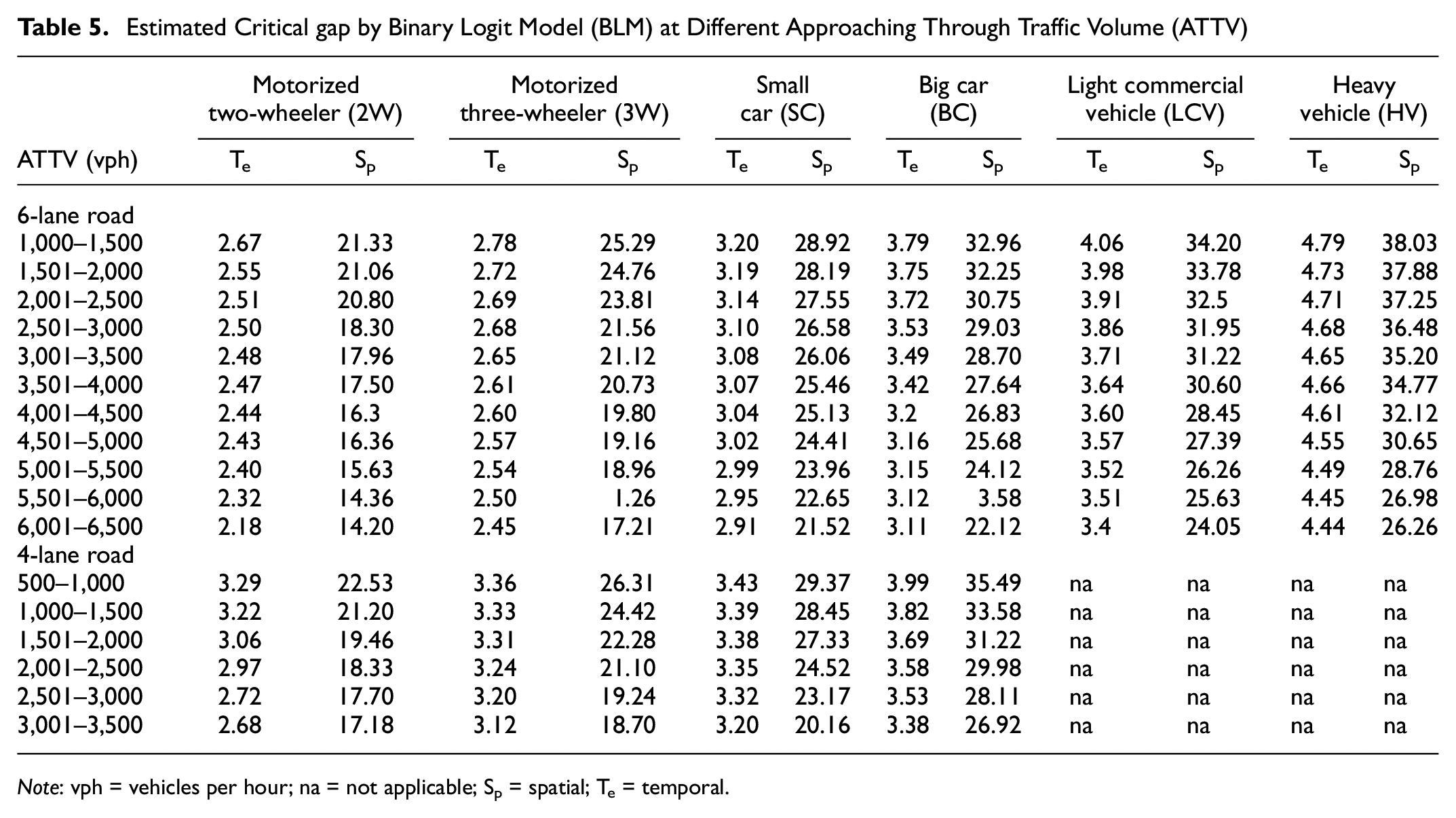
Note: vph = vehicles per hour; na = not applicable; S_p = spatial; T_e = temporal.

After estimating the critical gaps for all the categories of vehicles at different ATTV, an effort was made to compute the BLM’s success rate for prediction of critical gaps. Table 6 shows the success values for predicting U-turning vehicles’ gap acceptance characteristics for all the developed models using BLM. From the table, it can be seen that the overall prediction success rate for the temporal and spatial critical gap at 6-lane roads ranges from 84.30 to 95.90 and 76.30 to 91.90, respectively, and prediction success value for the temporal and spatial critical gap at 4-lane roads ranges from 72.95 to 97.90 and 91.00 to 94.40, respectively.

Table 6.

Prediction Results for Binary Logit Model (BLM) at 1,000 to 1,500 vehicles per hour (vph) Approaching Through Traffic Volume (ATTV)

	Temporal				Spatial
Vehicle type	Field observation	Model prediction		Correct prediction (%)	Field observation	Model prediction		Correct prediction (%)
Vehicle type	Field observation	Rejected	Accepted	Correct prediction (%)	Field observation	Rejected	Accepted	Correct prediction (%)
6-lane road
Motorized two-wheeler (2W)	Rejected	68	10	87.20	Rejected	72	6	92.90
	Accepted	13	66	83.50	Accepted	8	71	89.90
	Total			85.40	Total			91.90
Motorized three-wheeler (3W)	Rejected	38	9	80.60	Rejected	40	7	85.10
	Accepted	4	29	87.90	Accepted	3	30	90.90
	Total			84.30	Total			88.00
Small car (SC)	Rejected	91	6	93.80	Rejected	79	18	81.40
	Accepted	5	105	95.50	Accepted	11	99	90.00
	Total			94.70	Total			86.00
Big car (BC)	Rejected	65	3	95.60	Rejected	65	3	95.60
	Accepted	3	74	96.10	Accepted	9	68	88.30
	Total			95.90	Total			91.70
Light commercial vehicle (LCV)	Rejected	23	2	92.00	Rejected	18	7	72.00
	Accepted	1	33	97.10	Accepted	7	27	79.40
	Total			94.90	Total			76.30
Heavy vehicle (HV)	Rejected	22	3	88.00	Rejected	21	4	84.00
	Accepted	2	32	94.10	Accepted	1	33	97.10
	Total			91.50	Total			91.50
4-lane road
Motorized two-wheeler (2W)	Rejected	151	36	80.70	Rejected	173	14	92.51
	Accepted	64	127	66.50	Accepted	19	172	90.05
	Total			73.50	Total			91.28
Motorized three-wheeler (3W)	Rejected	29	11	72.50	Rejected	36	4	90.00
	Accepted	15	41	73.20	Accepted	4	52	92.90
	Total			72.90	Total			91.45
Small car (SC)	Rejected	49	2	96.10	Rejected	43	8	84.43
	Accepted	2	43	95.60	Accepted	5	40	88.88
	Total			95.80	Total			86.65
Big car (BC)	Rejected	55	1	98.20	Rejected	50	6	89.30
	Accepted	1	38	97.40	Accepted	4	35	89.74
	Total			97.90	Total			89.52

Comparison of Critical Gap Estimated in Different Studies

As mentioned earlier, it is a difficult task to estimate the critical gap directly in the field. Therefore, various models and methods have been developed by different researchers. Most developed methods have been carried out in homogeneous traffic conditions where vehicular traffic follows lane discipline, and the rule of priority is always respected. But in Indian conditions, violation of priority rule and disobeying lane discipline is a common sight on the road. The present study assessed critical gap values of U-turning vehicles at 6-lane and 4-lane roads. Additionally, the critical gap values were also estimated at varying ATTV. But all the previous research has estimate critical gap only for one type of vehicle, namely car, and for a particular traffic volume. Therefore, the authors have compared the critical gap of cars and the detailed comparative findings have been presented in Table 7.

Table 7.

Cross Country Comparison of Estimated Critical Gap

			Difference in critical gap values obtained by different methods and the present study (%)
Name of the study	Country	Critical gap (s)	Modified Raff method (MRM)	Ashworth	Binary logit model (BLM)	Occupancy time (OT)
6-lane
Estimated critical gap			2.79 s	2.70 s	3.06 s	3.9 s
Liu et al. ( 14 )	U.S.	5.60	50.18	51.79	45.36	30.18
Aldian and Taylor ( 25 )	Australia	6.46	56.81	58.20	52.63	39.47
Al-Masaeid ( 16 )	Jordan	6.72	58.48	59.82	54.46	41.82
Jenjiwattanakul and Sano ( 7 )	Thailand	5.00	44.20	46.00	38.80	21.80
4-lane
Estimated critical gap			3.38 s	3.80 s	3.34 s	4.29 s
Liu et al. ( 43 )	U.S.	6.65	49.17	42.86	49.77	35.49

Table 7 provides the difference in the percentage of critical gap found by all the methods utilized in this study and the critical gap values reported in other studies. From the table, it can be concluded that critical gaps found in this study are smaller compared with the other studies in both 6-lane and 4-lane roads. The lower value of the critical gap is observed because of U-turning drivers’ aggressive driving behavior in Indian conditions, which allows them to accept shorter gaps by forcefully entering the MBMO area to complete the U-turn. A similar observation was made by Ashalatha and Chandra ( 5 ). Furthermore, the difference in the percentage of critical gap values in the present study compared with other studies, as tabulated in Table 7, gives an idea of the performance of various critical gap estimation methods. The results tabulated in Table 7 indicate that the OT method provides the critical gap values closest to the critical gap values found in published literature compared with all the other methods considered in the present study.

Conclusions

The present research deals with the analysis of the gap acceptance behavior of vehicles taking U-turns at MBMOs by collecting videographic data from 14 MBMO locations. The main objective of this study is to find the temporal and spatial critical gaps of U-turning vehicles at different ATTV. Critical gap is one important parameter capacity estimation at MBMOs, and it cannot be directly measured in the field. Therefore, numerous techniques have been developed by researchers for critical gap estimation. Four different methods—MRM method, Ashworth method, OT method, and BLM method—have been employed for the estimation of the spatial and temporal critical gaps. The calculated critical gap was found to vary for different types of U-turning vehicles. This could be because of the presence of a wide difference in the physical and mechanical features of U-turning vehicles. Moreover, critical gaps for all vehicles at varying ATTV were estimated. It was observed that the critical gap decreases with an increase in ATTV. A possible reason for this could be that, as the ATTV increases, the U-turning vehicles are forced to wait for longer at MBMOs (compared with lower ATTV) which makes the drivers of U-turning vehicles frustrated so they try to make a U-turn aggressively by accepting a gap which might not be large enough to complete the maneuver. Minor-street drivers tend to perceive spatial gap more precisely compared with the temporal gap in the conflicting stream in which they seek a gap to complete the required maneuver. Therefore, spatial gap plays a very important role in affecting the safety of the minor-street vehicles during merging or crossing maneuvers. Therefore, in this study, the authors have also calculated U-turning vehicles’ spatial critical gap by different methods. The critical gap values estimated by established methods in heterogenous conditions are found to be smaller than the critical gap values reported in other studies under homogeneous traffic conditions. The lower value of the critical gap indicates the aggressive driving behavior of drivers in developing countries in general and Indian conditions in particular. Additionally, the OT method was found to provide the closest critical gap values to the published literature compared with other methods. This study’s outcomes can be employed for capacity estimation for U-turns at MBMOs in both heterogeneous and homogeneous traffic conditions.

The present methodology can assist the practicing engineer in managing the traffic efficiently at MBMOs. The effects of the vehicular composition of ATT, the presence of pedestrians, and gap acceptance behavior of longer wheelbase U-turning vehicles have not been considered in this study. U-turning vehicles with longer wheelbase may need to find a gap between more than two vehicles. Smaller vehicles accept a single gap, whereas longer wheelbase vehicles may have to accept multiple gaps between different vehicles present in different lanes to complete the U-turn. The present paper has not considered these parameters for estimation of the critical gap of different categories of U-turning vehicles; therefore, these limitations have been proposed as the future scope of this study.

Footnotes

Author Contributions

The authors confirm contribution to the paper as follows: study conception and design: T. Khan, S. Mohapatra; data collection: T. Khan, A. Vivek; analysis and interpretation of results: T. Khan, S. Mohapatra; draft manuscript preparation: T. Khan, A. Vivek, S. Mohapatra. All authors reviewed the results and approved the final version of the manuscript.

Declaration of Conflicting Interests

The author(s) declared no potential conflicts of interest with respect to the research, authorship, and/or publication of this article.

Funding

The author(s) disclosed receipt of the following financial support for the research, authorship, and/or publication of this article: T. Khan and A. Vivek of the manuscript are thankful to the fellowship provided by Government of India for carrying out research at IIT(ISM) Dhanbad.

ORCID iD

Smruti Sourava Mohapatra

Data Accessibility Statement

Some videographic data could be provided by the corresponding author on request with a proper justification.

References

Dash

Mohapatra

S. S.

Dey

P. P.

Estimation of Critical Gap of U-turns at Uncontrolled Median Openings. Transportation Letters, Vol. 11, No. 5, 2018, pp. 1–12.

Mohanty

Dey

P. P.

Modelling the Major Stream Delay Due to U-turns. Transportation Letters, Vol. 11, No. 9, pp. 1–8.

Khan

Mohapatra

S. S.

Modelling Lateral Merging Position of Vehicles in Divided Urban Roads. Current Science, Vol. 120, No.11, 2021, pp. 1768’1777.

Sil

Mohapatra

S. S.

Dey

P.P.

Chandra

Merging Process of U-turns at Uncontrolled Median Openings Under Mixed Traffic Conditions. Transport, Vol. 33, No. 2, 2016, pp. 370–379.

Ashalatha

Chandra

Critical Gap Through Clearing Behavior of Drivers at Unsignalised Intersections. KSCE Journal of Civil Engineering, Vol. 15, 2011, pp. 1427–1434.

Mohapatra

S. S.

Dey

P. P.

Chandra

Conflicting Volume for U-turns at Uncontrolled Median Openings. Proceedings of the Institution of Civil Engineers-Transport, Vol. 169, No. 4, 2016, pp. 195’204.

Jenjiwattanakul

Sano

Effect of Waiting Time on the Gap Acceptance Behavior of U-turning Vehicles at Midblock Median Openings. Journal of the Eastern Asia Society for Transportation Studies, Vol. 9, 2011, pp. 1601–1613.

Pawar

D. S.

Patil

G. R.

Minor-street Vehicle Dilemma While Maneuvering at Unsignalized Intersections. Journal of Transportation Engineering, Part A: Systems, Vol. 143, No. 8, 2017, p. 04017039. https://doi.org/10.1061/JTEPBS.000-0066

Khan

Mohapatra

S. S.

Lateral Placement Characteristics of U-turning Vehicles: A Statistical Investigation. Transportation in Developing Economies, Vol. 6, No. 1, 2020, pp. 1–12.

10.

Khan

Mohapatra

S. S.

Effect of Operational Attributes on Lateral Merging Position Characteristics at Mid-Block Median Opening. Transportation Letters, Vol. 13, No. 2, 2021, pp. 83–96.

11.

Patil

G. R.

Pawar

D. S.

Temporal and Spatial Gap Acceptance for Minor Road At Uncontrolled Intersections in India. Transportation Research Record: Journal of the Transportation Research Board, 2014. 2461(1): 129–136.

12.

Kadali

B. R.

Vedagiri

Evaluation of Pedestrian Accepted Vehicle Gaps with Varied Roadway Width under Mixed Traffic Conditions. Transportation Letters, Vol. 11, No. 9, 2017, pp. 1–8.

13.

Ashworth

Green

B. D.

Gap Acceptance at an Uncontrolled Intersection. Traffic Engineering Control, Vol. 7, 1966, pp. 676–678.

14.

Liu

J. J.

Cao

Capacity of U-turns at Unsignalized Median Openings on Six-Lane Streets. Transportation Research Record: Journal of the Transportation Research Board, 2009. 2130(1): 59–65.

15.

Pawar

D. S.

Patil

G. R.

Chandrasekharan

Upadhyaya

Classification of Gaps at Uncontrolled Intersections and Midblock Crossings Using Support Vector Machines. Transportation Research Record: Journal of the Transportation Research Board, 2015. 2515: 26–33.

16.

Al-Masaeid

H. R.

Capacity of U-turn at Median Openings. Institute of Transportation Engineers, ITE Journal, Vol. 69, No. 6, 1999, pp. 28–30.

17.

Mohapatra

S. S.

Dey

P. P.

Estimation of U-turn Capacity at Median Openings. Journal of Transportation Engineering, Part A: Systems, Vol. 144, No. 9, 2018, p. 04018049.

18.

Raff

M. S.

Hart

J. W.

A Volume Warrant for Stop Signs. Eno Foundation for Highway Traffic Control, Saugatuck, CT, 1950.

19.

Velan

S. M.

Van Aerde

Gap Acceptance and Approach Capacity at Unsignalized Intersections. ITE Journal, Vol. 3, 1966, pp. 40–45.

20.

Highway Capacity Manual, 1985. Transportation Research Board. National Research Council, Washington, D.C., 1985.

21.

Highway Capacity Manual, 2000. Transportation Research Board. National Research Council, Washington, D.C., 2000.

22.

Highway Capacity Manual, 2010. Transportation Research Board. National Research Council, Washington, D.C., 2010.

23.

Bunker

J. M.

Novel Methods and the Maximum Likelihood Estimation Technique for Estimating Traffic Critical Gap. Journal of Advanced Transportation, Vol. 48, No. 6, 2012, pp. 542–555.

24.

Brilon

Koenig

Troutbeck

R. J.

Useful Estimation Procedures for Critical Gaps. Transportation Research Part A: Policy and Practice, Vol. 33, No. 3–4, 1999, pp. 161–186.

25.

Aldian

Taylor

M. A. P.

Selecting Priority Junction Traffic Models to Determine U-turn Capacity at Median Opening. Eastern Asia Society for Transportation Studies, Vol. 3, No. 2, 2001, pp. 101–113.

26.

Tian

Z. Z.

Troutbeck

R. R. J.

Kyte

Brilon

Vandehey

Kittelson

Robinson

A Further Investigation on Critical Gap and Follow-up Time. Transportation Research Circular E-C018. Proc., 4th International Symposium on Highway Capacity, Maui, Hawaii, 2000, pp. 397–408.

27.

Ogallo

Jha

Methodology for Critical-Gap Analysis at Intersections with Unprotected Opposing Leftturn Movements. Journal of Transportation Engineering, Vol. 140, No. 9, 2014, p. 04014045.

28.

Equilibrium of Probabilities for Estimating Distribution Function of Critical Gaps at Unsignalized Intersections. Transportation Research Record: Journal of the Transportation Research Board, 2012. 2286: 49–55.

29.

Dutta

Ahmed

M. A.

Gap Acceptance Behavior of Drivers at Uncontrolled T-Intersections Under Mixed Traffic Conditions. Journal of Modern Transportation, Vol. 26, No. 2, 2018, pp. 119–132.

30.

Troutbeck

R. J.

Estimating the Mean Critical Gap. Transportation Research Record: Journal of the Transportation Research Board, 2014. 2461: 76–84.

31.

Paul

Ghosh

Speed-Based Proximal Indicator for Right-Turn Crashes at Unsignalized Intersections in India. Journal of Transportation Engineering, Part A: Systems, Vol. 144, No. 6, 2018, p. 04018024.

32.

Pollatschek

M. A.

Polus

Livneh

A Decision Model for Gap Acceptance and Capacity at Intersections. Transportation Research Part B: Methodological, Vol. 36, No. 7, 2002, pp. 649–663.

33.

Sangole

J. P.

Patil

G. R.

Patare

P. S.

Modelling Gap Acceptance Behavior of Two-Wheelers at Uncontrolled Intersection Using Neuro-Fuzzy. Procedia-Social and Behavioral Sciences, Vol. 20, 2011, pp. 927–941.

34.

Mohan

Chandra

Critical Gap Estimation at Two-Way Stop-Controlled Intersections Based on Occupancy Time Data. Transportmetrica A: Transport Science, Vol. 14, No. 4, 2018, pp. 316–329.

35.

Mohapatra

S. S.

Dey

P. P.

Chandra

Modeling the Critical Position of U-turning Vehicles at Uncontrolled Median Openings. KSCE Journal of Civil Engineering, Vol. 20, No. 1, 2016, pp. 411–420.

36.

Mohapatra

S. S.

Dey

P. P.

Lateral Placement of U-turns at Median Openings on Six-Lane Divided Urban Roads. Transportation Letters, Vol. 7, No. 5, 2015, pp. 252–263.

37.

Pawar

D. S.

Patil

G. R.

Critical Gap Estimation for Pedestrians at Uncontrolled Mid-Block Crossings on High-Speed Arterials. Safety Science, Vol. 86, 2016, pp. 295–303.

38.

Serag

M. S.

Gap-Acceptance Behavior at Uncontrolled Intersections in Developing Countries. Malaysian Journal of Civil Engineering, Vol. 27, 2015, pp. 80–93.

39.

Dissanayake

J. J.

Ping

Y. I.

Driver Age Differences in Day and Night Gap Acceptance Capabilities. IATSS Research, Vol. 26, No. 1, 2002, pp. 71–79.

40.

Ashworth

A Note on the Selection of Gap Acceptance Criteria for Traffic Simulation Studies. Transportation Research, Vol. 2, No. 2, 1968, pp. 171–175.

41.

Ashworth

The Analysis and Interpretation of Gap Acceptance Data. Transportation Science, Vol. 4, 1970, pp. 270–280.

42.

Ben-Akiva

M. E.

S. R.

Lerman

Discrete Choice Analysis: Theory and Application to Travel Demand. MIT Press, Cambridge, MA, 1985.

43.

Liu

Wang

Sokolow

Headway Acceptance Characteristics of U-turning Vehicles at Unsignalized Intersections. Transportation Research Record: Journal of the Transportation Research Board, 2007. 2027: 52–57.