Evaluation of the Operational Effects of Autonomous and Connected Vehicles through Microsimulation

Abstract

Proper evaluation of traffic operations integrating connected and autonomous vehicles (CAVs) requires accurate representation of these emerging technologies in microscopic simulation. This paper evaluates the ability of microscopic simulator PTV-VISSIM (Version 10.0) to simulate CAVs, and presents a comprehensive CAV model extension. In addition, emissions modeling is integrated with VISSIM to calculate real-time energy and emission estimates. The evaluation of VISSIM revealed that its internal CAV modeling has several limitations, such as modeling connectivity and complex vehicle behavior. For external modeling, there are two available VISSIM interfaces. The Component Object Model (COM) Application Programming Interface (API) is the superior approach for fetching data and modeling connectivity, whereas the External Driver Model (EDM) is a better tool for lateral and longitudinal control. The simulation extension developed leveraged both interfaces. An isolated signalized intersection was simulated to demonstrate the impact of connected vehicle (CV), autonomous vehicle (AV), and CAV traffic on speed, delay, and travel time. In addition, trajectory data, combined with the Motor Vehicle Emission Simulator (MOVES) method, were utilized to obtain energy, fuel consumption, and greenhouse gas emissions. The results show that CAVs result in net improvement in travel time and speed. However, emissions did not follow the same trend. While increasing AV penetration rates resulted in emissions reductions, increasing CV and CAV penetration rates resulted in higher emissions. While the CV logic chosen for testing seeks to maximize the likelihood of vehicle arrival-on-green, the algorithm likely results in increased variations in second-by-second accelerations, leading to overall higher emissions.

Keywords

operations traffic simulation automated/autonomous/connected vehicles car-following emission microscopic traffic simulation vehicle trajectory traffic signal systems V2I

Significant improvements in autonomous vehicle technologies as well as their connectivity and interaction with future generation traffic systems are expected to create a perfect storm in how vehicles will navigate through city roads and highways. When considering these emerging vehicle technologies, they may be autonomous (AV), connected (CV), or connected and autonomous (CAV).

AVs can operate on their own and do not require a human driver. They can operate using a variety of sensors such as GPS, lidar, radar, and smart cameras, as well as terrain information. CVs can communicate with surrounding vehicles and infrastructure using wireless communications. For example, the U.S. Department of Transportation (DOT) CV research program aims to enable wireless communications among vehicles, infrastructure, and personal communications devices ( 1 ). The program is currently focusing on pilot deployments to implement existing research concepts and encourage further innovation. Initial CV technology deployments seek to warn drivers of impending dangers while the vehicle is controlled by a human driver; however, applications in operations, sustainability, and access management are also being explored. A vehicle may have both AV and CV capabilities; such vehicles are called CAVs.

It is highly likely that soon CVs, AVs, and CAVs will be operating side by side in large numbers on our nation’s highways, along with conventional (CNV) vehicles. This creates many opportunities for improving surface transportation efficiency and safety. For example, the U.S. DOT Multimodal Intelligent Traffic Signal Systems (MMITSS) initiative aims to provide a comprehensive traffic information framework to service all transportation modes, including general vehicles, transit, emergency vehicles, freight fleets, and pedestrians and bicyclists in a CV environment.

Further, according to the National Transportation Operations Coalition ( 2 ), delays at traffic signals account for 5% to 10% of all traffic delay on major roadways and contributed an estimated 25% to the increase in total highway traffic delays during the past 20 years. Traffic signal timing improvements have the potential to significantly benefit the transportation system. One source of delay at signals is inefficient green time utilization in response to fluctuating demand. Another source is driver-reaction-related delays, including start-up delay. The use of autonomous and CV technology has the potential to reduce the impact of these two factors, through the use of its communication capability as well as the potential to fully control AV trajectories. However, existing simulation tools are not able to accurately replicate the functionality of CAVs (3, 4). Therefore, the impact of various strategies and market penetrations on mobility and the environment cannot be accurately assessed. There are two limitations with existing tools: inability to accurately replicate CAVs ( 3 ) and lack of framework to simulate various types of AV and CV models ( 4 ). Do et al. ( 4 ) present a table of recent studies simulating CAVs. There are two types of studies in the literature:

The studies that deploy their AV/CV models in independently developed coding environments, which are not suitable to “plug and play” other AV/CV models or for large-scale commercialization

The studies that change or calibrate model parameters in existing commercially available simulators to mimic AV behavior. Such models are susceptible to assumptions and limitations of the original model.

The goal of this paper is to develop a robust microscopic simulation extension to allow the evaluation of traffic operational quality considering the presence of CAVs. In this study, we do not develop or calibrate any models. Our focus in this study is to develop and present a framework to simulate (plug and play) AV and CV models of any kind. This is accomplished with the following objectives:

Evaluate the microscopic simulator VISSIM’s ability to simulate CAVs

Develop a comprehensive simulation extension to represent CAVs in VISSIM

Integrate emissions modeling to calculate real-time energy and emission estimates

Assess traffic operational and environmental performance measures for various CAV levels

Among microsimulation packages, the VISSIM package provided by PTV is one of the most broadly used by traffic practitioners and researchers ( 3 ). Some of the reasons for the popularity of this package are its realistic interface, easy use, and flexibility for development. For instance, VISSIM allows users to develop new control strategies or test new driving behaviors by means of an application programming interface (API) called COM. Based on studies in the literature (3, 4) and the strength of its features, we chose VISSIM 10.0 as a candidate in this study. The first half of this paper discusses VISSIM’s capabilities to model CAVs, followed by the development of a comprehensive simulation extension to model CAVs using VISSIM’s Component Object Model (COM) Application Programming Interface (API) and External Driver Model (EDM). The second half presents simulation results related to traffic operational quality, followed by emissions modeling and the respective results.

Evaluation of VISSIM Capabilities to Replicate Autonomy and Connectivity

VISSIM can replicate various types of vehicles (with characteristics that can be modified by the user). To simulate CAVs, one approach is to introduce a vehicle type that represents CAVs and attribute to it the respective behavior and characteristics. For this “internal” modeling, internal parameters of the behavioral models in VISSIM are adjusted to reflect AV behavior. This can be achieved by calibrating VISSIM’s car-following (and other) parameter settings for the designated CAV vehicle type.

Another approach is to model CAVs “externally,” that is, through additional modules (COM API and EDM) utilizing custom algorithm and code development. The next two sections describe each of these two approaches in more detail.

Modeling CAVs Internally

Internal parameters of the behavior models in VISSIM (10.0) can be adjusted to model AV-related features without any external or API programming. This can be achieved by changing VISSIM’s default settings for parameters such as those related to car following, lane changing, and speed. This approach provides a full evaluation to assess changes in the selected parameters, but it is limited to modeling AVs with preset parameters.

The car-following model in VISSIM is based on research by Wiedemann and Reiter ( 5 ). The basic premise of the Wiedemann model states that a vehicle is in one of four states of car following: free, approaching, following, or braking. The following state changes when a threshold based on speed difference and distance difference between the lead and following vehicles is crossed.

The Wiedemann 99 car-following model was developed to provide greater control of the car-following characteristics for freeway modeling in VISSIM ( 6 ). The Wiedemann 99 model consists of 10 calibration parameters (CC0 to CC9). In addition, there are several parameters for modifying for lane change behavior: safety distance reduction factor, maximum deceleration, advanced merging, and cooperative lane change factors. While this paper utilizes VISSIM 10, it is recognized that in VISSIM 2021 a parameter calibration set has been developed under the CoExist Project (www.h2020-coexist.eu/) that reflects several AV behaviors; however, this calibrated AV behavior remains limited to those attributes that may be influenced by existing parameters.

Changes in these internal parameters can be used to reflect simple first-order behaviors of AVs (for example, lower standstill distances and lower lateral distances to reflect AV platooning). However, more complex features such as vehicles’ longitudinal and lateral movement control, vehicle-to-vehicle (V2V) communication, and vehicle-to-infrastructure (V2I) communication cannot be modeled through changes in internal parameters.

Modeling CAVs Externally

Three external VISSIM interfaces can be used to enable modeling CAV behaviors:

COM Application Programming Interface (API);

EDM using DriverModel.dll “dynamic link library” function;

DrivingSimulator.dll that connects with VISSIM simulation in real-time.

COM API

The COM script has access to nearly all data inside VISSIM, and can be made visible in a list window. Certain simulation parameters such as acceleration and headway are only readable, whereas parameters such as desired speed and desired lane are both readable and writable. Thus, COM may be used to enable changes to driving behavior and vehicle movement parameters, but may not be utilized to explicitly control a specific vehicle’s immediate actions during runtime. The COM API does not depend on a certain programming language. COM objects can be developed in a wide range of programming and scripting languages.

External Driver Model (EDM)

The EDM is an external driver model compiled in C++ to substitute the VISSIM default driver model. VISSIM passes the current state of a vehicle and its surroundings to a user-defined dynamic link library file (DriverModel.dll), which then computes the “reaction” of the vehicle based on this information. Thus, EDM may be used to specifically control the movements of a given vehicle, unlike COM. VISSIM allows some or all vehicles to be modeled with the DriverModel.dll. The DriverModel.dll may be used to specify driving behaviors based on CAV logic.

DrivingSimulator.dll Interface

This interface allows testing of the interaction between externally controlled vehicles or pedestrians in VISSIM (also known as “human-in-the-loop” simulation). All decisions and calculations of externally controlled vehicles have to be specified, and are based on the reaction to “other” vehicles in the simulation. Each vehicle moves through the VISSIM network based on simulator instructions, that is, steering movements and acceleration. Other vehicles “react” to what the external vehicle is doing.

Functionality Evaluation of the VISSIM External Interfaces

This evaluation is conducted to assess the capability of the two VISSIM external interfaces (COM API and EDM) to control CAV longitudinal and lateral movements. As discussed in the previous section, the DrivingSimulator.dll Interface requires a separate entity to control the vehicle (for example, a driving simulator) and therefore this approach is not examined further. Only the COM API and EDM are evaluated in this section.

While both the COM API and the EDM enable users to model driving externally, there are certain functional differences.

Data Fetching

COM API has real-time read access to most of the network elements, and write access to many elements. EDM provides data (acceleration, speed, position, etc.) related only to the subject vehicle and neighboring vehicles.

Longitudinal Movement Control

EDM allows users to control longitudinal movement by updating a vehicle’s “desired acceleration” parameter. Through the COM API a user may update a vehicle’s desired speed, which results in a lag in implementation, or update a vehicle location which ignores the acceleration and speed change process, resulting in non-realistic trajectories.

Lateral Movement Control

EDM allows users to completely model lateral movement, whereas the COM API only allows users to set the desired lane where the lane change process is carried out by VISSIM.

Development of CAV Functionality in VISSIM

As seen from the VISSIM COM and EDM functionality in the previous section, the COM API is the superior approach for fetching data and modeling connectivity, whereas EDM is a better tool for lateral and longitudinal control. For many applications the data received by the EDM are not sufficient to model CAV behavior, and additional data retrievable by the COM API are required. Thus, both the EDM and the COM capabilities are needed to model CAVs.

As shown in Figure 1, in each time step the following actions occur:

The COM API data-fetching function reads data from VISSIM required to determine acceleration for a given CV, AV, or CAV in the next time step.

The vehicle logic component written into the COM API calculates the CV, AV, or CAV acceleration for the next time step.

The COM API outputs accelerations of each CV, AV, or CAV to a .txt file.

The EDM reads the .txt file.

The EDM implements acceleration of the subject vehicle in VISSIM.

Figure 1.

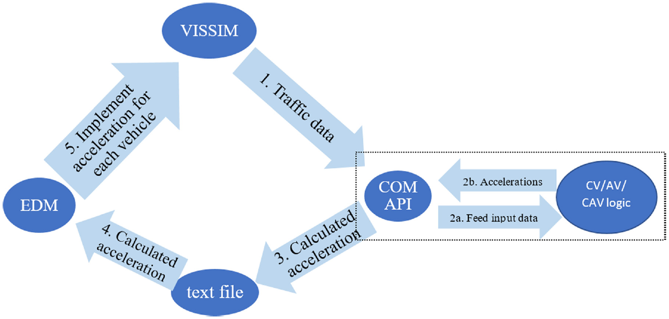
Control framework.

This process is implemented in each time step for all CVs, AVs, or CAVs in the network. Utilizing both the COM API and EDM overcomes the disadvantages of both, creating a more robust platform for CAV modeling.

In this section, an AV model and a CV model are selected from the literature and implemented with the longitudinal control framework developed.

Three simulation networks are built with a mix of:

AV and CNV

CV and CNV

CAV and CNV

AV Model Implementation

In this implementation, a car-following model developed by Talebpour and Mahmassani ( 7 ) is used to replicate the AV logic. The AV logic uses a modified version of the Intelligent Driver Model (IDM) with parameters based on Van Arem et al. ( 8 ) to represent the response of an AV. The model uses three regimes: car following (when a lead vehicle is present), deceleration mode (when the vehicle needs to slow down for a static object such as a red signal), and free driving mode.

When making right or left turns in VISSIM, vehicles must pass through simulation objects called “connectors.” Gap acceptance models are required when using connectors for turning movements. The implemented logic does not include a gap acceptance model; therefore, the driver behavior control is given back temporarily to VISSIM when the AVs need to turn. Figure 2 shows the flowchart of the AV model implementation, and the calculations made in each time step are described below.

Figure 2.

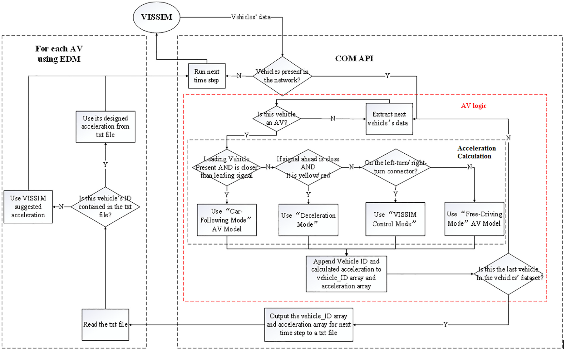
Flowchart of AV logic implementation.

During each time step, the COM API reads traffic data from VISSIM. Traffic data are read for all vehicles in the network. The traffic data are extracted with the command:

“VISSIM.Net.Vehicles.GetMultipleAttributes((‘No’, ‘VehType’, ‘length’, ‘Acceleration’, ‘Speed’, ‘Pos’, ‘Hdwy’, ‘LeadTargNo’, ‘LeadTargType’, ‘DistanceToSigHead’, ‘SignalState’,’Lane’))”

where

“No” is the vehicle’s ID;

“VehType” is the vehicle type (a specific vehicle type is created in VISSIM for AV, CV, and CAVs);

“Pos” is the vehicle’s current position from the start point of its current lane (in meters);

“Hdwy” is the headway distance from its leading vehicle (in meters);

“LeadTargNo” is the ID of the leading target (it could be the ID of signal heads, vehicles, etc.);

“LeadTargType” is the leading target type (if it is a vehicle, signal head, etc.); and

“SignalState” is the state of the leading signal (green, yellow, red).

If the vehicle type is an AV, then based on the car-following regimes as defined in the AV model, the COM API adopts one of four modes (car following, deceleration, free driving, or VISSIM control) to calculate the acceleration of each AV for the next time step. As seen earlier, for each time step and for each vehicle ID, the calculated acceleration is stored in a “.txt” file. The following subsections detail each mode.

Car-Following Mode ( 7 )

The “car-following mode” is executed if the closest leading target with potential influence on behavior is a vehicle (rather than a signal). The acceleration calculation for a vehicle mainly considers two elements: safety constraints and vehicle movement.

Equation 1 calculates the distance the AV should keep from the leading vehicle if the leading vehicle decelerates at its maximum deceleration level:

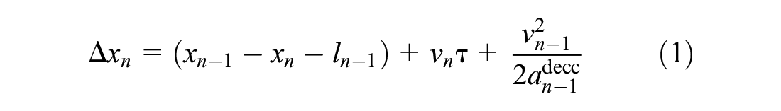
Δ x_{n} = (x_{n - 1} - x_{n} - l_{n - 1}) + v_{n} τ + \frac{v_{n - 1}^{2}}{2 a_{n - 1}^{decc}}

(1)

where

n and n-1 represent the AV and its leader, respectively;

$x_{n}$ is the location of vehicle n;

$l_{n}$ is the length of vehicle n;

$v_{n}$ is the speed of vehicle n;

$τ$ is the reaction time of vehicle n;

$a_{n}^{decc}$ is the maximum deceleration of vehicle n; and

$v_{limit}$ is the speed limit of the road.

In this study, $τ$ = 0.1 s, $a_{n}^{decc} = - 6 m / s^{2}, v_{limit}$ = 20 mph

Equation 2 provides the safe space headway, considering the minimum of safe distance and sensor detection range (a distance of 300 m was used). It assumes that there is a vehicle at a complete stop outside of the sensors’ detection range, which cannot be detected by the sensors at the time of decision-making:

Δ x = min {Sensor Detection range, Δ x_{n}}

(2)

Equation 3 calculates the maximum safe speed ( $v_{\max})$ considering both the safe distance and maximum deceleration:

v_{\max} = \min (\sqrt{- 2 a_{n}^{decc} Δ x}, v_{limit})

(3)

Equation 4 shows the movement model that considers the acceleration of the leading vehicle, the speed difference between the AV and the leading vehicle, and the difference between the real headway and reference headway $S_{ref} :$

a_{n}^{d} (t) = k_{a} a_{n - 1} (t - τ) + k_{v} (v_{n - 1} (t - τ) - v_{n} (t - τ)) + k_{d} (S_{n} (t - τ) - S_{ref})

(4)

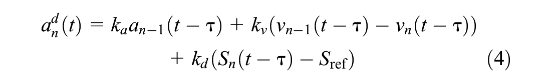
where

$S_{n}$ is the spacing;

$S_{ref}$ is the minimum of minimum distance ( $S_{\min}$ ), following distance based on the reaction time ( $S_{system}$ ), or safe following distance ( $S_{safe}$ );

$a_{n}^{d}$ is the acceleration of vehicle i; and

$k_{a}$ , $k_{v}$ , and $k_{d}$ are model parameters.

Based on the recommendations of Van Arem et al. ( 8 ), $k_{a} = 1.0, k_{v} = 0.58$ , $k_{d} = 0.1$ . In this study, the minimum distance ( $S_{\min})$ is set at 2.0 m.

The following equations calculate $S_{system}$ and $S_{safe} :$

S_{safe} = \frac{v_{n - 1}^{2}}{2} (\frac{1}{a_{n}^{decc}} - \frac{1}{a_{n - 1}^{decc}})

(5)

S_{system} = v_{n} τ

(6)

S_{ref} = \min (S_{safe}, S_{system}, S_{\min})

(7)

a_{n} (t) = min (a_{n}^{d} (t), k (v_{\max} - v_{n} (t), a_{comf})

(8)

where

k is a model parameter; and

$a_{comf}$ is the comfortable acceleration level.

In this study, $k = 1.0$ , and $a_{comf}$ is assumed to be $2.5 m / s^{2}$ .

Deceleration Mode

The deceleration mode is executed when the closest object to a vehicle is a signal head with a red or yellow indication, and the vehicle is approaching it.

Equation 9 calculates the distance to stop $S_{d}$ , that is, the distance required for the vehicle to come to a complete stop if it decelerates at a comfortable deceleration $a_{comf}^{decc}$ :

S_{d} = \frac{1}{2} \frac{V_{n} {(t)}^{2}}{a_{comf}^{decc}}

(9)

where

$S_{d}$ is the acceleration distance;

$a_{comf}^{decc}$ is the comfortable deceleration rate assumed to be $- 3.5 m / s^{2} . a_{n} (t)$ if the distance to signal is less than the distance to stop $S_{d} .$

VISSIM Control Mode

When neither of the two aforementioned situations occur (i.e., the vehicle is influenced neither by a leading vehicle nor by a signal) and the vehicle is making a right or left turn, “gap acceptance models” are required. The authors did not develop a gap acceptance model for this paper; therefore, the AV driver behavior control is temporarily given back to VISSIM to navigate the turn. In this case, the vehicle uses the VISSIM suggested acceleration until it exits the connector.

Free Driving Mode

When the vehicle is not affected by a leading vehicle, a leading signal, or turning, then the “free driving” mode is implemented. In this case the vehicle will aim to maintain or reach the desired speed. Acceleration is estimated as:

a_{n} (t) = k (v_{desired} - v_{n} (t))

(10)

where $k$ is the desired change rate, assumed to be 1 in this study.

This acceleration value is subject to VISSIM’s vehicle dynamics model and its constraints.

Acceleration Implementation through EDM

At each time step, the VISSIM suggested acceleration is stored in the variable “desired_acceleration,” through this command:

“case DRIVER_DATA_DESIRED_ACCELERATION : desired_acceleration = double_value;”

A function is written to check whether a vehicle ID is contained in the first column of the acceleration “.txt” file. If yes, then the vehicle is an AV, so it will use the acceleration from the.txt file. If no, then it is a CNV and it will use the VISSIM suggested acceleration (Figure 2 left part).

CV Model Implementation

The same longitudinal control framework used for AVs is used in the implementation of CV logic. An infrastructure-to-vehicle (I2V) application ( 9 ) allowing the CVs to access signal timing information is used to replicate the CV logic. The CV logic (as developed and recommended by VISSIM) seeks to maximize the likelihood of arrival-on-green by changing a vehicle’s speeds within certain bounds.

It must be noted here that the “CVs” in the VISSIM application example always follow the advice while a true CV would make a choice depending on the driver. This could be modeled by using a factor for driver compliance. However, in this implementation VISSIM logic is used “as is.”

Figure 3 shows a flowchart of the CV model implementation, and the calculations made in each time step are described in this section. The following user-defined attributes are created in the VISSIM COM API to enable CV modeling:

“GreenEnd” is an input attribute which defines the cycle second at which a particular signal group switches from green to amber.

“GreenStart” is an input attribute which defines the cycle second at which a particular signal group switches to green.

“TimeUntilNextGreen” calculates the time until the next green phase starts (this is applicable only for pre-timed control), considering the cycle time and the GreenStart and GreenEnd.

“TimeUntilNextRed” calculates the time until the next red phase starts, considering the GreenStart and GreenEnd.

“SpeedMaxForGreenStart” calculates the maximum speed to arrive at the next green start. If the vehicle drives faster, it will arrive at the signal before the next green time.

“SpeedMinForGreenEnd” calculates the minimum speed to arrive before the next green end. If the vehicle drives slower, it will not make it in the current/next green time.

The CV model implementation considers the following rules:

If the signal ahead is in green, the COM API first calculates if it is possible to arrive at the intersection within the current green phase, by comparing SpeedMinForGreenEnd with desired speed $v_{desired}$ .

If $v_{desired}$ > SpeedMinForGreenEnd, then $v_{desired}$ will remain the same and the vehicle could pass through the intersection during the current green phase at the current desired speed.

If $v_{desired}$ < SpeedMinForGreenEnd, or the signal ahead is red, then COM API will compare $v_{desired}$ with SpeedMaxForGreenStart, to check if the vehicle needs to decelerate to arrive after the next green phase start.

$v_{desired}$ = min ( $v_{desired}$ , SpeedMaxForGreenStart).

After $v_{desired}$ for each vehicle is determined, Equation 10 is used to calculate its acceleration.

The acceleration implementation through EDM for CVs is the same as for AVs, with one difference (Figure 3, left part). When the EDM finds the vehicle ID in the acceleration “.txt” file, it compares the estimated acceleration to the VISSIM suggested acceleration, and uses the lower one (i.e., the vehicle is restricted by both the VISSIM car-following model and the CV logic).

Figure 3.

Flowchart of CV logic implementation.

CAV Model Implementation

The CAV logic combines the AV logic and the CV logic, by replacing the VISSIM car-following model with the AV car-following model in the CV logic. The CAV acceleration is then constrained by both the AV car-following model and the CV model. ( $a_{n} (t) = min (a_{n} {(t)}_{av}, a_{n} {(t)}_{cv}))$ .

Simulations

The AV and CV models described in the previous section were implemented through the COM API and several simulations were run with different combinations of leader and follower vehicles in VISSIM Version 10.0. These vehicles were inserted at different times during the signal cycle to demonstrate and check the implementation of the logic.

Figure 4 shows the results of one such test with the trajectories of a pair of vehicles approaching the stop bar of a signalized intersection. The upstream end of the road segment is 500 ft from the stop bar. When the lead vehicle enters the detection range there are 10 s of green remaining.

Figure 4.

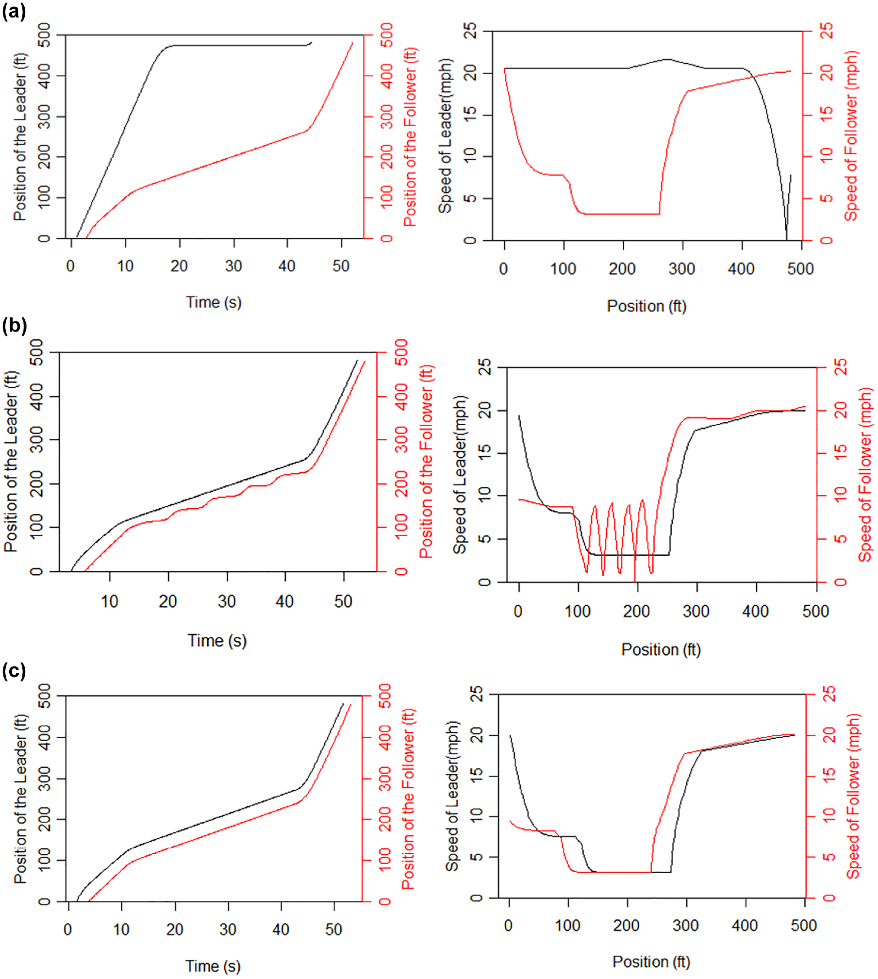
Trajectories of leader and follower vehicles: (a) leader-CNV, follower-CV, (b) leader-CV, follower-CNV, and (c) leader-CV, follower-CV.

In Figure 4a the lead vehicle is a CNV and the follower a CV. The CNV maintains its speed at the speed limit (20 mph) until it approaches the stop bar, and then it decelerates to a complete stop. The CV (the follower) receives the information that the green phase ends soon and it does not have time to cross the stop bar. Therefore it slows down and reaches a lower speed, cruising until the next green, and accelerating later to cross the intersection.

In Figure 4b the lead vehicle is a CV and the follower a CNV. The leading CV decelerates, cruises, and then accelerates to cross the intersection during the next green. The CNV does not have this information and aims to achieve its desired speed, exhibiting oscillation when following the CV which maintains a lower cruising speed.

In Figure 4c both vehicles are CVs. Therefore, they both exhibit the same behavior, and they decelerate to a lower cruising speed before accelerating to cross the intersection during the next green. In this scenario, the following CV does not exhibit any oscillations since both leader and follower are CVs that follow the same trajectory pattern.

The research team conducted several similar tests with vehicle arrivals throughout the cycle, to ensure the individual vehicles behaved as expected. Next, we simulated a four-leg isolated signalized intersection. The research team replicated the signalized intersection of Gale Lemerand Drive and Stadium Road in Gainesville, Florida. The following sections describe the network layout, simulation scenarios, and results.

Simulation Network

Figure 5a provides the study intersection layout. The speed limit is 20 mph for all approaches. Each approach has two lanes with an exclusive left turn bay and a shared lane for through and right turning traffic. Figure 5b provides the network modeled in VISSIM. The width of lanes and the length of the left turn bays were measured using Google maps.

Figure 5.

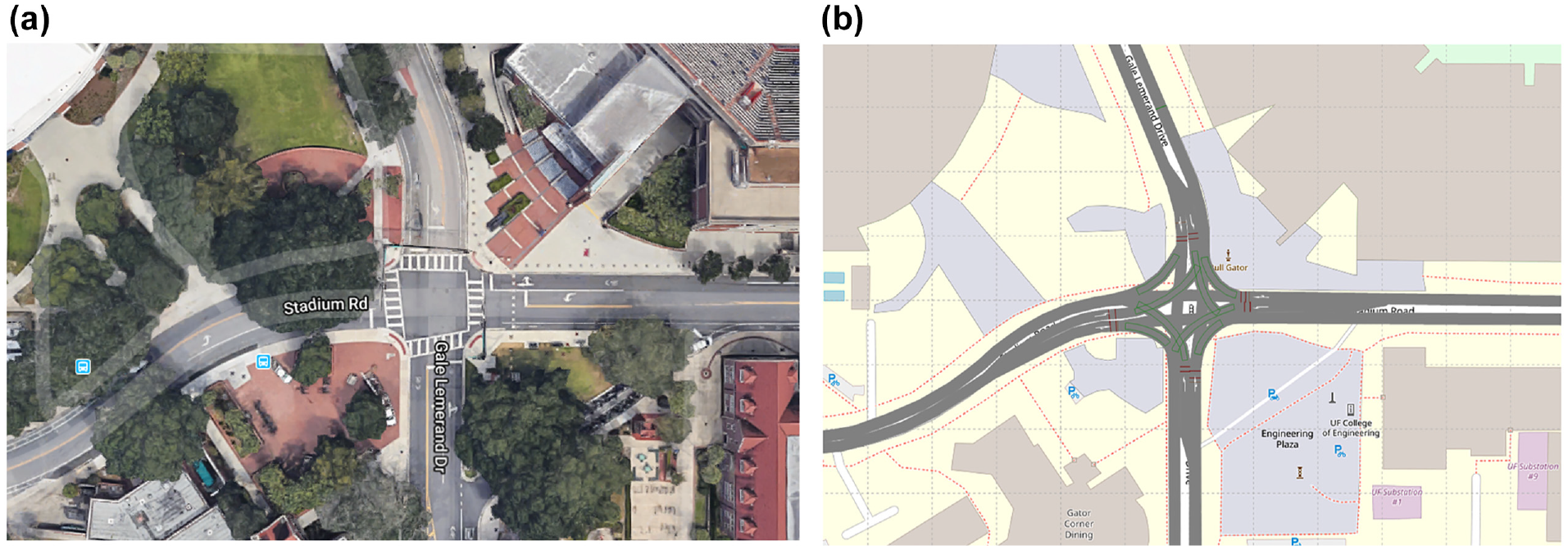
Network layout: (a) network layout satellite view and (b) network layout in VISSIM.

Simulation Scenarios

To understand the impact of CAVs on traffic operations, different penetration rates of AV, CV, or CAV under different volume/capacity (v/c) ratios were replicated. Eighteen scenarios were designed with different combinations of v/c ratio and penetration rate for AV, CV, and CAV each:

V/c ratios used—0.7, 0.85 and 0.9

Penetration rates—0, 0.2, 0.4, 0.6, 0.8 and 1

Each scenario was simulated with five random seeds for 3,600 s with warm-up/-down time of 600 s each.

Simulation Signal Phasing and Timing

For simplicity, the total volume of vehicles and the ratio of turning movements from each approach was kept the same. The ratio was set at 60:30:10 for through, right turns, and left turns, respectively. The total volumes from each approach were 473, 573, and 608, corresponding to v/c ratios of 0.7, 0.85, and 0.9, respectively.

Based on the field data collection, the simulated intersection uses two-phase operation with permitted left turns. Optimal cycle length times were calculated using the HCM6 and rounded to the nearest second, with a minimum allowable cycle of 60 s.

Simulation Results

As described in the previous section, 18 scenarios were developed to replicate various market penetrations for each vehicle type (AV, CV, and CAV). Each of these 54 scenarios (18*3) was simulated five times with different random seeds. The same five random seeds were used across all scenarios to ensure the same traffic arrival pattern for different vehicle types (AV, CV, CAV).

Average travel speed (mph) and average delay (s/veh) for the entire network were obtained for each scenario, and are shown in Figure 6. The following are concluded from the simulation runs:

Increasing penetration rates of CAVs resulted in delay reductions. Scenarios with CAVs showed the highest delay reduction compared with AVs and CVs alone.

Scenarios with AVs result in slightly improved performance at lower traffic volumes (when v/c is 0.7 and 0.85) than the respective scenarios with CVs, as indicated by higher average speed and lower average delay. However, the scenarios with CVs show better network-wide performance than those with AVs at higher demands (i.e., for v/c = 0.9).

The improvements in delay could be attributed to three factors; the reduction in start-up lost time, acceleration of CVs according to the information received, and reduction in driver reaction time.

The results show that a combination of the two technologies (i.e., autonomy and connectivity) yields better performance than either CV or AV on their own.

Figure 6.

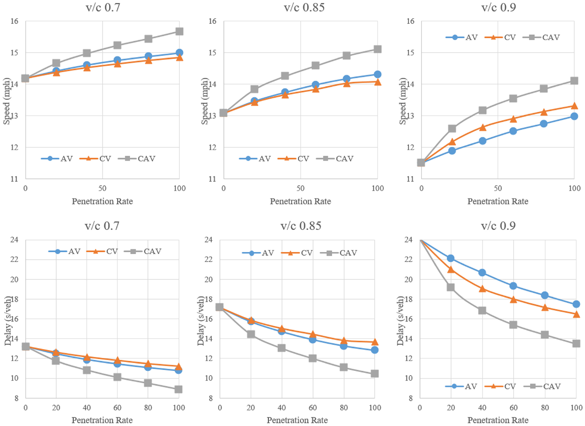
Average speed and delay from VISSIM simulation.

While the simulations show improvements in traffic operational performance, it is also important to consider the environmental impact. In the next section we use the simulation outputs’ evaluated emissions performance for each scenario.

Emissions Modeling

In addition to speed and delay, the differences in emissions under the AV, CV, and CAV scenarios were explored. For brevity, this paper reports carbon dioxide (CO₂) emissions for the eastbound (EB) through vehicles and for the v/c ratios of 0.7 and 0.9.

Data Processing Methodology

Trajectory data, that is, vehicular position over time, are collected for all vehicles during each simulation run and utilized as the underlying data for the CO₂ calculations. For the analysis, the EB roadway is divided into two segments: segment one is upstream of the signal stop bar and is of sufficient length (535 ft) to ensure the entire queue is captured in every simulation scenario, and segment two is downstream of the end of segment one and is of a sufficient length (530 ft) to capture the acceleration of vehicles to their desired speed. Total vehicular CO₂ emissions are estimated using EPA’s Motor Vehicle Emission Simulator (MOVES) model for the 2017 fleet mix. The EPA’s MOVES Model ( 10 ) is used to estimate vehicle energy consumption and emissions given the vehicle’s speed and acceleration. For each second of trajectory data, the speed, acceleration, type of vehicle, and road grade variables are used to calculate vehicle specific power (VSP). The speed, acceleration, and VSP data are then used to identify the relevant MOVES VSP operating mode bin for that second of data. Finally, fuel consumption and emissions are determined for each operating mode bin through the use of MOVES lookup tables. The methodology is provided in detail in Guensler et al. ( 11 ).

The MOVES model is applied at a 1 Hz rate, while the raw trajectory data are available at 10 Hz. Therefore, for this project the median speed for every 10 records of each vehicle is used to condense the 10 Hz data to 1 Hz (i.e., second-by-second). Other methods could be selected for aggregating to a 1 Hz rate, such as mean speed or every tenth data point; however, initial comparisons of such methods showed minimal difference. Median speed was selected as it provides some smoothing of the 10 Hz data while still allowing for fast runtimes, which is critical for real-time applications as discussed elsewhere ( 12 ). The 1 Hz vehicle acceleration is derived from the difference in consecutive median speeds in the condensed trajectory data. Finally, the total emissions for a vehicle are calculated by summing the emissions for every second of the vehicle trip. The calculation of emissions was implemented using Python 3.7 ( 13 , 14 ).

Comparative Analysis and Discussion

Vehicles that enter the model in the first 600 simulation seconds were not included in the analysis, to allow for a simulation warm-up period. Therefore, for all aspects of analysis in this section, only vehicle trips starting at t = 600 s or later and ending at or before t = 3,600 s are considered. For all the boxplots presented in the subsections that follow (Figures 7 and 8), the red square dots represent the mean of the given quantity, the top and bottom of the solid rectangular box represent the 75th percentile and 25th percentile, respectively, and the black line splitting the solid portion of the box into two is the median. Plots presented in the following sections provide data for end-to-end EB trips, that is, segment 1 and segment 2 combined. For brevity, segment specific results, or results from other key performance indicators (KPIs), are not reported in this paper although they may be found in Manjunatha et al. ( 15 ). It was observed that the trends seen in these other results align well with the overall trip results discussed in the following subsections.

Figure 7.

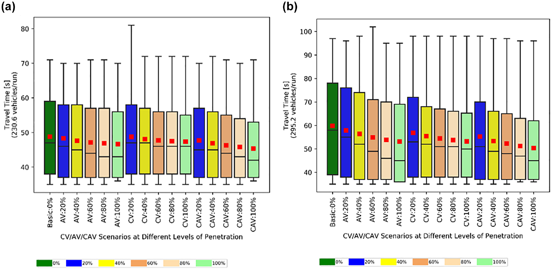
Comparative study: eastbound through vehicle’s travel times for: (a) v/c = 0.7 and (b) v/c = 0.9.

Figure 8.

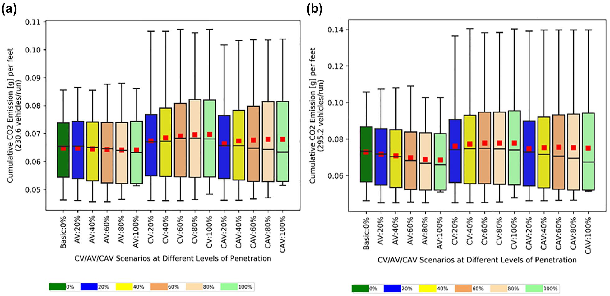
Comparative study: EB-through vehicle’s CO₂ emissions for: (a) v/c = 0.7 and (b) v/c = 0.9.

Travel Time Comparative Analysis

Before presenting CO₂ emissions, travel time results are briefly discussed as these provide for interesting comparison with the emissions. The travel time results are aggregated over five replicate runs. Figure 7, a and b, reflect the EB travel time for v/c’s of 0.7 and 0.9. Both plots show a trend of decreasing mean, median, and 75th percentile travel time with increasing AV, CV, and CAV penetration rates. These trends are more prominent in the AV and CAV results than the CV results. In addition, the travel time interquartile range (IQR), depicted by the vertical length of the boxes in the plots, generally decreases with increasing penetration rates. These trends are somewhat more pronounced under the higher demand level (i.e., v/c = 0.9). Therefore, for all AV/CV/CAV penetration levels, improved travel times and reduced variability are seen at higher penetration rates and volume levels. These results agree well with the previously presented speed and delay findings (Figure 6).

CO₂ Emission (MOVES Estimate) Comparative Analysis

CO₂ results are next presented in a similar format to that of the travel time. To allow for a comparison between routes and scenarios, CO₂ emissions are expressed as emissions per unit distance (in grams per foot) for each individual vehicle.

As seen in Figure 8, the mean and median emissions show a slight reduction with increasing AV penetration. However, mean and median emissions show an increase with increasing CV penetration, while for the CAV cases an increasing penetration rate results in increasing average but decreasing median CO₂ emissions. The emissions IQR also increases with CV and CAV penetration. AV demonstrated lower emissions than CV and CAV at all penetration rates. These trends are consistent at both demand levels.

Based on the speed, delay, and travel time results, it would appear that vehicles should have more efficient route traversal with increasing AV, CV, and CAV penetration. At first glance this would intuitively imply lower emissions with increasing penetration rate, assuming the improved KPIs are a result of fewer stops and acceleration/deceleration events. However, the anticipated emissions improvements were not seen. The next section will further explore these findings.

Emission Analysis: VSP Operating Mode Bin Histogram

Figure 9, a–d, shows the VSP-bin density histograms for CV penetration rates of 0%, 20%, 60%, and 100%, respectively, for v/c = 0.9, simulation random seed = 1, on the EB route. Since the vehicle speed for the network never exceeded 25 mph, no data points were observed beyond VSP-bin 16 (Table A.1 in Xu et al. [ 16 ]). By comparing the plots, it becomes evident that with increasing CV penetration, more data points appear in bin 12 (cruising/acceleration) and fewer data points fall in bins 0 (deceleration), 1 (idle), and 11 (coasting). The CV algorithm has achieved its stated goal; that is, maximizing arrival-on-green, which is seen in the reduction in idle time. However, there is an increase in data points in bin 12, which has a higher emission value than bins 0, 1, and 11, resulting in more overall emissions. It is hypothesized that in the implemented CV logic, the vehicles (CV and non-CV following, as seen in Figure 4) are undergoing more cycles of acceleration and deceleration by undertaking frequent adjustments to their speed to maximize the likelihood of arrival-on-green. This increasing number of changes in acceleration results in higher emissions. However, in the real world there are certain limitations on how fast an acceleration change can be propagated through the drivetrain as well as limitations on the frequency and magnitude of acceleration reversals that are acceptable for driver comfort. It is therefore expected that a successful CV algorithm would smooth out the acceleration profile.

Figure 9.

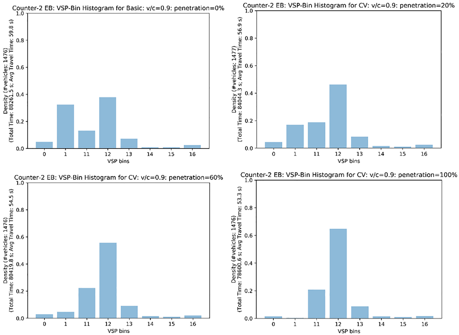
Variations in VSP-bin distribution for eastbound (EB) through vehicles with increasing penetration in CV for v/c = 0.9, simulation random seed = 1: (a) 0% penetration (top left), (b) 20% penetration (top right), (c) 60% penetration (bottom left), and (d) 100% penetration (bottom right).

Possible Causes of Increased Emissions with Higher Penetration Levels of CV

A deeper analysis into the root cause of these trends showed that while the CV logic chosen for testing in the VISSIM simulation environment seeks to maximize the likelihood of vehicle arrival-on-green, the algorithm likely results in increased variations in second-by-second accelerations, leading to overall higher emissions. Examining the trajectories for scenarios with higher penetration levels of CV, we found three possible reasons for higher emissions.

Conventional Vehicle (CNV) Following Behavior

When the lead vehicle is a CV and the follower a CNV, the CNV does not have the same information as the CV. Therefore, instead of slowing down to a lower cruising speed, as the CV does (see Figure 4b), the CNV aims to achieve its desired speed and enters a sharp oscillation pattern around the lower cruising speed of the leader-CV. These oscillations probably contribute to increased emissions, although it is likely this is an artifact of the low speed following behavior rather than expected real-world behavior. That is, it is unlikely that a human-driven vehicle would initiate this rate of acceleration and deceleration to assiduously maintain its desired speed, with most drivers tending to a smoother speed profile. However, this supposition should be further explored with field data.

VISSIM’s CV Movement Logic

When either the leader or the follower is a CV which enters the communication range when the signal is red, VISSIM’s CV logic utilizes a parameter called “SpeedMaxForGreenStart,” which is the maximum speed to arrive at the next green start (details of these calculations are provided in the model implementation section). The calculation of this parameter depends on the green time remaining. While our simulation runs at 0.1 s frequency, the COM API updates this parameter (internally) every 1 s by default (regardless of simulation frequency set). This leads to an approximation of “green time remaining” to the nearest second. This results in “spikes” every half a second (because of rounding) and results in the oscillation pattern shown in Figure 10a. This occurs only when the CV arrives during the red signal. The oscillation can be alleviated by calculating the “SpeedMaxForGreenStart” parameter manually according to the chosen simulation frequency as shown in Figure 10b. Using the VISSIM CV code an acceleration and deceleration profile is again seen that is unlikely in a human-driven vehicle or an AV that has human passengers where such an oscillation could result in significant discomfort. However, for the purposes of demonstration we chose to use VISSIM’s CV code as is, and this may be one of the contributing factors to increased emissions with CVs.

Figure 10.

Optimal speed provided by VISSIM and manually estimated: (a) acceleration of leader-CV and follower-CV with 30 s red remaining (VISSIM’s CV logic) and (b) comparison of VISSIM CV logic and manually estimated speed.

Artifact of Binning

Finally, it is possible that a portion of the results may be an artifact of the binning process used in the MOVES approach. The emissions may be being overestimated; if the vehicle operations are occurring at the boundaries of bins 1, 11, and 12, for example, a minor change in vehicle operations is shifting the emissions calculation from bin 1 to bin 12. Future efforts will explore this potential impact.

Conclusions

This paper evaluated the capability of VISSIM to model CAVs and concluded that internal modeling provides limited access to vehicle/driver behavior parameters and cannot model connectivity. Externally, COM API and EDM have powerful features to enable CAV modeling.

While the COM API has access to all VISSIM data and is helpful in modeling connectivity, it cannot provide direct and accurate longitudinal and lateral movement control. The EDM enables full control of both longitudinal and lateral movements but with limited accessibility to VISSIM data. Therefore, this project developed the ability to simulate CAVs in VISSIM by using COM API to access network elements and EDM to maintain the longitudinal control of vehicles.

The functionality and results of this new procedure are demonstrated by simulating CAVs at a four-legged isolated signalized intersection using VISSIM. A model developed by Talebpour and Mahmassani ( 7 ) was used to replicate the AV logic. The AV logic uses a modified version of the IDM with parameters set based on Van Arem et al. ( 8 ) to represent the response of an AV. VISSIM’s I2V application ( 9 ) allowing the CVs to access signal timing information was used to replicate the CV logic. This CV logic seeks to maximize the likelihood of arrival-on-green by changing a vehicle’s speed within certain parameters.

Several traffic scenarios were simulated (demand levels of v/c = 0.7, v/c = 0.85 and v/c = 0.9, and CV, AV and CAV market penetration rates of 0% to 100%, at 20% increments; each scenario was tested using the same five random seeds). The results show net improvement in traffic operational measures (travel time and speed). Also, CAV, the combination of the two technologies (i.e., autonomy and connectivity) yields better performance than each of the technologies (CV and AV) on its own.

However, emissions did not follow the same trend. While increasing AV penetration rates resulted in emissions reductions, increasing CV and CAV penetration rates resulted in higher emissions. A deeper analysis into the root cause for these trends showed that while VISSIM’s CV logic seeks to maximize the likelihood of vehicle arrival-on-green, the algorithm likely results in oscillation of the second-by-second speeds, leading to overall higher emissions.

Recommendations and Limitations

The paper presents a framework for evaluating AV, CV, and CAV technology in VISSIM, and the ability of such a framework to determine the impact of these technologies on operational and environmental performance. This framework can be used for any model that simulates vehicle movement based on these technologies. While important insights were drawn from this study, they are based on a small highway network, limiting the ability to generalize the findings. Testing of this framework on a larger arterial network and on freeways would provide additional information, particularly related to network-wide effects from AV, CV, and CAV. A more complex network with improved technology algorithms would allow for a more robust analysis. In addition, this project focused on specific AV, CV, and CAV algorithms that replicate vehicle movement. Additional analysis should be conducted to evaluate new algorithms as these become available. Any models that are implemented using the framework presented in this paper should use field data for their 0% penetration scenario to bring realism to their model. The CV model used as an example to demonstrate our framework in this paper only utilizes V2I communication. CAVs are modeled as the sum of AVs and CVs with the limit on acceleration in this paper. V2V connectivity has the potential to enable higher performance. Models utilizing V2V could be tested in the future.

In future work, we plan to incorporate into the simulation extension an intersection optimization algorithm for CAVs, developed by the University of Florida. Further, the emissions could be incorporated along with the existing delay-based objectives into the problem formulation of the optimization.

Footnotes

Author Contributions

The authors confirm contribution to the paper as follows: study conception and design: L. Elefteriadou, M.P. Hunter; data collection: P. Manjunatha, S. Roy; analysis and interpretation of results: P. Manjunatha, M.P. Hunter, A. Guin; draft manuscript preparation: P. Manjunatha, L. Elefteriadou, M.P. Hunter, S. Roy, A. Guin. All authors reviewed the results and approved the final version of the manuscript.

Declaration of Conflicting Interests

The author(s) declared no potential conflicts of interest with respect to the research, authorship, and/or publication of this article.

Funding

The author(s) disclosed receipt of the following financial support for the research, authorship, and/or publication of this article: This project was funded by the U.S. DOT/Region 4 STRIDE University Transportation Center. Project ID is ``STRIDE Project D.

ORCID iDs

Pruthvi Manjunatha

Somdut Roy

Lily Elefteriadou

Angshuman Guin

Michael Hunter

References

Connected Vehicle Pilot Deployment Program. Office of the Assistant Secretary for Research and Technology. https://www.its.dot.gov/pilots/. Accessed December 1, 2021.

Denney

R. W.

Jr. Curtis

Olson

The National Traffic Signal Report Card. ITE Journal, Vol. 82, No. 6, 2012, pp. 22–26.

Gora

Katrakazas

Drabicki

Islam

Ostaszewski

Microscopic Traffic Simulation Models for Connected and Automated Vehicles (CAVs)—State-of-the-Art. Procedia Computer Science, Vol. 170, 2020, pp. 474–481.

Rouhani

O. M.

Miranda-Moreno

Simulation-Based Connected and Automated Vehicle Models on Highway Sections: A Literature Review. Journal of Advanced Transportation, Vol. 2019, 2019, pp. 1–14.

Wiedemann

Reiter

Microscopic Traffic Simulation: The Simulation System Mission. PTV America, Inc., Beaverton, OR, 1991.

Fellendorf

Vortisch

(eds.). Validation of the Microscopic Traffic Flow Model VISSIM in Different Real-World Situations. Presented at 80th Annual Meeting of the Transportation Research Board, Washington, D.C., 2001.

Talebpour

Mahmassani

Influence of Connected and Autonomous Vehicles on Traffic Flow Stability and Throughput. Transportation Research Part C: Emerging Technologies, Vol. 71, 2016, pp. 143–163.

Van Arem

Van Driel

C. J. G.

Visser

The Impact of Cooperative Adaptive Cruise Control on Traffic-Flow Characteristics. IEEE Transactions on Intelligent Transportation Systems, Vol. 7, No. 4, 2006, pp. 429–436.

Evanson

(ed.). Connected Autonomous Vehicle (CAV) Simulation Using PTV Vissim. Proc., 2017 Winter Simulation Conference (WSC), Las Vegas, NV, IEEE, New York, NY, December 3–6, 2017, pp. 4420–4420.

10.

Agency USEP. MOVES and Other Mobile Source Emissions Models. https://www.epa.gov/moves. Accessed December 1, 2021.

11.

Guensler

Liu

Akanser

Kim

Hunter

M. P.

Rodgers

M. O.

Energy Consumption and Emissions Modeling of Individual Vehicles. Transportation Research Record: Journal of the Transportation Research Board, 2017. 2627: 93–102.

12.

Saroj

Roy

Guin

Hunter

Fujimoto

(eds.). Smart City Real-Time Data-Driven Transportation Simulation. Proc., 2018 Winter Simulation Conference (WSC), Gothenburg, Sweden, IEEE, New York, NY, December 9–12, 2018, pp. 857–868.

13.

Python. Python 3.7.0 Release 2018. https://www.python.org/downloads/release/python-370/. Accessed December 1, 2021.

14.

Numpy. Numpy Reference2020. https://numpy.org/doc/stable/reference/index.html. Accessed December 1, 2021.

15.

Manjunatha

Elefteriadou

Hunter

Duan

Letter

Roy

White

C. C.

Postma

Guin

Evaluation of Advanced Vehicle and Communication Technologies through Traffic Microsimulation. STRIDE Project D Final Report. Southeastern Transportation Research, Innovation, Development and Education Center (STRIDE), Gainesville, FL, 2021.

16.

Gbologah

F. E.

Lee

D.-Y.

Liu

Rodgers

M. O.

Guensler

R. L.

Assessment of Alternative Fuel and Powertrain Transit Bus Options Using Real-World Operations Data: Life-Cycle Fuel and Emissions Modeling. Applied Energy, Vol. 154, 2015, pp. 143–159.

Evaluation of the Operational Effects of Autonomous and Connected Vehicles through Microsimulation

Abstract

Keywords

Evaluation of VISSIM Capabilities to Replicate Autonomy and Connectivity

Modeling CAVs Internally

Modeling CAVs Externally

COM API

External Driver Model (EDM)

DrivingSimulator.dll Interface

Functionality Evaluation of the VISSIM External Interfaces

Data Fetching

Longitudinal Movement Control

Lateral Movement Control

Development of CAV Functionality in VISSIM

AV Model Implementation

Car-Following Mode ( 7 )

Deceleration Mode

VISSIM Control Mode

Free Driving Mode

Acceleration Implementation through EDM

CV Model Implementation

CAV Model Implementation

Simulations

Simulation Network

Simulation Scenarios

Simulation Signal Phasing and Timing

Simulation Results

Emissions Modeling

Data Processing Methodology

Comparative Analysis and Discussion

Travel Time Comparative Analysis

CO2 Emission (MOVES Estimate) Comparative Analysis

Emission Analysis: VSP Operating Mode Bin Histogram

Possible Causes of Increased Emissions with Higher Penetration Levels of CV

Conventional Vehicle (CNV) Following Behavior

VISSIM’s CV Movement Logic

Artifact of Binning

Conclusions

Recommendations and Limitations

Footnotes

Author Contributions

Declaration of Conflicting Interests

Funding

ORCID iDs

References

CO₂ Emission (MOVES Estimate) Comparative Analysis