Vehicle Trajectory-Based Calibration Procedure for Microsimulation

Abstract

In practice, traffic engineers and researchers calibrate microscopic driver behavior in microsimulation models using macroscopic inputs (e.g., aggregated traffic throughput) instead of microscopic inputs (e.g., inter-vehicle spacing and acceleration). This mismatch has naturally led to concerns that these models have not accurately captured the microscopic driver behaviors, despite the apparent goodness-of-fit in the macroscopic performance measures. There is renewed interest in trajectory-based calibration for microsimulation models given the recent improvements in data collection and data processing technologies. Toward this end, this project collected aerial vehicle trajectories using cameras attached to drones at three real-world sites (producing 800 ft trajectories) and a helicopter at one site (producing 1.2 mi trajectories). This study used these datasets to develop a new microsimulation model trajectory-based calibration method and calibrated four urban freeway models: I-270, I-15, I-75, and I-95. Next, this study calibrated models of the same four sites using macroscopic data (e.g., average segment speed and throughout). Finally, this study compared the two methods’ calibration accuracy to understand the benefits of the trajectory-based calibration method. The experimental results provided evidence that analysts should not trust traditional calibration methods to produce models with realistic vehicle trajectories. However, explicit integration of trajectories into the calibration process (i.e., hybrid calibration methods) can significantly improve the modeled trajectories’ realism. Calibrated model results were most impressive at I-75, which is the only site that collected data via helicopter, yielding significantly longer trajectories.

Keywords

operations traffic simulation calibration/validation car-following microscopic traffic simulation vehicle trajectory

Simulation is an indispensable tool for transportation professionals. It provides a cost-effective method for predicting the impact of various changes to the transportation system (e.g., land use changes, geometric design alternatives, active traffic management strategies, nonrecurring events, and growing traffic demands over time) on traffic flow and performance (e.g., travel time, speed, and capacity). Microscopic simulation, or microsimulation, provides detailed representation of car-following and lane-changing behaviors for analyses that focus on urban freeway interchanges and corridors. When conducted properly, the combination of lane-specific results, static graphics, moving vehicle animation, and statistical outputs supplies valuable information to decision makers. To ensure analyses are conducted properly, analysts must perform proper model calibration, which is the process of estimating model parameters to represent local conditions more realistically.

Conventional calibration practices (i.e., calibrating to traditional aggregate performance measures, such as speed and volume) may not produce the robust outcomes and accurate models that engineers expect. In one example, a study of six microsimulation models that were well calibrated to aggregate measures produced wildly divergent predictions for future conditions ( 1 ). There are several possible explanations for this observation. Firstly, although these models were developed with best practices in mind, the changes made to the driver behavior parameters to best match current conditions’ aggregate measures may have resulted in unintended impacts to models with different underlying assumptions (e.g., future demand), making those estimates of future conditions unreliable. Conversely, this may also suggest that the calibrated driver behavior models were overfit to current traffic conditions and were not generalizable for other conditions, such as future demand of the same modeled area. Regardless of the explanation, the results of Bloomberg et al. ( 1 ) imply that practitioners may have been focusing on traditional measures at the expense of underlying driver behaviors and vehicle dynamics, possibly leading to less reliable modeling of predictions.

Moreover, the authors are unaware of research conducted to evaluate the accuracy of individual trajectories based on models calibrated using segment-level aggregate performance measures. Thus, it may be possible to demonstrate that simulated vehicle trajectories from microsimulation models calibrated by traditional methods are quite unrealistic, even for current conditions.

Despite these legitimate concerns and uncertainties, the modeling status quo has remained relatively unchanged because of challenges with collecting data. Rarely, if ever, do projects collect before-and-after data to allow modelers to understand and investigate how well their future condition models captured the “after” conditions. In addition, capturing individual vehicle trajectories is expensive, computationally intensive, and creates challenges related to personally identifiable information.

Fortunately, recent advances in computing power and high-altitude (e.g., aerial) data collection capabilities make the collection of full-length vehicle trajectories more accessible to state agencies and their consulting companies. Indeed, interest in drones from state transportation agencies has rapidly increased in recent years ( 2 ). These technological advances in data collection, together with longstanding concerns about calibrating microsimulations via macroscopic measures, motivated this study. The study objectives were to:

collect and process multiple sources of full-set trajectory-level data at four congested freeway sites;

develop a method to calibrate the driver behavior components of traffic simulation software using the trajectory-level data;

validate the developed calibration procedure;

compare the accuracy and level of effort required to calibrate models using the new method against more traditional methods;

demonstrate the new method using two microsimulation software tools.

This paper focuses on the development and testing of a vehicle trajectory-based calibration method. This trajectory-based method is model and simulation software agnostic and consists of seven steps: inputs, heuristic, outputs, points, binning, pairing, and root mean squared error (RMSE). Although the full project effort consisted of data collection, data processing, model calibration, and model validation, the first two of these four steps are mostly outside the scope of this paper. To enable development and testing of the new calibration method, the research team processed aerially collected videos from real-world freeway sites to obtain vehicle trajectories using both a helicopter (1.2 mi trajectories) at one site and drones (800 ft trajectories) at three sites. The camera footage was processed into numerical trajectories in a format similar to the Next Generation Simulation (NGSIM) format ( 3 ).

Given space limitations, details on the data collection and processing efforts are outside the scope of this paper. For additional details on the data collection and data processing efforts, please see Hale et al. ( 4 ) and Shi et al. ( 5 ).

The remainder of this paper is organized as follows. The Literature Review section details helpful literature that guided the development of the trajectory calibration procedure developed under this project. The Methodology section provides details on the developed trajectory calibration method, the traditional calibration method adopted by this project, and the hybrid calibration method, which creatively used both trajectories and macroscopic performance measures to calibrate the microsimulation model. The Experimental Design section discusses the four case studies. The Results and Discussion section details the results of the calibration experiments and provides modeling recommendations based on the results of the case studies. Finally, the Conclusion section summarizes this paper and provides avenues for future research.

Literature Review

Treiber and Kesting ( 6 ) found optimization-based estimation to be effective for calibrating car-following models. Punzo et al. ( 7 ) calculated the agreement between observed and simulated trajectories with regard to the RMSE of instantaneous speeds or spacings. These two papers concluded that the following distance is a more robust measure of performance than vehicle speed, because speed errors propagate through the trajectory correctly when the following distance is used. Ciuffo et al. ( 8 ) found that the RMSE worked best for calibrating the Gipps’ car-following model. Montanino et al. ( 9 ) and Punzo et al. ( 7 ) also selected the RMSE as their goodness-of-fit formula.

Some literature, such as Chu et al. ( 10 ) and Toledo et al. ( 11 ), recommend sequential forms of calibration, in which certain types of model parameters are generally calibrated before others. The research team believed that driver behaviors are more sensitive to traffic congestion levels than vice versa. This motivated a sequence that could attain more accurate congestion levels before driver behavior calibration. Along with the number of roadway lanes (which typically cannot be calibrated), traffic demand volumes may be the biggest driver of congestion levels. Therefore, the team chose a sequence in which they would calibrate the traffic demands first, to achieve the best possible matching of simulated and field-measured throughputs (also known as vehicle trips, or discharge rates) for key locations in the network, before any trajectory-based calibrations. Indeed, demands are difficult to measure, and are thus often calibrated by traffic modelers ( 12 , 13 ).

Finally, Punzo et al. ( 14 ) provided a robust method to simplify car-following model calibration by reducing the number of calibration parameters without sensibly affecting their ability to reproduce reality. This research produced a framework to explicitly reduce the number of calibration parameters required to calibrate a car-following model. After calibration, the full model and the simplified model may show comparable performances; however, the simplified model converges to a solution more quickly.

Based on the research team’s experience and considering the above findings from the literature, the team decided to develop a trajectory-based calibration method consisting of the following:

a flexible simulation-based optimization method that could employ various searching algorithms;

a sequential approach in which demands are calibrated before driver behaviors;

a RMSE goodness-of-fit calculation including vehicle space headways.

For an additional literature review, please see Hale et al. ( 4 ).

Methodology

This section first describes a vehicle trajectory-based calibration method for microsimulation models developed during this study. Next, this section describes the traditional calibration method for microsimulation, which is a method that uses macroscopic data (e.g., segment throughput, speed) and is reflective of methods used currently in practice. Finally, this section describes a unique hybrid calibration method that enables the analyst to use both microscopic trajectories and macroscopic traffic flow data in the calibration process. Regardless of the driver behavior calibration method used (e.g., trajectory, traditional, or hybrid), each of the methods makes two assumptions:

the analyst developed and debugged a microsimulation model using the available input data;

the analyst validated that the model throughputs at key network locations match those observed in the real world using available count data.

With respect to assumption 1, the research team worked with state agencies and explored repositories of previously developed models to locate functional microsimulation models of the four data collection sites. The development of the base model is outside the scope of this project, and the authors of this paper refer the reader to Chapter 3 of the Traffic Analysis Toolbox Volume III for additional resources on base model development ( 15 ).

With respect to assumption 2, the team’s approach to calibrating demands was traditional in the sense that researchers modified input demands manually, in an ad hoc fashion. Following each iteration of modifying input demands, a researcher inspected the simulated throughput at a few key network locations. Although the researcher attempted to achieve better agreement of simulated and field-measured throughput at the key locations over numerous iterations, there was no official goodness-of-fit measure or acceptable level of error. Eventually, on deciding that little additional improvement was possible or likely, the researcher identified and preserved the set of input demands achieving the best possible agreement between simulated and field-measured throughputs using default driver behavior parameters.

At this point, the researcher entered this best set of input demands into one simulation model as the benchmark starting point for subsequent trajectory-based calibration of driver behavior. The benchmark model (discussed in the Results and Discussion section) was a model with calibrated demand, but used default car-following and lane-changing parameters. The researcher made a copy of this benchmark model as a starting point for the trajectory-based and traditional driver behavior calibration methods; this enabled the researchers to closely compare the two approaches to calibrating driver behavior.

Trajectory-Based Calibration Method

This section discusses the primary contribution of this research, which is the development of the trajectory-based calibration method for the driver behavior component of microsimulation models. The proposed method has seven discrete steps. The first four steps are preliminary choices made by the user, while the last three steps involve automated data processing. The overall method assumes that trajectory data were collected and archived in a format similar to NGSIM ( 3 ). To find additional details about the data that were collected as part of this project, please see Hale et al. ( 4 ). Figure 1 illustrates the overall method.

Figure 1.

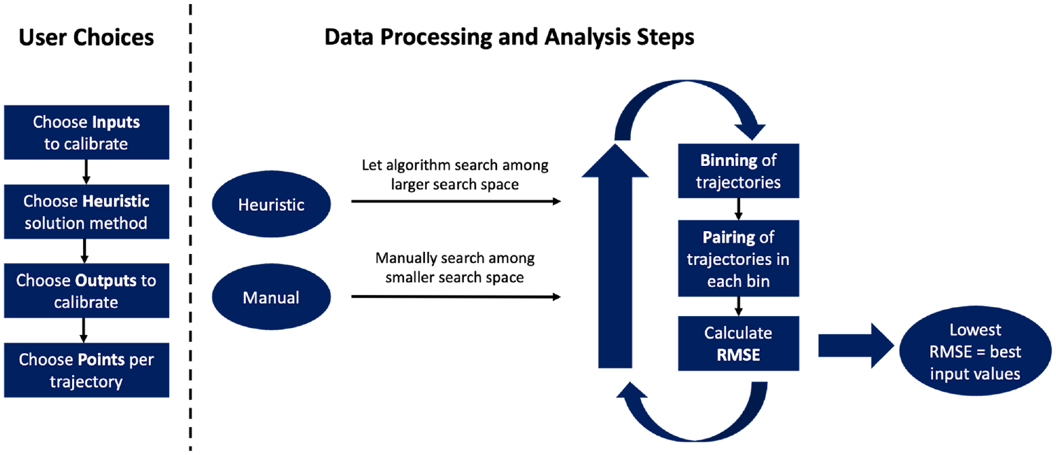
Proposed seven-step trajectory-based calibration method.

Step 1: Inputs

As mentioned in the first section, the developed trajectory-based driver behavior calibration framework is model agnostic: that is, the analyst is free to select the car-following and lane-changing model they wish to calibrate. Step 1—inputs—seeks to answer the following questions: which calibration parameters does the analyst wish to calibrate, and how should the analyst limit the search space for each parameter? This step was motivated by the findings of Punzo et al. ( 14 ), who noted that there may exist a simplified version of car-following models that only calibrates the most sensitive calibration parameters (leaving the remaining parameters at default values) without sacrificing significant predictive power. This makes the decision of which inputs to calibrate a tradeoff decision. If a user chooses to calibrate only one car-following parameter, the task would be relatively computationally easy. However, the resulting calibrated model might not be robust enough to trust under various conditions. By contrast, if a user chose to calibrate 10 parameters, this would likely produce a more robust model, but it might be impractical to evaluate the excessive number of combinations. The selection of calibration parameters and search spaces could be informed by the literature, guidance from state agencies, sensitivity analyses, or engineering judgment.

Accordingly, the authors selected a subset of the available car-following and lane-changing parameters in the VISSIM and AIMSUN simulation software for their calibration experiments. In addition, the team selected a relatively small number of candidate values for each selected parameter to limit the number of overall candidate solutions. The team used their experience with the microsimulation tools, along with available tool-specific guidance in the literature ( 16 – 18 ), to determine which input parameters and candidate values to use in the experiments.

For the VISSIM experiments, the team decided to calibrate three car-following and four lane-changing parameters: CC1 (spacing time), CC4 (negative following threshold), CC5 (positive following threshold), deceleration reduction distance (own), deceleration reduction distance (trailing), accepted deceleration (trailing vehicle), and safety distance reduction factor. The literature recommended calibrating CC0 (jam spacing). However, the dataset collected for this project lacked sufficient stop-and-go traffic conditions to allow the team to calibrate this parameter. To make the problem more practical, the team identified ranges of values to consider for each calibration parameter. The values considered for the Wiedemann 99 car-following model are as follows.

CC1: 0.7, 0.8, and 0.9 s.

CC4: −0.25 and −0.35.

CC5 was set equal to −CC4 (e.g., if CC4 = −0.25, then CC5 = 0.25).

The following lane-change model parameters and candidate values were selected for calibration.

Deceleration reduction distance (own): 50, 100, and 200 ft.

Deceleration reduction distance (trailing) was set equal to the value above.

Accepted deceleration (trailing vehicle): −1.64, −3.28, and −6.27 ft/s².

Safety distance reduction factor: 0.2, 0.4, and 0.6.

For the AIMSUN experiments, the team decided to calibrate three car-following and two lane-changing parameters: reaction time, car-following aggressiveness, sensitivity factor deviation, lane-changing cooperation, and lane-changing aggressiveness. To make the problem more practical, the team identified ranges of values to consider for each calibration parameter based on their previous modeling experience. The values considered for the Gipps car-following model ( 19 ) are as follows.

Reaction time: 0.85, 0.90, 0.95, 1.00, 1.05, and 1.10 s.

Car-following aggressiveness: 0.0, −0.1, −0.2, −0.3, −0.4, and −0.5.

Sensitivity factor deviation: 0.00, 0.05, and 0.10.

The following lane-change model parameters and candidate values were selected for calibration.

Lane-changing cooperation: 50, 60, 70, 80, 90, and 100.

Lane-changing aggressiveness: 0, 10, 20, and 30.

The remaining parameter values were kept at their default values.

The combinations of the selected parameters and parameter search spaces led to 162 candidate solutions for VISSIM and 156 candidate solutions for AIMSUN.

Although VISSIM and AIMSUN were selected by the research team for this experiment, the research team stresses that the value of this calibration framework is that it is fully customizable at every step. Thus, analysts can use the trajectory calibration methodology with other driver behavior algorithms (e.g., SUMO, TransModeler). Moreover, analysts can use different calibration parameters for the same models in their calibration (e.g., CC0 [standstill distance], desired speed).

Step 2: Heuristics

The second step in the proposed method is to choose which search method to use for identifying the best set of calibration parameter coefficients. The search methods considered may be some form of exhaustive search algorithm or heuristic method. Heuristic methods contain special logic to automatically eliminate many combinations of values unlikely to be optimal (e.g., the genetic algorithm). Heuristics may be valuable when the number of calibration parameters and the size of search spaces are larger, resulting in a higher number of possible solutions. Without heuristics, it is necessary to explicitly evaluate all input parameter value combinations through exhaustive enumeration or brute-force searching. Like Step 1, the proposed trajectory calibration method places no restriction on the search method, as no one-size-fits-all search method exists.

As discussed in Step 1, the research team decided to limit the number of calibrated parameters and the search spaces such that there were only 162 candidate solutions for VISSIM and 156 candidate solutions for AIMSUN. Thus, for the case studies presented in this paper, the authors chose to use directed brute-force (DBF) searching ( 20 ).

The above discussion illustrates a potential interdependence between Steps 1 and 2 of the proposed calibration process. In other words, a user’s choice of inputs to calibrate (Step 1) might be influenced by which search methods the user wishes to implement (Step 2). Conversely, a user’s choice of search method (Step 2) might be influenced by what input parameters the user needs or wants to calibrate (Step 1), because many inputs usually cannot be calibrated by exhaustive enumeration. These choices might be affected by other considerations, such as the size of the traffic network, the number of time periods to simulate, the speed of the computer, and the speed of the simulation product. These factors affect the amount of time needed per simulation run, which in turn affects the amount of time needed for calibration. As an example, suppose the user has selected a car-following and lane-changing model with a total of six parameters; assume that the user has identified five candidate values for each of the six parameters. In this case, the number of possible solutions is 5⁶ = 15,625. As such, a heuristic search method (e.g., genetic algorithm, random search, gradient-based methods) will be necessary to limit the search space to the most likely optimal values to avoid performing 15,625 different simulations. By contrast, suppose the user is willing to restrict calibration to the two most sensitive parameters, with five candidate values for each parameter. In this case, the search space is 5² = 25 possible parameter sets. In this scenario, the analyst may consider an exhaustive search method or a heuristic. The trajectory calibration framework developed in this paper is flexible enough to allow the analyst to choose to use an exhaustive numeration method (e.g., DBF) or a heuristic (e.g., genetic algorithm, random search, gradient-based methods) based on their calibration problem.

Step 3: Outputs

The third step of the proposed method is to choose output performance measure(s) on which the analyst will evaluate the effectiveness of the calibration procedure by comparing the simulated output performance measure(s) against observed output performance measure(s). The analyst may select one or more performance measure(s) for comparison. The output performance measure selection could be motivated by the literature, state simulation modeling guidance, sensitivity analysis, or engineering judgment.

For a purely trajectory-based calibration, the authors suggest using headways for car-following dynamics and lane identification (ID) numbers for lane-changing dynamics throughout the entire trajectory. This decision was motivated by the literature review, where several papers noted that the use of headways more effectively captures car-following dynamics throughout a trajectory. In the absence of similar literature on how to capture lane-changing effects, the team hypothesized that lane ID numbers could be an effective output performance measure. The use of lane ID numbers as a performance measure allows the calibration method to assess if the simulated and observed vehicle are in the same lane at the same point, both temporally and spatially, in the trajectory. In addition, both headways and lane ID numbers were also readily available within the proposed trajectory data format ( 4 ).

If multiple performance measures of interest are identified, the user will need to specify the relative weighting of these performance measures to the optimization problem (e.g., are car-following and lane-changing equally important or is one performance measure more important than the other?). Step 7 of the method will demonstrate how these output measures and relative weightings affect calculations within the calibration process.

Step 4: Points

The fourth step in the proposed method enables the analyst to decide how many times the procedure compares the predicted performance measure to the performance measure observed in the field. In Figure 2, the trajectories of two vehicles (e.g., a simulated vehicle and an observed vehicle) are compared to each other 27 times. If well calibrated, the trajectories of the two vehicles should be nearly identical, because Step 8 seeks to minimize the RMSE between the simulated and observed trajectories. The trajectories in Figure 2 would not be considered well calibrated because they are substantially different.

Figure 2.

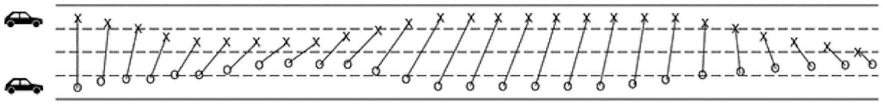
Comparison of full-set trajectories.

The decision of how often to compare the predicted performance measure to the performance measure observed in the field could be based on a desired number of points (e.g., 27 points per trajectory, as shown in Figure 2), time (e.g., every 2 s) or space (e.g., every 50 ft). There is a tradeoff with this decision. More frequently comparing the trajectories (i.e., a higher number of points) will likely improve model robustness, but at the expense of increased run times for analyses; conversely, if trajectories are compared less frequently, this will reduce the required run time, but may also reduce the effectiveness of the calibration process. The analyst is free to choose the number of times they wish for observed and simulated performance measures to be compared. This decision may be informed by the literature, early sensitivity analysis, or engineering judgment.

The research team used 2-s intervals (for VISSIM) and 50-m intervals (for AIMSUN) between points for the case study experiments featured in this paper. In the absence of guidance in the literature, the researchers hypothesized that interval durations near average driver reaction times might appropriately balance the tradeoff decision in Step 4.

Step 5: Binning

There is significant evidence in the literature of inter- and intra-driver heterogeneity in trajectory level data as a function of driver attributes, driver aggression, level of congestion, operational condition, weather conditions, lane type, and leading vehicle type. Thus, one of the challenges with the trajectory calibration process is ensuring that sufficiently similar trajectories are compared (e.g., it would be inappropriate to compare an aggressive driver’s trajectory to a defensive driver’s trajectory, just as it would be inappropriate to compare a trajectory collected in congested conditions to a trajectory collected in uncongested conditions).

Thus, the fifth step in the proposed method involves the binning of trajectories (both simulated and field-observed) into specific groups to enable the method to compare sufficiently similar trajectories. The binning process seeks to identify groups of drivers that are likely to behave similarly, minimizing the heterogeneity within the group ( 21 ). This is another decision with tradeoffs for the analyst to consider: increasing the number of bins for the data will likely reduce the heterogeneity within the binned data, but will increase the computational time of the calibration procedure. The analyst is free to choose the types of bins based on their data, but must ensure that at the end of the binning process there is a sufficient number of similar trajectories for sampling during the pairing step (Step 6). Sample bin categories include, but are not limited to, lane type (e.g., general purpose, high-occupancy toll), vehicle type (e.g., passenger vehicle, heavy vehicle, motorcycle, etc.), driver type (e.g., aggressive, conservative), weather (e.g., rain, clear), and operational conditions (e.g., work zone, level of congestion, lane width).

Given the datasets available for this research, the selected bins included origin and destination lanes, vehicle type, and driver type. The team divided each origin lane and on-ramp into separate bins, producing four separate bins (three general purpose lanes and one on-ramp). Within each of these bins, the team further divided the data by destination lane type: either general purpose lane or off-ramp. This produced a total of eight bins. The team next binned the data by driver type: aggressive or conservative. Within each of the eight bins (separated by origin and destination lane), drivers maintaining a below median time headways were classified into the aggressive driver bin, while above the median time headways were classified into the conservative driver bin. Finally, given the low number of heavy vehicles and motorcycles in the underlying data, those vehicle types were filtered out of each of the bins such that only passenger cars were included. This resulted in a total of 16 bins for the case studies documented in this paper.

Once the bins are finalized, the data should be separated into calibration and validation data. The team then set aside 20% of the trajectories in each bin for subsequent validation experiments. This allowed the team to validate the robustness of the calibration process on data that were similar, but were not used for calibration.

Step 6: Pairing

After the analyst bins the trajectories, the calibration method pairs a simulated trajectory to an observed trajectory within the same data bin from Step 5 (e.g., origin lane 1, general purpose lane destination, aggressive driver, passenger car). Pairing vehicles that entered at similar times may help calibration effectiveness, because driver behaviors are sensitive to traffic congestion levels, which change over time ( 22 , 23 ). Thus, the authors recommend pairing trajectories based on when they enter the study area; this could be a spatial or temporal threshold.

In the pairing step, the analysis is required to make two decisions, as follows.

Given an observed trajectory, which simulated trajectory should it be compared against?

How many trajectories in a bin should be compared?

For the first decision, the research team used timestamp-based pairing for the case study experiments featured in this paper. The team paired a field-observed vehicle with any simulated vehicle entering the study area within 4 s of another. In the case that multiple trajectories qualified for pairing, one trajectory was randomly selected. It is important to note that this threshold may be dataset specific. The 4-s threshold was found to work well on the data available to the team, but may need to be identified through sensitivity analysis or engineering judgment for different datasets.

The binning process required in Step 6 is repeated until each observed trajectory is paired with a simulated trajectory in the same bin. This is where decision 2 is required. The number of trajectories compared in each bin requires a tradeoff: if many paired trajectories are considered, this may increase the overall accuracy of the calibration process; however, this may increase the amount of time required for calibration. Thus, the analyst may wish to set a maximum number of trajectories. The research team applied a maximum of 25 paired trajectories per bin for its own experiments. It should be noted that the selection of 25 paired trajectories for these case studies was arbitrary and would benefit from sensitivity analyses in future studies.

This process can be automated through scripting using the following logic.

For each bin:

order field-observed vehicles according to their entry into the study area;

repeat until either the simulated or observed data bin is empty.

Select a field-observed vehicle.

If a simulated vehicle entered the study area within 4 s of the observed vehicle’s entry time, pair these two trajectories and remove them from the pool of unpaired trajectories.

Step 7: RMSE

After the analyst pairs the trajectories, Step 7 quantifies the similarity between the observed and simulated trajectories. The objective of the calibration process is to minimize the difference between the observed and simulated trajectories. As discussed in the Literature Review section, the RMSE has been found to work well as the goodness-of-fit function for driver behavior calibration and was adopted as part of this process. For the vehicle trajectory-based calibration, the RMSE needed to reflect the similarity of the trajectories for both car following (i.e., headways) and lane changing (i.e., lane ID number). Thus, the team needed to normalize both performance measures such that they could be combined into a single dimensionless value, even though they possess fundamentally different units of measurement.

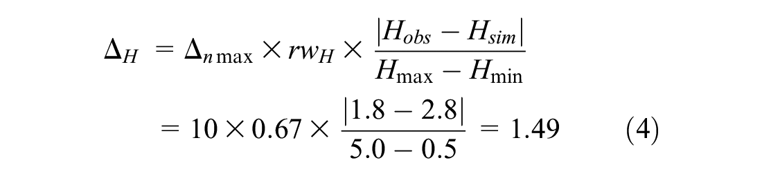
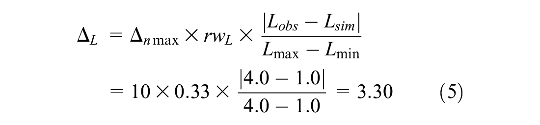
The first decision that analysts need to be make is to decide the relative importance of car following versus lane changing (e.g., a relative weighting of 75–25 would mean the analyst wants car following to be three times as influential as lane changing). In the absence of research on this topic, the research team decided to treat car following and lane changing as equally important. Secondly, the analyst should define the acceptable range limits for each performance metric that needs to be normalized based on their data sample. Thirdly, the analyst should use Equation 1 to compute the similarity of each trajectory point for each performance metric (Equation 1 shows the equation for headways, but an analogous equation can be derived for lane ID number). Equation 1 gives the difference between the observed and simulated headway at a specific point in the trajectory. Next, the total difference, or total delta, is found by summing the delta of all selected performance measures (Equation 2) for each trajectory pair. Finally, after obtaining the normalized total delta values for all trajectory pairs in each bin, Equation 3 computes the normalized RMSE:

Δ_{H} = Δ_{n max} \times r w_{H} \times \frac{| H_{obs} - H_{sim} |}{H_{max} - H_{min}}

(1)

where Δ_H is the delta headway, Δ_nmax is the normalized maximum delta value, rw_H is the relative weighting for headways, H_obs is the field-observed headway (seconds), H_sim is the headway in the simulation (seconds), H_max is the acceptable maximum headway (seconds), and H_min is the acceptable minimum headway (seconds):

Δ_{tot} = Δ_{H} + Δ_{L}

(2)

where Δ_tot is the total delta for one paired trajectory and Δ_L is the delta lane ID number:

RMSE = \sqrt{\frac{\sum_{T} {Δ_{tot}}^{2}}{T}}

(3)

where T is the total number of trajectory pairs across all bins and Δ_tot is the total delta for one paired trajectory point.

At the conclusion of this step, there is a singular RMSE value for each candidate combination of input parameter values simulated. The lowest RMSE value then indicates which set of input parameter coefficients allow the simulation to best replicate field conditions. A RMSE value of 0 would indicate a perfectly calibrated model. Ideally, analysts should execute multiple random number seed replications to obtain a more statistically reliable RMSE for each combination of input values.

To demonstrate the normalization calculation, let us assume a 67–33 weighting, indicating that car-following is twice as important as lane-changing. This may be expressed as a relative weighting for headways (i.e., rw_H = 0.67) and a relative weighting for lanes (i.e., rw_L = 0.33). For Equation 1, the analyst must next identify the minimum and maximum values for the headway and lane number. This will be specific to the collected data. For the drone-collected trajectory data, the team identified a range of 0.5–5.0 for headways (i.e., H_min = 0.5; H_max = 5.0) and a range of 1–4 for lane ID number (i.e., L_min = 1.0, L_max = 4.0 for a four-lane roadway). Finally, for Equation 1, the analyst should define the normalized maximum delta (Δ_nmax). Although any value can be used here, a Δ_nmax of 10 will be assumed for the sake of demonstration. In other words, a Δ_nmax value of 0 would indicate a perfectly calibrated paired trajectory point, whereas a Δ_nmax of 10 would indicate a maximally unrealistic trajectory point. Finally, let us assume that at one of the comparison points (Step 4) the observed headway is 1.8 s and the simulated headway is 2.8 s. In addition, assume the vehicle is observed to be in lane 4 in the field and lane 1 in the simulation. The sample calculation for the vehicle at that point in their trajectory is as follows:

\begin{matrix} Δ_{H} \end{matrix} = Δ_{n max} \times r w_{H} \times \frac{| H_{obs} - H_{sim} |}{H_{max} - H_{min}} = 10 \times 0.67 \times \frac{| 1.8 - 2.8 |}{5.0 - 0.5} = 1.49

(4)

\begin{matrix} Δ_{L} \end{matrix} = Δ_{n max} \times r w_{L} \times \frac{| L_{obs} - L_{sim} |}{L_{max} - L_{min}} = 10 \times 0.33 \times \frac{| 4.0 - 1.0 |}{4.0 - 1.0} = 3.30

(5)

Δ_{tot} = Δ_{H} + Δ_{L} = 1.49 + 3.30 = 4.79

(6)

To compute the total RMSE for this particular simulated–observed vehicle pair, this calculation should be completed at every point along the trajectory. To compute the total RMSE for this particular set of calibration parameters, this calculation should be competed for all simulated–observed vehicle pairs at all points along their trajectories, as shown in Equation 3.

Trajectory Calibration Summary

The proposed seven-step trajectory calibration procedure computes a single RMSE for each combination of input parameter values. The combination of values producing the lowest RMSE is selected as the best solution, because this set of values produces simulated trajectories that are most similar to the observed trajectories. At a high level, the process involves four user choices (Steps 1–4) and three data processing steps (Steps 5–7). Figure 1 illustrates these seven steps. Recall that during Step 6, a portion of the trajectory data (i.e., 20% from each bin) is set aside specifically for validation. Both datasets (i.e., calibration and validation) should have a similar proportion of trajectories in each bin. The analyst can subsequently use the validation dataset to assess the predictive power of their calibrated model.

The trajectory calibration framework is fully customizable. However, to demonstrate the performance of the calibration framework, the research team conducted a series of experiments in two different commercial microsimulation software packages. The following summarizes the research team’s decisions in operationalizing the trajectory calibration framework (Figure 1) for the experiments detailed in the Results and Discussions section.

Step 1, inputs.

VISSIM experiments.

CC1: 0.7, 0.8, and 0.9 s.

CC4: −0.25 and −0.35.

CC5 was set equal to −CC4 (e.g., if CC4 = −0.25, then CC5 = 0.25).

Deceleration reduction distance (own): 50, 100, and 200 ft.

Deceleration reduction distance (trailing) was set equal to the value above.

Accepted deceleration (trailing vehicle): −1.64, −3.28, and −6.27 ft/s².

Safety distance reduction factor: 0.2, 0.4, and 0.6.

All other car-following and lane-changing parameters left at default values.

AIMSUM experiments.

Reaction time: 0.85, 0.90, 0.95, 1.00, 1.05, and 1.10 s.

Car-following aggressiveness: 0.0, −0.1, −0.2, −0.3, −0.4, −0.5.

Sensitivity factor deviation: 0.00, 0.05, and 0.10.

Lane-changing cooperation: 50, 60, 70, 80, 90, and 100.

Lane-changing aggressiveness: 0, 10, 20, and 30.

All other car-following and lane-changing parameters left at default values.

Step 2, heuristic: DBF method.

Step 3, outputs.

Car following: headway.

Lane changing: lane ID number.

Step 4, points.

VISSIM experiments: 2-s intervals.

AIMSUN experiments: 50-m intervals.

Step 5, binning.

Lane type (origin [general purpose, on-ramp], destination [general purpose, off-ramp]).

Vehicle type (passenger car).

Driver type (aggressive, conservative).

Step 6, pairing.

Pair simulated and observed vehicles entering network within 4 s of one another.

25 paired trajectories per unique bin.

Split data: 80% calibration, 20% validation.

Step 7, RMSE.

Car following is considered equally important to lane changing (i.e., 50/50 relative weighting split).

Traditional Calibration Method

As mentioned in the introduction, the project scope required calibrating four microsimulation models according to both traditional and trajectory-based methods to assess the advantages and disadvantages of the newly developed trajectory method. For this purpose, the researchers endeavored to perform traditional calibration in a manner similar to the trajectory-based calibration. The motivation for this was to facilitate comparisons of driver behavior calibration, which was a key project objective. Moreover, applying certain systematic aspects of the trajectory methodology toward traditional calibration could conceivably produce better outcomes than can be achieved in practice, where input parameters are typically modified in a trial-and-error fashion. The authors consider this method to be traditional because it uses data that is traditionally used to calibrate microsimulation models in practice (e.g., average lane speed and throughput).

The adopted traditional calibration method started with the benchmark model (i.e., calibrated demands, default driver behavior parameters), as described earlier in the Methodology section. The remainder of this section describes how the research team adjusted Steps 1–7 to complete the traditional calibration.

Step 1 (inputs) of the traditional calibration methodology was identical to the trajectory-based calibration methodology. That is, the traditional calibration method selected the same input parameters and parameter search spaces as were selected for the trajectory-based methodology. The motivation behind this decision is that the car-following and lane-changing calibration parameters are the same, whether one is using traditional data (and calibration methods) or trajectory data (and calibration methods).

Step 2 (heuristic) of the traditional calibration methodology was also identical to the trajectory-based calibration method. The traditional calibration methodology used the DBF search method to exhaustively simulate each possible combination of input values. The decision to keep Steps 1 and 2 of the traditional calibration methodology consistent with the trajectory calibration methodology significantly reduced the computation time for the case studies, because the same 162 candidate solutions for VISSIM and 156 candidate solutions for AIMSUN were used for traditional calibration without the need for additional simulations or datasets.

Step 3 (outputs) of the traditional calibration method is where the methodologies are most different. Step 3 defines how the optimal parameter set was identified for the traditional calibration method. For a more traditional calibration of a freeway microsimulation model, these outputs are typically aggregate performance measures, such as segment or lane-by-lane speed, throughput, density, and bottleneck duration ( 14 ). The selected average segment speeds and throughput are used as the traditional output performance metrics to compare between the simulated and observed data (instead of headways and lane numbers, which were used for trajectory calibration).

Steps 4–6 are unique to the trajectory-based method and were not used as part of the macroscopic calibration method.

For Step 7 (RMSE), the team selected the RMSE as the goodness-of-fit measure between simulated and observed macroscopic performance measures (i.e., throughput [counts] and speed). For normalization, the team used the highest and lowest observed speeds and throughputs as the ranges. Moreover, the team assumed a 50–50 weighting for throughputs and speeds.

This altered approach to Steps 1–3 and 7 meant that for every unique combination of input parameter values, the research team could calculate both a traditional and a trajectory-based RMSE. The team identified the parameter set corresponding with the lowest traditional RMSE value as the optimal set of calibration parameters for the traditionally calibrated model; analogously, the parameter set corresponding with the lowest trajectory RMSE value was identified as the optimal set of calibration parameters for the trajectory-based calibrated model.

The research team obtained macroscopic field measurements through traditional methods, such as radar and floating car runs, simultaneously while the aerial data collection companies collected the video footage that was processed to obtain the trajectory data. In this manner, the field-observed throughputs, speeds, headways, and lane numbers represent the same traffic conditions, thus facilitating direct comparison of traditional and trajectory-based calibration.

Hybrid Calibration Method

A hybrid calibration objective function that involves both trajectories and traditional measures is also possible, and was explored as part of this research. This method enables an analyst to calibrate a model considering both traditional and trajectory performance measures. To conduct a hybrid calibration, the user may either choose another relative weighting (i.e., the relative importance of trajectories versus traditional measures) or perform multiple sequential calibrations (i.e., trajectory calibration after traditional calibration). For these case studies, the authors chose the former. Similar to the relative weighting of two different traditional (importance of lane speeds versus throughput) and trajectory (importance of headways versus lane numbers) performance measures, a hybrid calibration allows the analyst to assign the relative importance of traditional performance measures versus trajectory performance measures.

To complete a hybrid calibration, the analyst should first independently calculate the normalized trajectory and traditional RMSE using the same defined normalized maximum value of a variable (Δ_nmax). Next, the analyst chooses the relative importance of trajectory versus traditional performance measures. For example, a relative weighting of 67–33 would mean the analyst wants trajectory measures to be twice as influential as traditional (macroscopic) measures within the calibration process. This may be expressed as a relative weighting for trajectory measures (i.e., rw_TRAJ = 0.67) and a relative weighting for traditional measures (i.e., rw_TRAD = 0.33). These relative weights should sum to 1.0. Finally, the analyst multiplies the trajectory RMSE by rw_TRAJ to obtain an adjusted trajectory RMSE, multiplies the traditional RMSE by rw_TRAD to obtain an adjusted traditional RMSE, and adds together the adjusted trajectory and traditional RMSEs to obtain a hybrid RMSE. At the conclusion of this step, there is a singular RMSE value for each candidate combination of input parameter values simulated. The lowest RMSE value then indicates which input parameter values allow the simulation to best replicate field conditions in a way that reflects the chosen relative weightings.

Experimental Design

This section describes the calibration and validation experimental results for the four chosen sites: I-270 in Maryland, I-15 in California, I-75 in Florida, and I-95 in Virginia. The research team collected video data via drones at all sites except I-75, where the team collected video data by helicopter over a continuous 1.2-mi section. The team analyzed three 800-ft (maximum drone coverage) sections of I-95 and I-270. At the I-15 site, the team analyzed four discrete sections with lengths of 1250, 1045, 545, and 440 ft. Given the spatial limitations of data collected via drones, the team chose discrete data collection locations according to key locations of queue buildup and dissipation identified using archived data from the National Performance Management Research Data Set. The team then extracted vehicle trajectories from the camera footage using a post-processor tool ( 24 ). This tool produced numerical vehicle trajectories for each vehicle observed in a format similar to the NGSIM data format, including useful data such as vehicle ID, vehicle class, speed, acceleration, and lane number. For additional details about the selection of data collection sites and the process used to extract numerical trajectories from video data, please see Hale et al. ( 4 ).

After obtaining the vehicle trajectories, the team calibrated the I-95, I-75, and I-270 VISSIM models using both the traditional and the trajectory calibration methods, as described in the Methodology section. In addition, the team calibrated the I-15 model using both the traditional and trajectory calibration methods in AIMSUN. By using two different commercial software solutions, this demonstrates that the trajectory calibration method is software agnostic and can be used regardless of the analyst’s choice for the microsimulation software. For all four simulation networks, the team set driver behavior input parameters to their default values before calibration and calibrated demands before calibrating driver behavior parameters. The team used 15-min initialization periods before all calibration and validation runs.

Results and Discussion

Figure 3 provides the RMSE results of the benchmark calibration (demand calibrated, default driver behavior parameters), traditional calibration (weight = 0), trajectory calibration (weight = 1), and three hybrid calibrations (weight = 0.25, traditional calibration thrice as important as trajectory calibration; weight = 0.5, traditional calibration and trajectory calibration equally important; weight = 0.75, trajectory calibration thrice as important as traditional calibration) for the I-95 (Figure 3a), I-75 (Figure 3b), I-270 (Figure 3c), and I-15 (Figure 3d) sites. In these bar charts, only the best solution (i.e., the lowest RMSE out of all candidate solutions) is shown for each weight, with a box-and-whisker notation to indicate the range of 10 random number seed outcomes per candidate.

Figure 3.

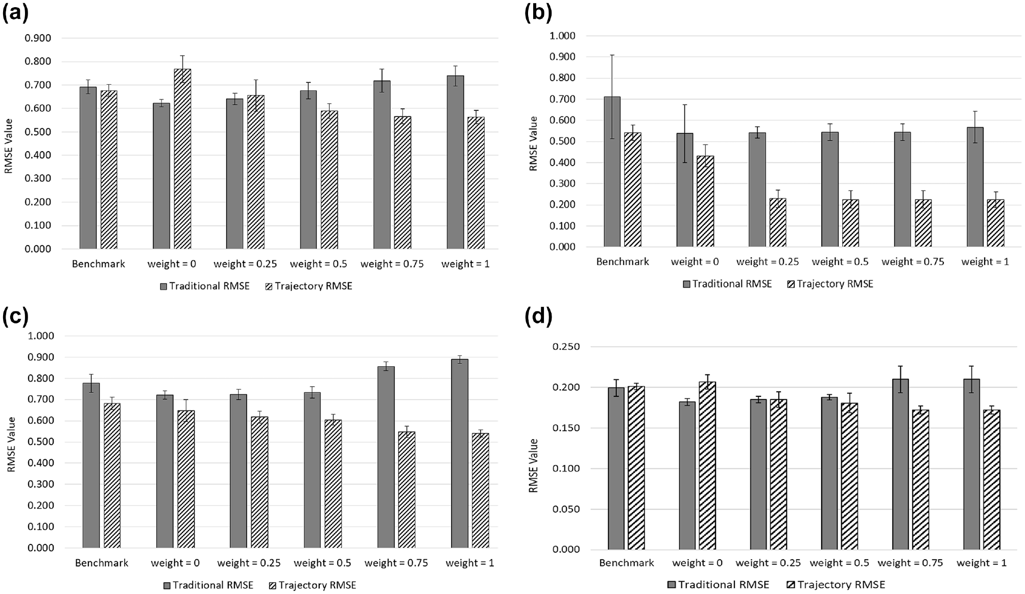
Calibration results for (a) I-95, (b) I-75, (c) I-270, and (d) I-15.

The calibration results appeared to confirm suspicions held by the research team: if trajectories are not included in the calibration process, simulated trajectories may not be very realistic, even if aggregate measures have good agreement with those observed in the field. For the I-95 and I-15 networks shown in Figure 3, a and d , the traditional calibration methodology (weight = 0) improved the estimate of the traditional RMSE (i.e., average lane speed and throughput) compared to the benchmark model, where the driver behavior parameters were not calibrated. However, the trajectories (i.e., headways and lane ID numbers) produced by the traditional calibration methodology were less accurate than if default parameters had been used. For these same networks, the trajectory-based calibration methodology (weight = 1) improved the trajectory RMSE compared to the benchmark model and the traditional calibration model, indicating that the vehicles’ lane assignment and headways better match what was observed in the real-world data. However, this methodology produced a worse traditional RMSE than the benchmark model and traditional calibration method, indicating that the lane-specific speed and throughput do not match the field data. This suggests that the type of data used for calibration (e.g., trajectories or macroscopic performance measures) influences which outputs the model will be able to better capture, and that the analyst needs to be aware of these tradeoffs (i.e., is it more importance to have accurate vehicle trajectories [e.g., headways, lane IDs] or traffic flow [e.g., throughput, speed]?).

The most substantial trajectory calibration improvements were observed with the I-75 model, which is the only site that collected data via helicopter, producing significantly longer trajectories. For the I-75 network shown in Figure 3b, the trajectory-based calibration methodology (weight = 1) improved the trajectory RMSE significantly compared to the benchmark model and the traditionally calibrated model. Moreover, this model performed equivalently well at producing lane-specific speed and throughputs (traditional RMSE) compared to the traditionally calibrated model. In this case, there was not a tradeoff between the accuracy of the traditional RMSE and the trajectory RMSE as a function of input data. The research team hypothesizes that the longer trajectories extracted from the helicopter data contributed to the improvement in modeling results.

The effect of pure trajectory calibration (weight = 1) on the traditional measures was inconsistent across the four case studies. At the I-75 site, trajectory-based calibration made the traditional measures more accurate. However, at other sites, trajectory-based calibration resulted in a more accurate trajectory RMSE, but a less accurate traditional RMSE; that is, by calibrating the models only considering headways and lane ID numbers, the observed and measured throughputs and speeds were somewhat less accurate. These results suggest that it may be important to consider both macroscopic properties of traffic flow (e.g., throughput and speed) and vehicle trajectories (e.g., headways and lane ID numbers) in the calibration process to achieve a model whose outputs are realistic across as many categories as possible.

Following calibration, the research team then evaluated the calibrated models according to the validation data, which was omitted from the calibration process (removed during Step 5 before the pairing of simulated and observed trajectories). Figure 4 graphs the resulting traditional and trajectory RMSE values for the I-95 (a), I-75 (b), I-270 (c), and I-15 (d) case studies. The trends of the traditional RMSE versus the trajectory RMSE are consistent across the calibration data (Figure 3, a–d) and the validation data (Figure 4, a–d). This indicates that the trajectory calibration method is able to capture generalizable trends in driver behavior without overfitting to the calibration data sample. These results provide further evidence that the trajectory-calibrated models provide more realistic trajectories than the benchmark or traditionally calibrated models. Figures 3, a–d, and 4, a–d, suggest that there is no one-size-fits-all approach to calibration: models calibrated with macroscopic performance measures produce results that more accurately depict the macroscopic characteristics of traffic flow (e.g., throughput, speed), while models calibrated with trajectories more accurately capture individual vehicle movement (e.g., headways, lane ID number). However, there does exist a hybrid approach to modeling, which uses both macroscopic performance measures and vehicle trajectories in the calibration process. This approach balances the tradeoff between accurately capturing the vehicle trajectories and the characteristics of traffic flow.

Figure 4.

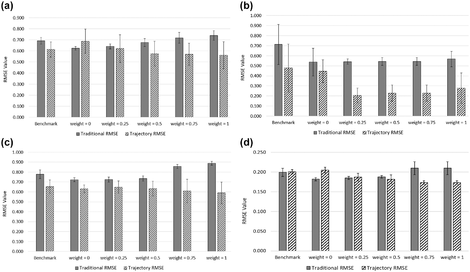
Validation results for (a) I-95, (b) I-75, (c) I-270, and (d) I-15.

Analysis of Pure Trajectory-Based and Traditional Calibration

Table 1 focuses on the potential benefits of a pure trajectory-based calibration (i.e., weight = 1), relative to a pure traditional calibration (i.e., weight = 0) or a benchmark model (calibrated demands, uncalibrated driver behavior), with regard to trajectory accuracy and realism (RMSE_trajectory) using the calibration data as the test data (corresponding with Figure 3, a–d). The first column is the difference between the RMSE_trajectory of the traditional calibration (weight = 0) relative to the RMSE_trajectory of the benchmark model. This implies that traditional calibration (i.e., minimizing the difference between the simulated and observed lane-specific throughput and speed) does not reliably improve the realism of vehicle trajectories compared to the benchmark model. Interestingly, for two of the four models, the benchmark model (default driving behavior parameters) produced trajectories that better matched field data compared to the model calibrated using lane-specific throughput and speed measurements. The second column represents the difference between the RMSE_trajectory of the trajectory calibration (weight = 1) relative to the RMSE_trajectory of the benchmark model. The second column implies that pure trajectory-based calibration (i.e., minimizing the difference between the observed and simulated headways and lane ID number) produces large improvements in trajectory accuracy compared to the benchmark model. The third column is the difference between the RMSE_trajectory of the trajectory-based calibration method (weight = 1) and the traditional calibration method (weight = 0). The third column highlights the sizeable benefit to trajectory accuracy (RMSE_trajectory) when performing trajectory-based calibration (weight = 1) instead of traditional calibration (weight = 0).

Table 1.

Impacts of Calibration on Trajectories From the Calibration Dataset

	Traditional (%)	Trajectory (%)	Benefit (%)
Interstate 95	−13	+17	+30
Interstate 75	+20	+59	+39
Interstate 270	+5	+21	+16
Interstate 15	−3	+14	+17

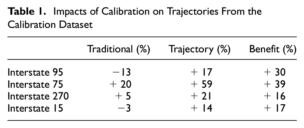
Table 2 reveals a corresponding set of results according to the validation dataset, which is data that were not used for calibration (set aside during Step 5, binning). The first column of results implies that traditional calibration (i.e., minimizing the difference between the simulated and observed throughput and speed) has a mixed impact on the realism of vehicle trajectories (RMSE_trajectory) relative to the benchmark model. This provides further evidence that traditional calibration methods cannot be trusted to produce accurately modeled vehicle trajectories. The second column implies that the trajectory-based calibration method consistently produced improved simulated trajectory predictions relative to the benchmark model. Finally, the third column highlights the potential benefits of trajectory-based calibration (weight = 1) relative to traditional calibration (weight = 0): an increase in trajectory accuracy for every case study conducted. These benefits are somewhat smaller than the Table 1 benefits. However, the research team expected this, because the validation data were not used in the calibration process. Thus, Table 2 illustrates the more-likely outcomes of using the calibrated models to make predictions, because they were evaluated against a separate validation dataset. Although the team does not have access to something comparable to a before-and-after (current-and-future) dataset, Table 2 demonstrates that the trajectory-based calibration method is able to capture generalizable trends in driver behavior that match validation data (not used in the calibration procedure) quite well, and should be explored further in future research.

Table 2.

Impacts of Calibration on Trajectories From the Validation Dataset

	Traditional (%)	Trajectory (%)	Benefit (%)
Interstate 95	−12	+9	+21
Interstate 75	+7	+42	+35
Interstate 270	+3	+10	+7
Interstate 15	+1	+14	+15

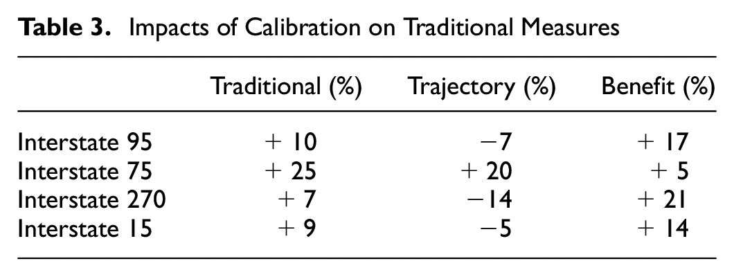
Table 3 examines the impacts of calibration on traditional measures. The first column is the difference between the RMSE_traditional of the traditional calibration (weight = 0) relative to the RMSE_traditional of the benchmark model. The first column of results implies that traditional calibration (i.e., minimizing the difference between the simulated and observed lane-specific throughput and speed) improves the realism of traditional performance measures, although the magnitude of that improvement varies across networks. The second column is the difference between the RMSE_traditional of the trajectory calibration (weight = 1) relative to the RMSE_traditional of the benchmark model. The second column implies that pure trajectory-based calibration does not reliably improve the simulated aggregate traffic flow performance measures. At two of the four sites, the reduction in accuracy was marginal. Moreover, at the site where helicopters were used for trajectory data collection, the accuracy of the aggregate traffic flow performance measures increased substantially, even though trajectory measures were not explicitly used by the calibration objective function. The third column highlights the advantage of traditional calibration (i.e., minimizing the difference between the simulated and observed throughput and speed) over trajectory-based calibration (i.e., minimizing the difference between the simulation and observed headway and lane ID numbers) with regard to aggregate traffic flow performance measure accuracy. As shown in Table 3, at the site where helicopters were used for data collection instead of drones (which produced significantly longer trajectories), the trajectory calibration method performed nearly as well as the traditional calibration method at replicating aggregate traffic flow performance measures, even though traditional measures (e.g., throughput, speed) were not considered as part of the objective function. At three of the four sites, the traditional calibration method (where the objective was to explicitly match segment-level throughput and speed) produced more accurate simulated aggregate traffic flow performance measures. However, as observed in Tables 1 and 2, this came at the significant expense of accurate individual vehicle trajectories. This motivated the study of hybrid calibrated models.

Table 3.

Impacts of Calibration on Traditional Measures

	Traditional (%)	Trajectory (%)	Benefit (%)
Interstate 95	+10	−7	+17
Interstate 75	+25	+20	+5
Interstate 270	+7	−14	+21
Interstate 15	+9	−5	+14

Analysis of the Hybrid Calibration Method

The research team developed the hybrid calibration method to enable analysts to include both trajectories and aggregated traffic flow performance metrics in the calibration process. In the absence of guidance, this section will analyze the results of the 50–50 hybrid calibrated model, which considered trajectories and aggregated traffic flow performance metrics as equally important in the calibration process.

Table 4 details the impact of the hybrid calibration method (weight = 0.5) on the accuracy of simulated trajectories (RMSE_trajectory) versus the benchmark model and the pure traditional calibrated model (weight = 0) using the calibration data as the observed data. As one can see, using both trajectories and aggregate traffic flow performance metrics in the calibration process through a unique hybrid method produces models that are much more robust and accurately simulate vehicle trajectories that match what was observed in the field data.

Table 4.

Impacts of 50–50 Hybrid Model on Trajectories From the Calibration Dataset

	Versus benchmark (%)	Versus traditionally calibrated (%)
Interstate 95	+13	+23
Interstate 75	+58	+48
Interstate 270	+11	+7
Interstate 15	+10	+13

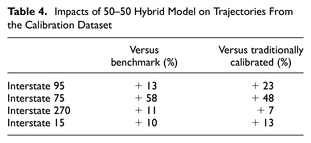
Table 5 details the impact of the hybrid calibration method (weight = 0.5) on the accuracy of simulated trajectories (RMSE_trajectory) versus the benchmark model (column 1) and the pure trajectory calibrated model (weight = 1) using the validation data as the observed data. This table provides further evidence that a hybrid approach performs much better at producing accurately simulated trajectories compared to models that were not calibrated (benchmark), or models that were calibrated only with macroscopic data. Moreover, when comparing Tables 4 and 5, one does not observe a significant decrease in accuracy despite using holdout data as the observed data; this strongly suggests that the hybrid calibration method produces models that are not overfit to the calibration data, and captures generalizable trends in driver behavior.

Table 5.

Impacts of 50–50 Hybrid Model on Trajectories From the Validation Dataset

	Versus benchmark (%)	Versus traditionally calibrated (%)
Interstate 95	+6	+16
Interstate 75	+52	+49
Interstate 270	+3	+0
Interstate 15	+9	+11

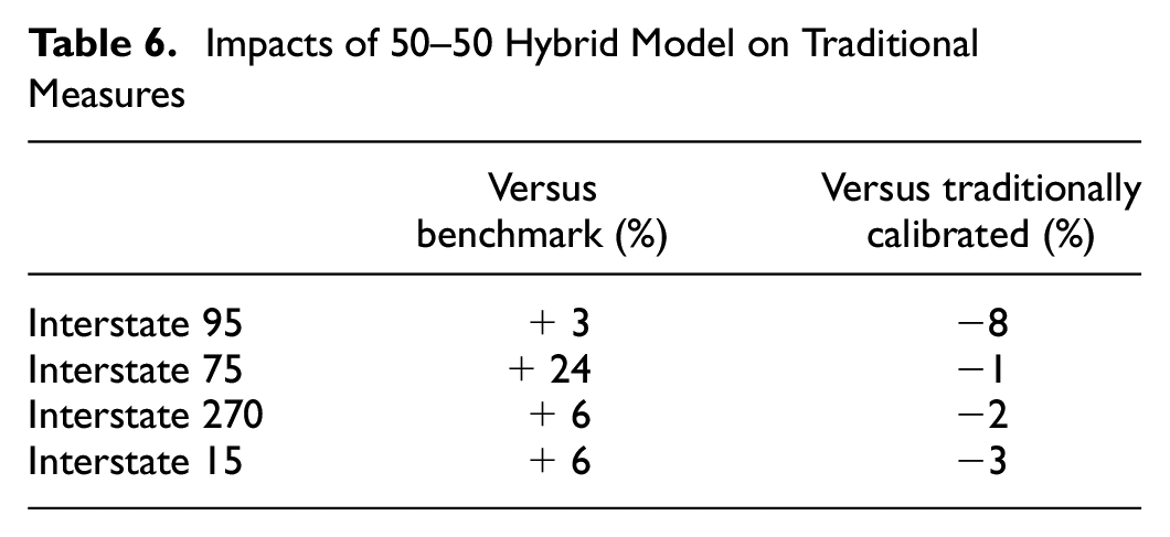
Finally, Table 6 examines the impact of the hybrid calibration method (weight = 0.5) on traditional measures (RMSE_traditional). The first column, which evaluates performance of the 50–50 hybrid calibration method relative to the benchmark model, suggests there is a modest benefit to the accuracy of aggregate traffic flow performance measures by including trajectories and lane-specific throughput and speed data as part of the calibration process. The second column evaluates performance of the 50–50 hybrid calibration method relative to the traditionally calibrated model (weight = 0). Compared to column 3 of Table 3, one observes negligible reductions in the accuracy of the simulated throughput and speed when using both trajectories and field-collected lane-specific throughput and speed as the calibration data.

Table 6.

Impacts of 50–50 Hybrid Model on Traditional Measures

	Versus benchmark (%)	Versus traditionally calibrated (%)
Interstate 95	+3	−8
Interstate 75	+24	−1
Interstate 270	+6	−2
Interstate 15	+6	−3

Thus, the authors of this paper believe that a hybrid calibration approach—using both trajectories and lane-specific throughput and speed—for the calibration of driver behavior models in microsimulation provides a substantial improvement over current best practices. This is because the hybrid calibration approach produces models whose simulated trajectories match field observations much more accurately, without sacrificing the accuracy of macroscopic traffic flow performance metrics.

Modeling Implications

Based on this documented research, the authors make the following general calibration recommendations.

The driver behavior parameters of microsimulation models should always be calibrated using best practices. This research adds to a body of literature that recognizes the importance of model calibration and suggests that default driver behavior parameters are not sufficient for capturing real-world driver behavior in microsimulation model analyses.

Moreover, when appropriate data are unavailable, the authors of this paper caution practitioners against choosing high-resolution microsimulation models when conducting modeling analysis projects. Although the visualizations produced using microsimulation models are helpful for communication, it is our professional responsibility to ensure the models are calibrated appropriately to reflect local conditions without being overfit to the data.

The authors of this paper believe that a hybrid calibration approach—using both trajectories and lane-specific throughput and speed—for the calibration of driver behavior models in microsimulation provides a substantial improvement over current best practices. The hybrid calibration approach produces models whose simulated trajectories more accurately match field observations without sacrificing the accuracy of macroscopic traffic flow performance metrics.

When calibrating driver behaviors such as car following and lane changing, it is preferable to incorporate lane-specific measures instead of segment-specific measures.

The validation experimental results highlight the importance of validation in identifying problems in the calibrated models, fixing those problems, and making the calibrated models more robust and predictive.

The longer trajectories (collected via helicopter) are more desirable than data collected via individual drones. Calibrations completed using longer trajectories (>1.2 mi) outperformed the shorter trajectories (800 ft) with regard to simulated trajectories and the simulated lane-specific throughput and speed. Moreover, the model calibrated using longer trajectories performed just as well at capturing lane-specific throughput and speed as the model calibrated using lane-specific throughput and speed. This may suggest that with longer trajectories, a purely trajectory-based calibration method may be sufficiently reliable, but future research is needed on the topic.

Conclusions

Thanks to recent improvements in data collection and processing technologies for vehicle trajectories, trajectory-based calibration of microsimulation models is now a more feasible and practical option for transportation agencies to consider. In response, this project produced a methodology that explicitly incorporates vehicle trajectories into the calibration process. Phase 1 of this project was to conduct a comprehensive data collection and data processing effort at four real-world congested freeway sites, which is documented in Hale et al. ( 4 ). The paper discusses the process of developing an innovative microsimulation model calibration method using high-resolution vehicle trajectories. The research team’s goal was to make this methodology practical and straightforward. The first four steps—inputs, heuristics, outputs, and points—are user-defined choices, whereas the last three steps—binning, pairing, and RMSE—are iterative processes that can be automated through scripting.

The experimental results imply that traditional calibration methods using traditional data sources (e.g., average lane speed, throughput) cannot be trusted to predict realistic driver behaviors (i.e., car following and lane changing), even if they are replicating traffic flow well at a macroscopic level. This has significant implications for how practitioners think about calibrating their models. Case studies conducted as part of this project suggest that the inclusion of trajectories within the calibration process improves the model’s predictions of individual vehicle movements. However, although the trajectory RMSE improved, the traditional RMSE, which captured the dissimilarity between the simulated and observed throughputs and speeds, increased. This suggests that a hybrid approach—including both traditional and trajectory measures—may be the best option to calibrate robust models able to accurately capture individual trajectories and traffic flow. Case studies demonstrate that the hybrid method does not typically identify the best (i.e., lowest) trajectory or traditional RMSE. However, the hybrid method does a much better job of balancing the need for accurate trajectories (i.e., headways, lane numbers) and macroscopic traffic performance measures (e.g., average lane speed, throughput) than either methodology that excludes the other data type (i.e., purely trajectory-based or purely traditional calibration).

The magnitude of data available for calibration also appears to make a difference in trajectory calibration success. The drone-collected trajectories were only about 800 ft in length, while the helicopter-collected trajectories were close to 1.2 mi in length. The research team tried to compensate for the limited spatial coverage of the drones by deploying multiple drones at key points of interest to capture the onset, peak, and dissipation of congestion. However, the network calibrated with helicopter trajectories achieved a lower trajectory RMSE score than other networks. Moreover, the full-trajectory calibration method using helicopter-collected trajectories better replicated the macroscopic traffic flow measures than the trajectory calibration method using drone-collected data.

As with most exploratory research, the experiments in this study raised additional questions that future research could potentially examine. Future research questions include, but are not limited to, the following.

In this study’s trajectory-based calibration experiments, the relative importance of car following and lane changing was always set to 50–50. Would the process be more robust under a different relative weighting? If so, could analysts predict optimal relative weightings as a function of traffic network conditions?

Can accurate trajectories be formed by stitching together shorter trajectories (collected by multiple drones) in a cost-effective manner?

Alternatively, can analysts obtain lengthy and accurate trajectories through probe data and successfully apply these data toward calibrating microsimulation models?

In this study’s trajectory-based calibration experiments, the research team achieved favorable results by applying 80% of the trajectory data toward calibration and 20% of the trajectory data toward validation. Would this distribution of data work well for other sites? If not, could analysts predict the appropriate distribution of data according to site characteristics, traffic characteristics, or both?

How reliable are the available data collection and data processing methods for trajectory data compared to traditional data?

What is the minimum number of sampled trajectories to reliably calibrate driver behavior models using the proposed method?

What would be the effect of calibrating multiple driver behavior models for multiple congestion regimes (e.g., below capacity, near capacity, at capacity, above capacity)?

Finally, for additional information about the drone and helicopter data collection, data processing using Video-based Intelligent Road Traffic Universal Analysis Tool (VIRTUAL), trajectory calibration methodology, traditional calibration methodology, hybrid calibration methodology, or the four experimental case studies, the authors refer the reader to the Federal Highway Administration (FHWA) published report ( 4 ).

Footnotes

Acknowledgements

The authors thank the members of the pooled fund study and the developed stakeholder group for reviewing deliverables and providing feedback throughout the study. The authors also thank the FHWA subject matter experts for their helpful ideas, insights, and guidance during the study.

Author Contributions

The authors confirm contribution to the paper as follows: study conception and design: D. Hale, R. James; data collection: D. Zhao, X. Li; analysis and interpretation of results: A. Ghiasi, F. Khalighi, D. Hale, R. James; draft manuscript preparation: D. Hale, R. James. All authors reviewed the results and approved the final version of the manuscript.

Declaration of Conflicting Interests

The author(s) declared no potential conflicts of interest with respect to the research, authorship, and/or publication of this article.

Funding

The author(s) disclosed receipt of the following financial support for the research, authorship, and/or publication of this article: This research was conducted through FHWA’s Saxton Transportation Operations Laboratory under contract DTFH6116D00030. This research was funded by the Traffic Analysis and Simulation Pooled Fund Study (TPF 5-176).

ORCID iDs

David K. Hale

Farnoush Khalighi

Xiaopeng (Shaw) Li

References

Bloomberg

Swenson

Haldors

Comparison of Simulation Models and the HCM. Presented at 82nd Annual Meeting of the Transportation Research Board, Washington, D.C., 2003.

Banks

Cook

Fredrick

Gill

Gray

Larue

Milton

, et al. Successful Approaches for the Use of Unmanned Aerial Systems by Surface Transportation Agencies. NCHRP Project 20-68A. National Cooperative Highway Research Program, Washington, D.C., 2018.

U.S. Department of Transportation. Next Generation Simulation (NGSIM) Vehicle Trajectories and Supporting Data Web Page. https://data.transportation.gov/Automobiles/Next-Generation-Simulation-NGSIM-Vehicle-Trajector/8ect-6jqj. Accessed October 29, 2019.

Hale

D. K.

Ghiasi

Zhao

Khalighi

Aycin

Trajectory Investigation for Enhanced Calibration of Microsimulation Models. FHWA Final Report. Federal Highway Administration, McLean, VA, 2021. https://doi.org/10.21949/1521658.

Shi

Zhao

Yao

Hale

D. K.

Ghiasi

Video-Based Trajectory Extraction With Deep Learning for High-Granularity Highway Simulation (HIGH-SIM). Communications in Transportation Research, Vol. 1, 2021, p. 100014. https://doi.org/10.1016/j.commtr.2021.100014.

Treiber

Kesting

Microscopic Calibration and Validation of Car-Following Models – A Systematic Approach. Procedia - Social and Behavioral Sciences, Vol. 80, 2013, pp. 922–939.

Punzo

Formisano

Torrieri

Nonstationary Kalman Filter for Estimation of Accurate and Consistent Car-Following Data. Transportation Research Record: Journal of the Transportation Research Board, 2005. 1934: 2–12.

Ciuffo

Punzo

Montanino

The Calibration of Traffic Simulation Models: Report on the Assessment of Different Goodness of Fit Measures and Optimization Algorithms. JRC Scientific Report. Publication Office of the European Union, Luxembourg, 2012.

Montanino

Ciuffo

Punzo

Calibration of Microscopic Traffic Flow Models Against Time-Series Data. Proc., 15th International IEEE Conference on Intelligent Transportation Systems, Anchorage, AK, IEEE, New York, 2012, pp. 108–114.

10.

Chu

Liu

J.-S.

Recker

A Calibration Procedure for Microscopic Traffic Simulation. UCI-ITS-WP-04-2. University of California, Irvine, 2004.

11.

Toledo

Koutsopolous

Davol

Ben-Akiva

Burghout

Andreasson

Johansson

Lundin

Calibration and Validation of Microscopic Traffic Simulation Tools: Stockholm Case Study. Transportation Research Record: Journal of the Transportation Research Board, 2003. 1831: 65–75.

12.

Creasey

Sampson

Intersection Capacity Analysis: Are you Doing it Wrong?

ITE Journal, Vol. 90, No. 1, 2020, pp. 35–39.

13.

Barceló

Fundamentals of Traffic Simulation, Vol. 145. Springer, New York, NY, 2010.

14.

Punzo

Montanino

Ciuffo

Do we Really Need to Calibrate all the Parameters? Variance-Based Sensitivity Analysis to Simply Microscopic Traffic Flow Models. IEEE Transactions on Intelligent Transportation Systems, Vol. 16, No. 1, 2014, pp. 184–193.

15.

Wunderlich

Vasudevan

Wang

TAT Volume III: Guidelines for Applying Traffic Microsimulation Modeling Software 2019 Update to the 2004 Version. No. FHWA-HOP-18-036. United States Federal Highway Administration, Washington, D.C., 2019.

16.

Habtemichael

Picado-Santos

Sensitivity Analysis of VISSIM Driver Behavior Parameters on Safety of Simulated Vehicles and Their Interaction With Operations of Simulated Traffic. Presented at 92nd Annual Meeting of the Transportation Research Board, Washington, D.C., 2013.

17.

Lownes

Machemehl

VISSIM: A Multi-Parameter Sensitivity Analysis. Proc., IEEE 2006 Winter Simulation Conference, Monterey, CA, 2006, pp. 1406–1413.

18.

Maryland Department of Transportation State Highway Administration. VISSIM Modeling Guidance. MDOT SHA, Baltimore, 2016. https://www.roads.maryland.Gov/OPPEN/MDOT%20SHA%20TFAD%20VISSIM%20Modeling%20Guidance%2011-21-2016.pdf. Accessed August, 2017.

19.

Vasconcelos

Neto

Santos

Silva

A. B.

Seco

Á.

Calibration of the Gipps Car-Following Model Using Trajectory Data. Transportation Research Procedia, Vol. 3, 2014, pp. 952–961.

20.

Hale

Antoniou

Brackstone

Michalaka

Moreno

Parikh

Optimization-Based Assisted Calibration of Traffic Simulation Models. Transportation Research Part C: Emerging Technologies, Vol. 55, 2015, pp. 100–115.

21.

James

Hammit

Identifying Contributory Factors to Heterogeneity in Driving Behavior: Clustering and Classification Approach. Transportation Research Record: Journal of the Transportation Research Board, 2019. 2673: 343–353.

22.

Geng

Liang

Influences of Leading-Vehicle Types and Environmental Conditions on Car-Following Behavior. IFAC-PapersOnLine, Vol. 49, No. 15, 2016, pp. 151–156.

23.

Zhang

Vehicle Type–Specific Headway Analysis Using Freeway Traffic Data. Transportation Research Record: Journal of the Transportation Research Board, 2009. 2124: 222–230.

24.

Zhao

Video-Based Intelligent Road Traffic Universal Analysis Tool (VIRTUAL). Tech ID # 18B141. University of South Florida, 2019. http://www.research.usf.edu/dpl/content/data/PDF/18B141.pdf.