Variable Speed Limit Control with Dynamic Location of Message Signs for the Internet-of-Vehicles Environment

Abstract

The control position for traditional variable speed limits (VSL) is generally fixed. However, when congested traffic flow reaches the variable message sign, the effect of VSL on easing congestion will be reduced. It is, therefore, necessary to dynamically set the location of the variable message sign while implementing dynamic traffic control. Combined with the emerging Internet of Vehicles environment, this paper designs a variable-length cell transmission model to describe the uneven uniformity of traffic and to calculate the speed limits position of dynamic VSL. Then combined with the VSL control, an objective optimization function is established, with the travel time being the object. By numerical analysis and simulation, the sensitivity of the dynamic transmission model is verified under different traffic conditions. The results show that the proposed model can change the length of the cell and better describe the uneven distribution of the crowded tuple. The location of variable message signs can be set dynamically, and it can significantly alleviate the congested area. In addition, the new dynamic variable message sign control method can shorten travel times and improve traffic efficiency.

Keywords

operations freeway operations bottlenecks dynamic message signs dynamic speed limits modeling

Traffic congestion has always been a thorny problem, for which many solutions have been proposed by scholars, such as the addition of lanes, the use of subterranean intersections, and so forth. However, given various practical limitations, these solutions are not applicable in all areas. Variable speed limits (VSL) are an important way to deal with traffic congestion and they are used widely in the field of transportation ( 1 , 2 ). Based on sensors and monitoring equipment, VSL systems provide real-time traffic data on the road, which can be integrated with emergency handling systems. Through data analysis, the VSL value of the main-line can be adjusted dynamically to control the upstream traffic flow, reduce the travel time of vehicles on the main line, and alleviate bottlenecks ( 3 , 4 ).

The positioning of speed limits is an essential aspect of VSL. In existing VSL studies ( 5 ), the position of VSL is fixed. However, as the traffic flow changes, the congested traffic flow reaches the VSL signs and the effect of the speed limits will be greatly reduced. Few studies have used variable-length cells for dynamic variable message sign location. To solve this problem, the location of variable message sign should be adjusted.

Literature Review

Development of VSL

First proposed by Smulders ( 6 ), VSL has been used widely and has had a significant effect in easing congestion and smoothing traffic flow. Papageorgiou et al. ( 7 ) verified that traffic flow efficiency can be greatly improved when VSL is applied as a control measure, and especially when combined with coordinated ramp metering.

Decision-making processes based on VSL can be divided into two categories. The first is to coordinate vehicle speed through VSL to make traffic flow smoother. In the absence of lane changes, it improves the main-line critical density and maximum capacity and alleviates congestion ( 8 , 9 ). However, there still exist some controversies on whether the road’s effective capacity can be increased through speed coordination. The second category improves the capacity of the bottleneck by adjusting the flow ( 10 , 11 ), referred to as main-line traffic flow control (MTFC). Carlson et al. ( 12 ) analyzed the possible implementation of MTFC and its impact on traffic flow efficiency. In a further study, Carlson et al. ( 13 ) used VSL to control the free flow of the main line and limit the formation of bottlenecks. An optimalization algorithm was used to solve this problem, which was tested on the Dutch network through simulation ( 13 ).

On this basis, the development of intelligent algorithms also provides a certain foundation for VSL. Hegyi et al. ( 14 ) proposed a method called specialist, which was based on shock wave theory and had clear physical parameters. To clearly explain the parameters, it was necessary to adjust the formulation guide, making it more intuitive and practical ( 14 ). Chen and Ahn ( 15 ) also proposed a VSL method based on shock wave theory, controlling upstream demand to improve the flow at bottlenecks of non-recurrent expressways. The result showed that the delayed loss was effectively minimized ( 15 ).

Walraven et al. ( 16 ) combined reinforcement learning with VSL to alleviate traffic conditions. Zhang and Ioannou ( 1 ) applied VSL in different scenarios. They considered the lane changes to improve the flow at bottlenecks and to reduce the travel time, showing the potential of machine-learning methods in the field of transportation ( 1 ). Li and Cao ( 17 ) used a particle swarm optimization algorithm to formulate a VSL scheme, successfully alleviating congestion.

Development of the Cell Transmission Model

To allocate travel times and current traffic flow, mesoscopic and macroscopic models are usually adopted because of their ability to describe changes in traffic space at certain times, as well as to capture the current traffic distribution in real time. The most widely used flow model is the cell transmission model (CTM) proposed by Daganzo ( 18 ) which interprets the current state of traffic flow based on fluid mechanics. Unlike the microscopic model, CTM will reduce the computational efficiency. The CTM formed the basis for many subsequent approaches. Ziliaskopoulos and Lee ( 19 ) used the CTM to model interrupted traffic flow, while Erera et al. ( 20 ) proposed a cell with hysteresis characteristics. Compared with the traditional CTM, the latter approach gives more accurate details on density ( 20 ). Zhao et al. ( 21 ) enriched the CTM by taking ramps into account. They found that ramps had a greater impact on the flow. Considering traffic congestion generally, it was proved that ramps have a great influence on the model ( 21 ). Kim et al. ( 22 ) defined an extended urban cell transport model and developed a mesoscopic traffic flow model, which simulated traffic signals and lane changes well. Artery data were also used for validation to better replicate overall urban traffic conditions ( 22 ).

In addition, many researchers have applied the CTM in various applications. Asano et al. ( 23 ) combined the CTM with a dynamic pedestrian model framework, where it was assumed that pedestrians walk across different road sections. Then, the current actual flow was redistributed to each road section based on pedestrian selection ( 23 ). Szeto et al. ( 24 ) developed a short-term traffic flow forecasting strategy, which combined the CTM with a seasonal autoregressive integrated moving average to improve the accuracy of traffic forecasting. It was verified that deviation at intersections was only about 10% ( 24 ). Xu et al. ( 25 ) solved the problem of short-term traffic flow and traffic signals by proposing an effective spatial prediction method based on CTM, which reflected vehicle travel time more accurately.

Contribution and Innovation

Traditional fixed cells cannot describe the current traffic situation well. The development of the Internet of Vehicles (IoV) and intelligent vehicle technology provides opportunities for solving this problem better ( 26 – 30 ). The VSL positions and the cell lengths are no longer single and fixed. Dynamically changing cells are more efficient and can meet the needs of modern traffic systems, filling the current research gap.

The paper makes the following contributions:

A variable-length dynamic CTM is proposed, which not only describes the current traffic flow states better, but it also provides a new strategy for the selection of speed limit locations. At the same time, numerical simulation shows that there is no difference between 2-min intervals and 1-s intervals, which greatly reduces the occupation of public resources.

Compared with traditional VSL, the location of VSL is no longer considered to be fixed. It alleviates different degrees of traffic congestion better and can be applied in various emergencies.

The proposed variable-length dynamic CTM can describe the current traffic situation in a more detailed way. The new dynamic VSL position control method can shorten travel times, especially when traffic is congested.

The paper is arranged with the contributions mentioned above. The next section introduces the traditional CTM and the new cell model based on CTM, and numerical simulations are carried out. We then introduce control methods of the variable-length dynamic CTM, as well as methods for changing the selection of the speed limit areas. The objective function of the proposed model is also established. Different flows are then applied to the three models on an expressway to evaluate the performance of the new strategy.

Location of Variable Message Signs

CTM Based on Fixed-Position VSL

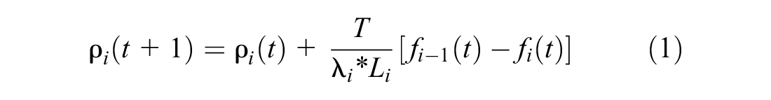
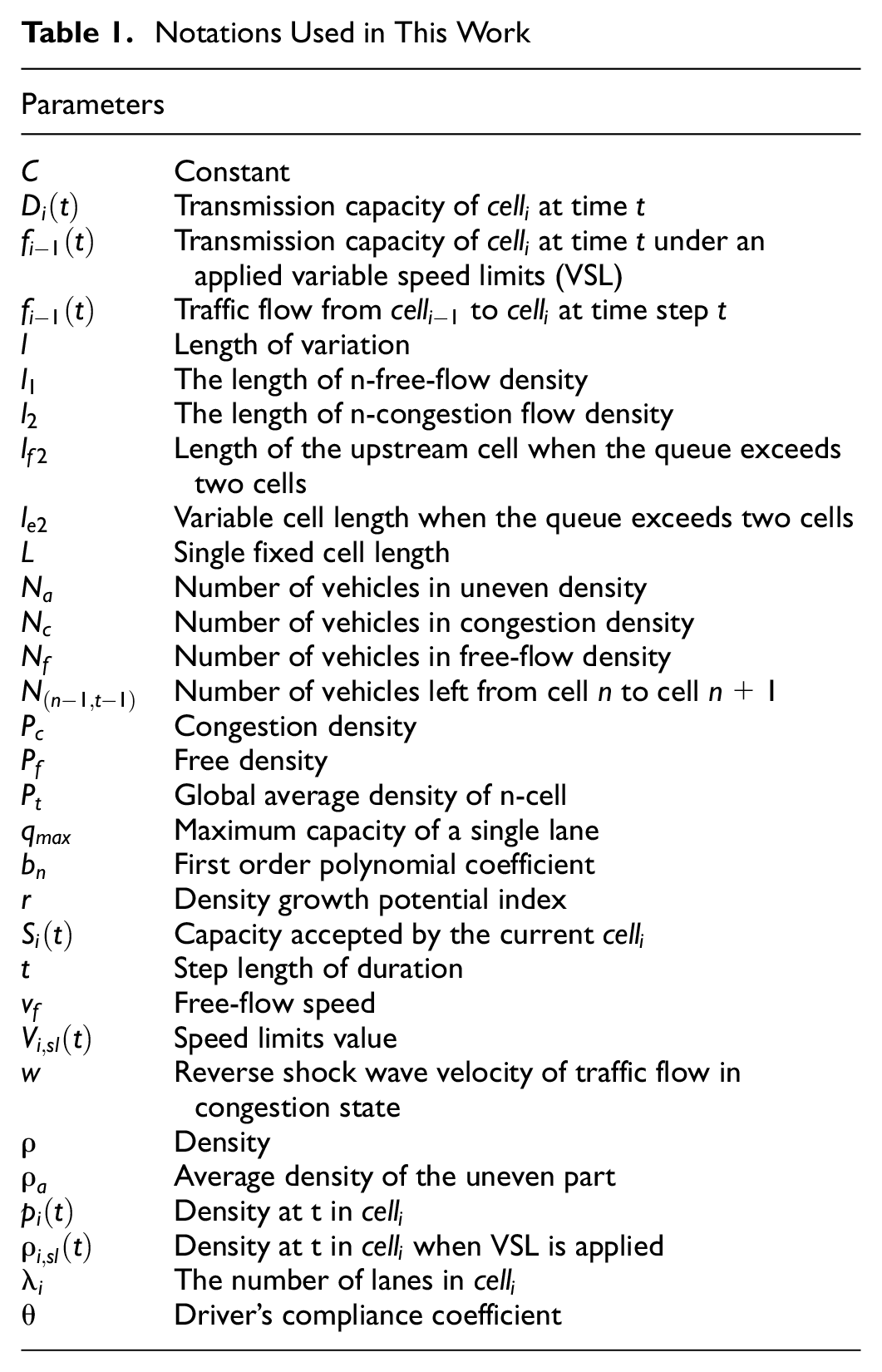
The CTM proposed by Daganzo ( 18 ) is a very popular macroscopic model in the field of modern transportation. This simple macroscopic traffic model based on vehicle dynamics has been proved to be consistent with fluid mechanics theory. The traditional model divides the highway into several cells of fixed length. Table 1 shows the notation used in this work. The renewal density equation of cell i is shown in Equation 1

ρ_{i} (t + 1) = ρ_{i} (t) + \frac{T}{λ_{i} * L_{i}} [f_{i - 1} (t) - f_{i} (t)]

(1)

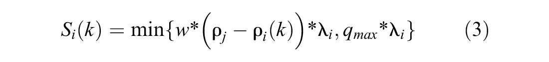
The supply and demand function of the cell is shown in Equations 2 and 3; the flow rate and critical density are given in Equations 4 and 5.

D_{i} (k) = \min {ρ_{i} (k) * v_{f} * λ_{i}, q_{\max} * λ_{i}}

(2)

S_{i} (k) = \min {w * (ρ_{j} - ρ_{i} (k)) * λ_{i}, q_{\max} * λ_{i}}

(3)

f_{i} (k) = \min {D_{i} (k), S_{i + 1} (k)}

(4)

ρ_{c =} \frac{q_{\max}}{v_{f}}

(5)

The combination of the CTM and VSL can relieve traffic pressure. Considering actual driving demands, the equation of the driver compliance index combined with VSL is shown in Equations 6 and 7.

Table 1.

Notations Used in This Work

Parameters
$C$	Constant
$D_{i} (t)$	Transmission capacity of $cel l_{i}$ at time $t$
$f_{i - 1} (t)$	Transmission capacity of $cel l_{i}$ at time $t$ under an applied variable speed limits (VSL)
$f_{i - 1} (t)$	Traffic flow from $cel l_{i - 1}$ to $cel l_{i}$ at time step $t$
$l$	Length of variation
$l_{1}$	The length of n-free-flow density
$l_{2}$	The length of n-congestion flow density
$l_{f 2}$	Length of the upstream cell when the queue exceeds two cells
$l_{e 2}$	Variable cell length when the queue exceeds two cells
$L$	Single fixed cell length
$N_{a}$	Number of vehicles in uneven density
$N_{c}$	Number of vehicles in congestion density
$N_{f}$	Number of vehicles in free-flow density
$N_{(n - 1, t - 1)}$	Number of vehicles left from cell $n$ to cell $n + 1$
$P_{c}$	Congestion density
$P_{f}$	Free density
$P_{t}$	Global average density of n-cell
$q_{\max}$	Maximum capacity of a single lane
$b_{n}$	First order polynomial coefficient
$r$	Density growth potential index
$S_{i} (t)$	Capacity accepted by the current $cel l_{i}$
$t$	Step length of duration
$v_{f}$	Free-flow speed
$V_{i, sl} (t)$	Speed limits value
$w$	Reverse shock wave velocity of traffic flow in congestion state
$ρ$	Density
$ρ_{a}$	Average density of the uneven part
$p_{i} (t)$	Density at t in $cel l_{i}$
$ρ_{i, sl} (t)$	Density at t in $cel l_{i}$ when VSL is applied
$λ_{i}$	The number of lanes in $cel l_{i}$
$θ$	Driver’s compliance coefficient

New demand and supply are given by Equations 8 and 9, while the speed limits are finally derived in Equation 10.

V_{i, sl} {(t)}^{'} = (1 + θ) * V_{i, sl} (t)

(6)

ρ_{i, sl} {(t)}^{'} = \frac{w * ρ_{j}}{w + V_{i, sl} {(t)}^{'}}

(7)

D_{i, sl} (t) = \min {ρ_{i} (t) * V_{i, sl} {(t)}^{'} * λ_{i}, q_{VSL} * λ_{i}}

(8)

S_{i, sl} (t) = \min {w * (ρ_{j} - ρ_{i} (t)) * λ_{i}, q_{VSL} * λ_{i}}

(9)

v_{i, sl} (t) = {\begin{matrix} \begin{matrix} \min {v_{f}, V_{i, sl} {(t)}^{'}} & ρ_{i} (t) \leq ρ_{i, sl} {(t)}^{'} \end{matrix} \\ \begin{matrix} w * (ρ_{j} - ρ_{i} (t)) / ρ_{i} (t) & ρ_{i} (t) > ρ_{i, sl} {(t)}^{'} \end{matrix} \end{matrix}

(10)

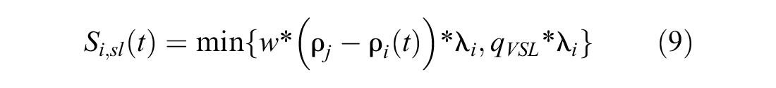
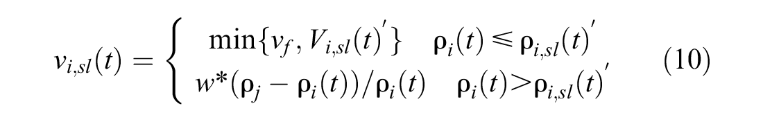
Figure 1 shows the basic triangle diagram of traffic flow, where the dotted line indicates the implementation of VSL. The VSL can improve the current upstream traffic conditions, but it will also reduce the speed and therefore the slope.

Figure 1.

Basic triangle diagram.

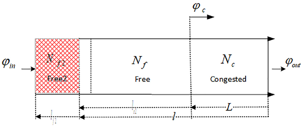
Figure 2 shows the control position of traditional VSL. When the road is congested, VSL can effectively relieve the pressure of the current road section, so VSL are applied to the CTM. The driver’s compliance coefficient is also taken into account.

Figure 2.

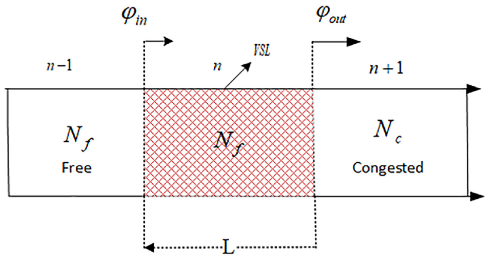
Traditional variable speed limits (VSL) control.

Modeling and Analysis of Crowded Front Section Position

The transition from free-flow density to congestion density is not instantaneous but gradual. So we analyze the transition from crowded cells to free cells. In Figure 3, the density distribution in the transition cell is not uniform. We first consider the variable-length CTM composed of two variable cells, one of which is the upstream free-flow cell $N_{f}$ , and the other is the downstream crowded cell $N_{c}$ , which acts as a buffer before the blocked cell area. The total length of a cell is L, of which the length of the free part is l, which changes with time, while the congested flow cell length is L- l. Free-flow cells are assumed to be in free density, while crowded cells are in crowded density. This means that the length of a crowded cell changes over time. Compared with the fixed cell, a variable-length cell only requires two state variables, and the key area is the junction of the two cells. It is worth noting that the length must be controlled flexibly. The cell density of free flow is denoted using $P_{f}$ , while that of crowded cells is $P_{c}$ , which can be written as shown in Equations 11 and 12.

N_{f} = l * P_{f}

(11)

N_{c} = (L - l) * P_{c}

(12)

In Figure 3, the density distribution of n is not uniform between the crowded cell and the free-flow cell. Therefore, we divide it into three states. The relationship between the density and the position of the three states is shown in Figure 4. The first part is the same as that with the previous free-flow density, and the second part is the transition from free-flow density to congestion density. The third part is in congestion density.

Figure 3.

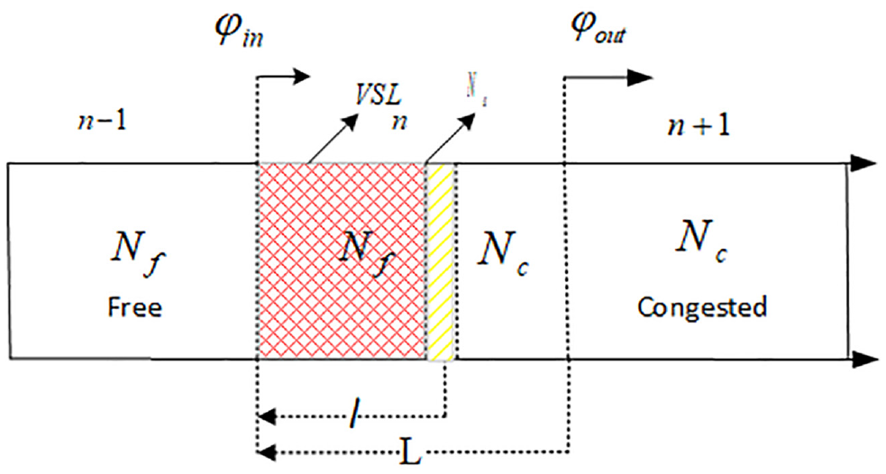
Variable-length cell process.

Figure 4.

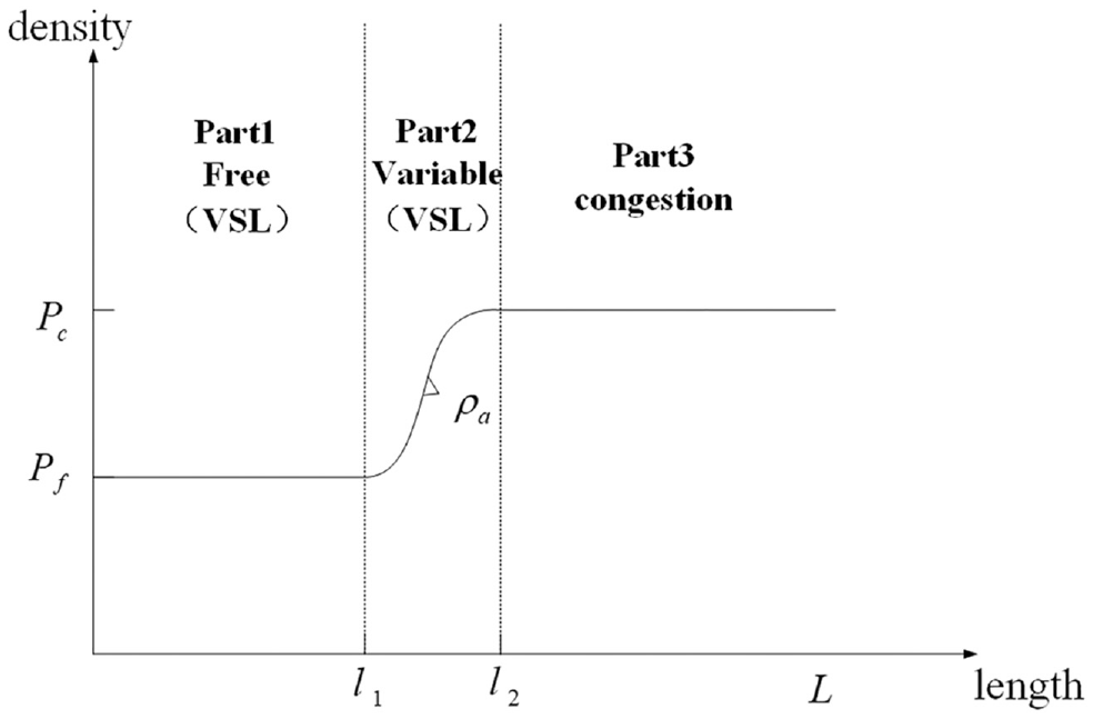
Relationship between the length and density of cell n.

In Part 2, firstly, when congestion first begins, the front-end vehicles start to queue slowly. Then, when more vehicles begin to flow in, the density increases rapidly. Finally, with increased congestion, its capacity decreases. As a result, the density increases slowly to the levels corresponding to congestion. The speed limits at the front section of congestion, start from $l_{1}$ and end at $l_{2}$ . It can, therefore, be seen as a logistic equation growth model, as given by Equation 13.

\frac{d ρ}{d l_{t}} = r ρ (\frac{P_{c} - ρ}{P_{c}})

(13)

where

$ρ$ is density,

$l$ is the length,

r is the density growth potential index, which depends on the traffic congestion, and

$P_{c}$ is the critical density.

We separate the variables on both sides to obtain by Equation 14 and integrate them as in Equation 15.

- \frac{r}{P_{c}} dl = \frac{1}{P_{c}} (\frac{1}{ρ - P_{c}} - \frac{1}{ρ}) dN

(14)

ρ = \frac{P_{c}}{1 + C e^{- rl}}

(15)

where C is a constant. From Figure 3, we can define the number of vehicles as a function of density which is shown Equations 16 to 18.

l_{1} * P_{f} = N_{f}

(16)

(l_{2} - l_{1}) * ρ_{a} = N_{a}

(17)

(L - l_{2}) * P_{c} = N_{c}

(18)

where $N_{C}$ is the number of vehicles left from cell n to cell $n + 1$ . The number of vehicles sent by the cell $n - 1$ to the cell n at time $t - 1$ ( $N_{(n - 1, t - 1)}$ ) can be written as in Equation 19. Because cell $n - 1$ is a free-flow cell, no vehicle will be left in it.

N_{f} + N_{a} = N_{(n - 1, t - 1)}

(19)

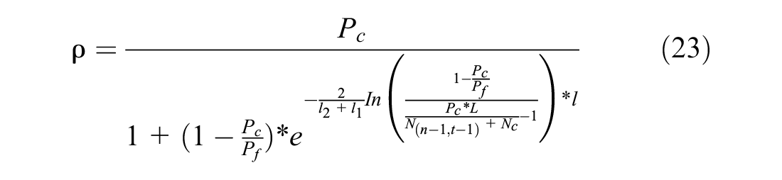
To better describe the current state of change and to simplify calculations, we define the density $P_{t}$ at the midpoint of part 2 as in Equation 20. The critical density $P_{c}$ and the initial quantity $P_{f}$ of the logistic equation can be obtained using this equation. C can be written as Equation 21. It can be concluded $r$ by Equation 22.

P_{t} = \frac{N_{(n - 1, t - 1)} + N_{c}}{L}

(20)

C = 1 - \frac{P_{c}}{P_{f}}

(21)

r = \frac{2}{l_{2} + l_{1}} In (\frac{1 - \frac{P_{c}}{P_{f}}}{\frac{P_{c} * L}{N_{(n - 1, t - 1)} + N_{c}} - 1})

(22)

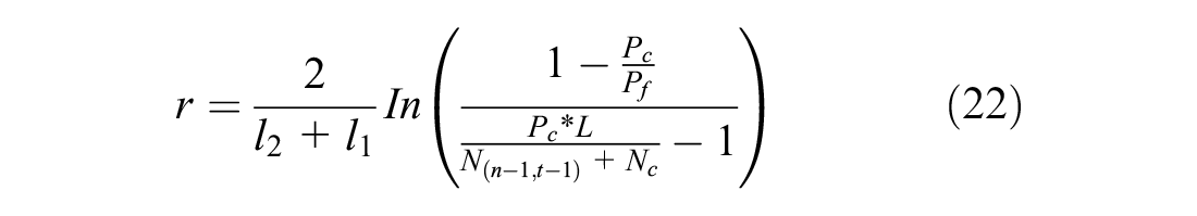
The final equation is shown in Equation 23.

ρ = \frac{P_{c}}{1 + (1 - \frac{P_{c}}{P_{f}}) * e^{- \frac{2}{l_{2} + l_{1}} In (\frac{1 - \frac{P_{c}}{P_{f}}}{\frac{P_{c} * L}{N_{(n - 1, t - 1)} + N_{c}} - 1}) * l}}

(23)

Because the middle part is in an uneven state and is more complicated, we define the average density of Part 2 using Equation 24 and the position of $l$ using Equation 25.

ρ_{a} = \frac{N_{(n - 1, t - 1)} - N_{c}}{L - \frac{N_{c}}{P_{c}} - 2 * l_{1}}

(24)

l = \frac{1}{\frac{2}{L - \frac{N_{c}}{P_{c}}} In (\frac{1 - \frac{P_{c}}{P_{f}}}{\frac{P_{c} L}{N_{(n - 1, t - 1)} + N_{c}} - 1})} * In (\frac{1 - \frac{P_{c}}{P_{f}}}{\frac{P_{c} * (L - \frac{N_{c}}{P_{c}} - l_{1})}{N_{(n - 1, t - 1)} - P_{f} * l_{1}} - 1})

(25)

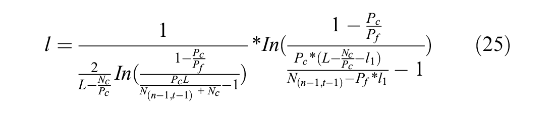
To better describe the current flow relationship and to simplify the formula, we apply a first order polynomial linear regression on the model and change Equations 23 to 26, which can be regarded as a univariate equation. We then write it in polynomial form as Equation 27.

\begin{matrix} In (\frac{P_{c} - ρ}{ρ}) & = In (1 - \frac{P_{c}}{P_{f}}) \\ - \frac{2}{l_{2} + l_{1}} In (\frac{1 - \frac{P_{c}}{P_{f}}}{\frac{P_{c} * L}{N_{(n - 1, t - 1)} + N_{c}} - 1}) * l \end{matrix}

(26)

ρ = \sum_{l_{1}}^{l_{2}} b_{n} l^{n}

(27)

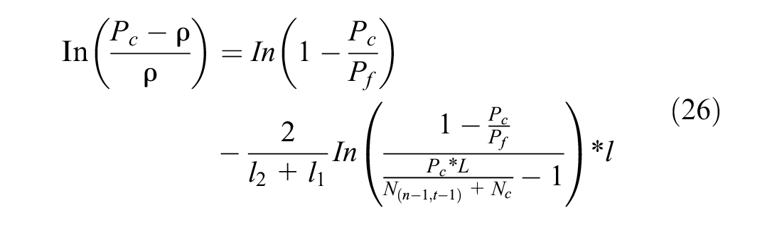
When Equation 27 is applied to the front end as a whole, it becomes a binary equation, which can then be optimized. When the traffic state is at its peak, the queue length increases greatly, and the process from the beginning of the congestion to its end will be faster.

The former and the latter nonlinear cases can be ignored. To simplify the equation, the higher-order term in Equation 27 can be ignored, and its influence on the equation is very small. And the middle linear growth can be retained, which can be regarded as the straight line given by Equation 28.

ρ = \frac{P_{c} - P_{f}}{L - \frac{N_{c}}{P_{c}} - 2 * l_{1}} * l + \frac{P_{c} - P_{f}}{L - \frac{N_{c}}{P_{c}} - 2 * l_{1}} * l_{1} - P_{f}

(28)

The results show that the length $l$ is as shown in Equation 29.

\begin{matrix} l = & \frac{(N_{(n - 1, t - 1)} - P_{f} * l_{1}) * (L - \frac{N_{c}}{P_{c}} - 2 l_{1})}{(L - \frac{N_{c}}{P_{c}} - l_{1}) * (P_{f} - P_{c})} \\ + \frac{P_{f} * ((L - \frac{N_{c}}{P_{c}} - 2 * l_{1})}{(P_{f} - P_{c})} - l_{1} \end{matrix}

(29)

Equation 28 gives the length of the congestion cell and can also be regarded as the current vehicle queue length. The setting position of the variable message sign can be selected according to the length of $l$ .

Remark 1: $N_{(n - 1, t - 1)}$ must be greater than $N_{f}$ , because the vehicles in $N_{f}$ belong to $N_{(n - 1, t - 1) .}$

Remark 2: The variable length needs to be bounded; it should not exceed the total length of the two fixed cells and should not be less than a certain length. The length limits depend on the actual situation. Note that the maximum value is allowed to exceed the length of two fixed cells or be less than 0. It is stipulated here that when the length change exceeds or is less than the limits, the variable cell of the current time period is set to be equal to the length of the fixed cell.

Numerical Analysis

The feasibility of the minimum interval of 2 min was verified using by numerical analysis. A minimum time interval of 1 s results in the consumption of more public resources. To solve the problem of resource allocation, the traffic flow state is described using a minimum time interval of 2 min. Taking 3,800 vehicles per hour (vph) as the constant flow input, a numerical simulation was carried out to analyze traffic flow within a period of 2 h and allow the analysis of congestion conditions. The following parameters and conditions were used: $q_{\max}$ = 1900 vph, $w$ = 18.1 km/h, $ρ_{c}$ = 19 veh/km, $ρ_{j}$ = 124 veh/km, $L_{i}$ = 0.83 km, $V_{f}$ = 100 km/h, $T =$ 30 $s$ , $θ = 0.1$ .

Figure 5 shows the time interval change diagram of 1 s, while Figure 6 shows the time interval change diagram of 2 min. Figure 5a shows the density and change position over the whole 2 h. It can be seen from Figure 6 that the overall change is the same, and there are some small gaps in the density of cell 6. For a more direct observation, Figures 5b and 6b show the changing state of the change part at 45 min. The overall change is almost the same. In only about 20 min, the 1 s case has a small advance position into cell 6 relative to 2 min, but the difference is not significant. We see that effect of the 2-min time interval is similar to that of a 1-s interval, but it is more convenient for practical implementations.

Figure 5.

Density and location changes (1 s): (a) changes within a 2-h period; and (b) changes in the middle 45 min.

Figure 6.

Density and location changes (2 min): (a) changes within a 2-h period; and (b) changes in the middle 45 min.

VSL Control Strategy With Dynamic Variable Message Signs

Selection of VSL Position

We first define the length of the cell changes and the length of the current blocking cell which is fixed and cannot be changed. We choose the second free-flow cell as the excess flow input.

As shown in Figure 7, the length changes of the two cells are similar. When the flow input is too high, the second free-flow cell length accepts the excess flow input and changes its length. This is expressed in Equation 30.

l_{e 2} = l - L

(30)

where $L$ is the fixed cell length, which is limited to three cells in this case.

Figure 7.

Three cell length changes.

The total length is the length of the three fixed cells, while the length variation range of the second free-flow cell is limited to the length of a fixed cell. Instead of a two-cell change, when three cells change, it goes back to the previous cell. While the changing length of the cell conflicts with the changing length of the two cells, the range of the changing length is different from that of the two cells. At the same time, a minimum range of variations must also be set. The advantage of the change here is that although the length change range is limited to the length of one cell, the indirectness expands the range of change. When the flow is not high, it changes within two cells. When the flow is high, the cell change length is extended to the second free-flow cell, which indirectly expands the range of change.

To provide a unified equation. We consider that, at this time, the cell length can be changed to any free-flow cell. For i, this is expressed in Equation 31.

l_{e_{(i + 1)}} = l - i * L

(31)

In Figure 8, the ordinary speed limits are positioned at the front end of the crowded cells to relieve the traffic pressure. However, the length change of the new variable cell is not only the free-flow cell in front of the current crowded cell, so a new speed limit change method is applied to the current cell. From Figure 5, the location of the new speed limit is related to the location of the changed cell. When the length of the cell changes to that of cell i, the speed limit position is ahead of the current change position. The congested area is relatively at the back end of the current change cell, while the speed limit area is in the front area.

Figure 8.

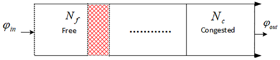
Dynamic cell length changes and speed limits selections.

While the length of the dynamic cell changes, the length of the upstream cell will also change as it shortens or increases. We thus define the length of its upstream cell as shown in Equation 32.

l_{f_{(i + 1)}} = 2 * L - l_{e_{(i + 1)}}

(32)

Because the length of the current dynamic cell is limited, it reverts to its previous value, which will affect the dynamic length change of the upstream cell.

When the crowded part of the cell changes, it is unreasonable to apply the VSL in the original location, so a new position must be selected in accordance with the length. Unlike the traditional VSL area selection, the vehicles in the congested area are actively moving forward, thereby changing the position of the congested area. The VSL is, therefore, reselected on this basis to distribute the vehicles in the congested area to more suitable areas.

When the speed limit area changes with the length and the length changes and leaves the current area, the speed slowly returns to the free-flow speed with a certain gradient.

Objective Function

The congestion of an expressway is reflected by the objective function, with the key aim being to reflect the overall performance of the current traffic conditions. Travel time has always been used as the objective function for determining the VSL control input, as shown in Equation 33.

J = T * \sum_{k = 1}^{N_{c} - 1} \sum_{i = 1}^{m} λ_{i} * L_{i} * ρ_{i} (k)

(33)

Because of the change in length, the new density equation is as follows:

ρ_{iv} (t + 1) = ρ_{i} (t) + \frac{T}{λ_{i} * L_{iv}} [f_{i - 1} (t) - f_{i} (t)]

(34)

where $ρ_{iv}$ represents the density of dynamic cell i at time t, and $L_{iv}$ represents the changed length of cell i at time t.

Then the new objective function is Equation 35:

J = T * \sum_{k = 1}^{N_{c} - 1} \sum_{i = 1}^{m} λ_{i} * L_{iv} * ρ_{iv} (k)

(35)

The time constraints for VSL are as shown in Equation 36:

| V_{i, sl} (K + 1) - V_{i, sl} (K) | \leq V_{gap}

(36)

Here, $V_{gap}$ represents the difference between the speed limit values over two consecutive moments. In this article, it is set to 10.

$V_{\min}$ and $V_{\max}$ are the maximum and maximum speed limits, set to 30 km/h and 100 km/h, respectively.

V_{i, sl} (K) \geq V_{\min}

(37)

V_{i, sl} (K) \leq V_{\max}

(38)

Experimental Simulation and Result Analysis

Simulation Environment

To ensure the accuracy of the experiment, a variable cell length experiment was carried out on an urban expressway about 10-km long. The CTM divided it into 12 cells, and we considered cells 8 and 9 as variable cells. The total length of the variable cells was equal to the total length of the two fixed cells. The fixed length of the constant cells was set to 0.83 km. We applied VSL in cell 8, and set the buffer cell and bottleneck cell to cells 9 and 10, respectively. The model was calibrated based on the actual urban expressway environment and traffic data were collected accordingly. The related parameters were obtained by cited references (31), and set as follows: $q_{\max}$ = 1900 vph, $w$ = 18.1 km/h, $ρ_{c}$ = 19 veh/km, $ρ_{j}$ = 124 veh/km, $L_{i}$ = 0.83 km, $V_{f}$ = 100 km/h, $T =$ 30 $s$ , $θ = 0.1$ .

In the following, Model A is the CTM with fixed VSL, Model B is the length-variable CTM under fixed VSL, and Model C is the length-variable CTM with selectable speed limits positions.

Simulation Result

Scenario 1

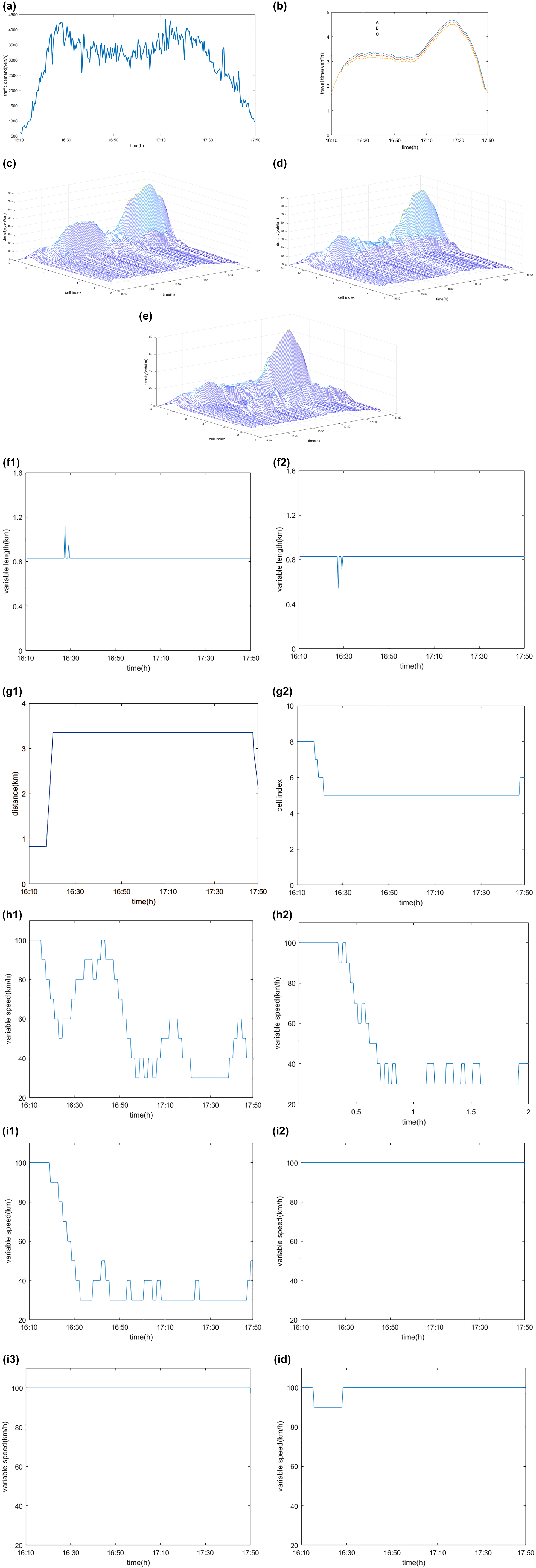
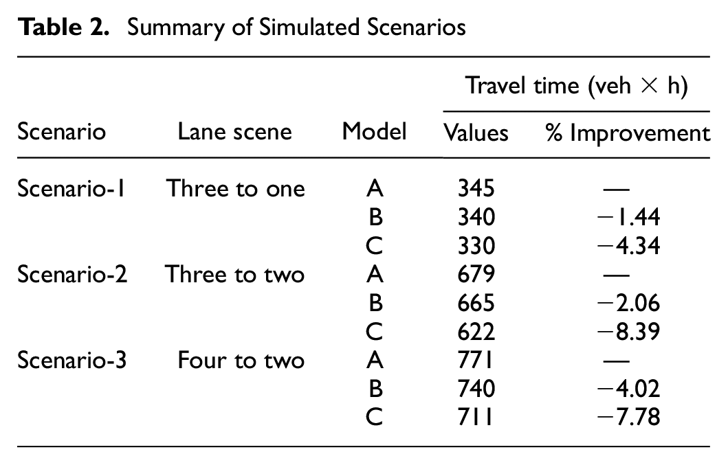
For Scenario 1 we considered a three-to-one lane closure as an example, from low density to high density. In Figure 9a, there are two peak periods and two non-peak periods in the traffic flow, and the volatility is relatively large. Figure 9b shows the comparison of the travel time obtained using the three models. It can be clearly seen that B and C start to work after congestion occurs. C performs better than B, especially when the traffic is more congested. B and C have decreased by 1.44% and 4.34% respectively. Figure 9, c to e , represent the densities of the three models.

Figure 9.

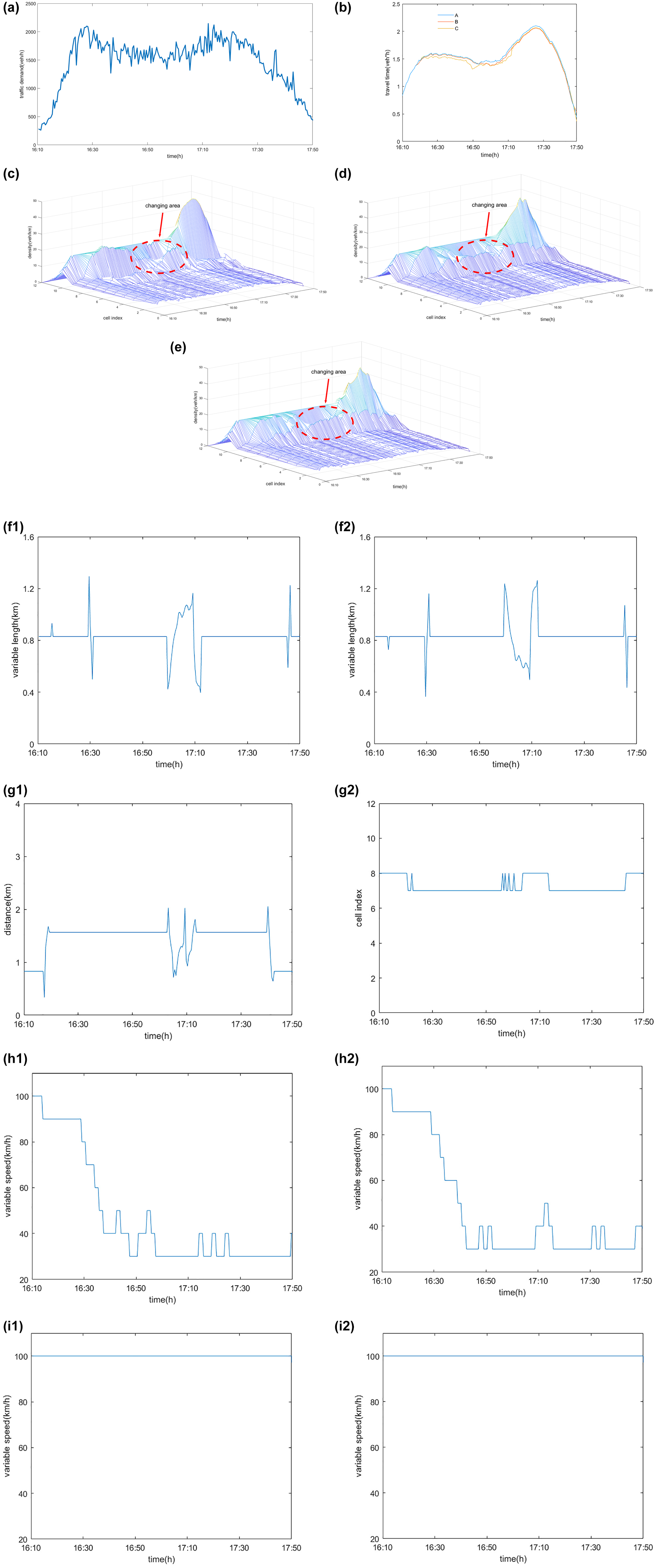
Three-to-one lane closure case: (a) traffic demand profile; (b) travel time profile; (c) density profile of Model A; (d) density profile of Model B; (e) density profile of Model C; (f) variable length (Model B): (I) cell 8 and (II) cell 9; (g) variable length and variable cell profile (Model C): (I) distance and (II) variable cell; (h) variable speed limit (VSL) trajectory profile 1: (I) model A and (II) model B; and (i) VSL trajectory profile 2 (Model C): (I) cell 5, (II) cell 6, (III) cell 7, and (IV) cell 8.

In Figure 9c, A has two high peaks at 16:30 and 17:30 during congestion, while Figure 9b shows a lower peak than the former because of the length change. In Figure 9e, given the change of the speed limit positions, the density value of C presents an increase in the vicinity of cell 7. The flow value in the middle section has decreased, thereby improving traffic efficiency.

Figure 9f’s I and II shows the length changes of cells 8 and 9 of B. When the traffic is light, the length begins to change. However, when the traffic flow increases, the length change loses its effect.

Figure 9g shows the position change of the variable cell C. Its length is the distance from cell 9. It can be seen from I and II that there are no changes in cells 5 and 6, while the lengths of cells 7 and 8 are changed more. As can be seen from II, the length change is a result of the increase in flow, so under the control of C, the length gradually changes from cell 8 to cell 7. And most of the time, the speed limits are at cell 7. Cell 8, as a variable cell in the middle, changes continuously.

Figure 9h shows the speed limits value of B and C, while Figure 9i shows the speed limits value of each cell of C. Under the control of C, the cell length changes only for cell 7, so the speed limits control only changes between cells 7 and 8.

Scenario-2

Scenario 2 shows the situation for a three-to-two closure. Figure 10a illustrates the traffic demand, simulating the peak period from 16:10 to 17:50, which is similar to Scenario 1. The travel time of B is slightly lower than that of A after 16:50 in Figure 10b, a 2.06% decrease, while C is significantly lower than the other two models, an improvement of 8.39% compared with A. As shown in Figure 10c, A has limited congestion-solving capacity, so in that case congestion extends rapidly, which causes an increase in density and further worsens the traffic situation. Figure 10d shows that B makes length changes to further improve the traffic conditions. B shows improved performance compared with A, while, as shown in Figure 10e, C effectively solves the congestion problem. There is a significant reduction of the peaks, but the improvement in the first peak is not obvious. However, after the first peak, the control begins to take effect when the speed-limiting cell moves to cell 6, which reduces the subsequent density. When it comes to the second peak, around 17:30, the density of C’s peak drops rapidly. Dynamic cell control can expand the length control range effectively, thereby using resources to the best advantage, easing traffic congestion, reducing bottlenecks, and improving traffic efficiency.

Figure 10.

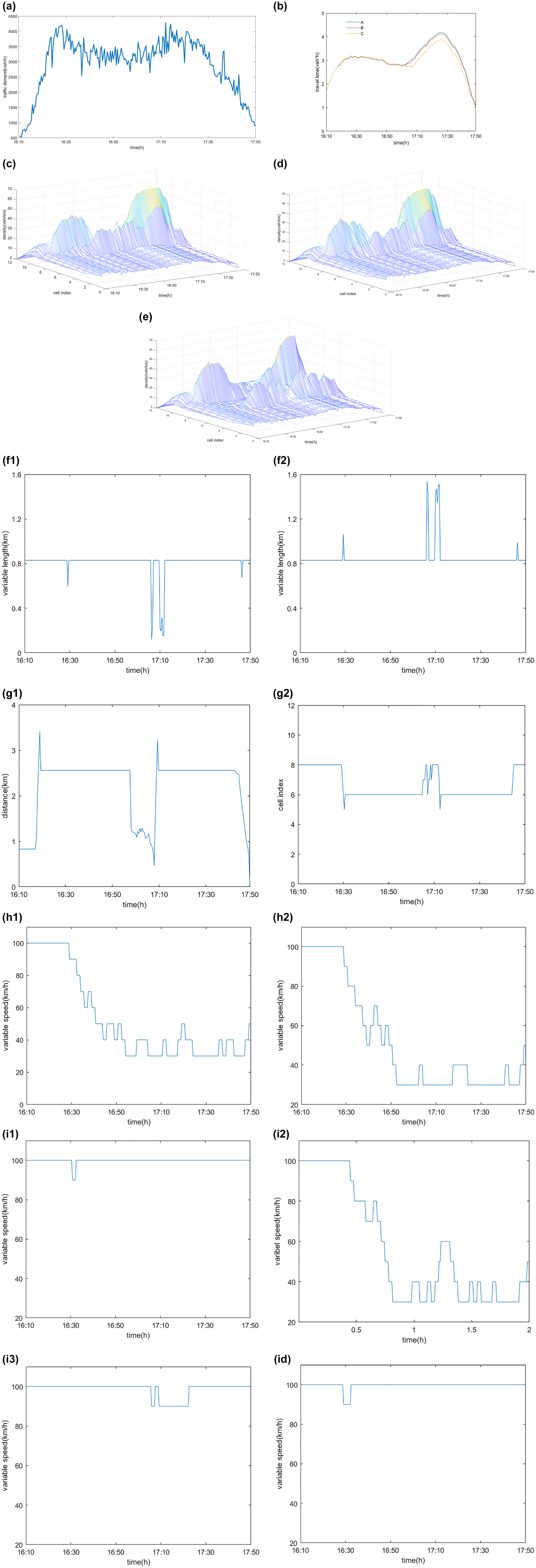
Three-to-two lane closure case: (a) traffic demand profile; (b) travel time profile; (c) density profile of Model A; (d) density profile of Model B; (e) density profile of Model C; (f) variable length (Model B): (I) cell 8 and (II) cell 9; (g) variable distance and variable cell profile (Model C): (I) distance and (II) variable cell; (h) variable speed limit (VSL) trajectory profile 1: (I) model A and (II) model B; and (i) VSL trajectory profile 2 (Model C): (I) cell 5, (II) cell 6, (III) cell 7, and (IV) cell 8.

Figure 10e shows the length change of B. In more crowded traffic conditions, the length does not change. The length control will be effective only when the traffic is relatively unblocked, thereby improving the traffic flow. Figure 10f shows that C achieves a significant improvement in length change compared with B. In model C, when there is no room for change in the current cell, the cell will extend to the subsequent cell. It can be clearly seen from II that as the flow increases, the changing cell also begins to move back, changing to cell 5, and staying in cell 6 for most of the time.

In Figure 10g, as length changes in cells 5 and 6, we can see the corresponding changes take place in the speed limit values in diagrams I to IV. However, when the current cell does not change, the speed will slowly return to its free-flow value. Figure 10h shows the speed values for A and B.

Scenario 3

Scenario 3 considers four-to-two lane closure as an example, and assumes similar traffic conditions, Figure 11, a and b , show the travel times obtained using the three models. It can be clearly seen that with the traffic increase, B and C improve the current traffic conditions and reduce travel times by 4.02% and 7.78%, respectively, compared with A. In Figure 11c, even with VSL, the current traffic conditions do not show great improvement because of the large traffic volume. In Figure 11d, B shows a decrease in the first peak because of the length change, but the crowded cell density has increased. In Figure 11e, the control of C is added, so the cell speed limits are always within the fifth cell, whose density decreases correspondingly, while the peak remains relatively low.

Figure 11.

Four-to-two lane closure case: (a) traffic demand profile; (b) travel time profile; (c) density profile of Model A; (d) density profile of Model B; (e) density profile of Model C; (f) variable length (Model B): (I) cell 8 and (II) cell 9; (g) variable distance and variable cell profile (Model C): (I) distance and (II) variable cell; (h) variable speed limit (VSL) trajectory profile 1: (I) model A and (II) model B; and (i) VSL trajectory profile 2 (Model C): (I) cell 5, (II) cell 6, (III) cell 7, and (IV) cell 8.

In Figure 11f, B does not change its length anymore because of the large flow at the back end. In Figure 11g, the length extends from cell 7 to 6 in II, and finally remains at cell 5, thus indirectly expanding the length. As shown in Figure 11h, I is the speed of A while II is the speed of B. In Figure 11i, in IV, the speed limits stay in cell 8 over a period of time, and then move backward sequentially. In II, the speed limits stay in cell 5, and finally return to cell 8. When traffic is more congested, C also shows an improvement as it causes a change in the cell lengths, thereby improving traffic conditions.

Conclusion

In this paper, a new length variation model is proposed, which can describe the non-uniform traffic flow parts better compared with existing fixed element models. At the same time, a new speed limit location selection scheme is presented. The speed limit location is selected according to the change of cell length. This method is superior to the traditional models in dealing with traffic problems, and can adapt to different traffic conditions. It can alleviate traffic congestion and improve traffic efficiency, especially in cases of traffic emergencies and other sudden increases or decreases in traffic flow.

The feasibility of the new strategy is verified through numerical analysis. In practice, to reduce the computational load and optimize calculations, the control under a certain time interval is similar to the theory. The effectiveness of the strategy is verified through simulations, through a comparison of different strategies applied to several models. We compared performance of different models from low flow to high flow under the same conditions. Table 2 shows the results of each part of the experiment. The results clearly show that the new control mode is superior to other options. The highway driving time is shortened and the traffic congestion is alleviated. Compared with other strategies, the new strategy has a certain effect under different traffic conditions. It provides a new decision-making reference for better adaptation to traffic conditions for future intelligent and driverless.

Table 2.

Summary of Simulated Scenarios

Scenario	Lane scene	Model	Travel time (veh × h)
Scenario	Lane scene	Model	Values	% Improvement
Scenario-1	Three to one	A	345	—
		B	340	−1.44
		C	330	−4.34
Scenario-2	Three to two	A	679	—
		B	665	−2.06
		C	622	−8.39
Scenario-3	Four to two	A	771	—
		B	740	−4.02
		C	711	−7.78

Although the total travel time is optimized in this paper, the consideration of vehicle exhaust emissions is insufficient. In practice, all vehicles need to be networked to ensure the accuracy and real-time acquisition of data. In the future research, we will, therefore, also consider exhaust emission and information acquisition, as well as transportation, network, and environmental benefits.

The authors confirm contribution to the paper as follows: study conception and design: X. Jiajie Hou; data collection: Y. Minghui Ma; analysis and interpretation of results: X. Jiajie Hou; draft manuscript preparation: Y. Minghui Ma. Z. Jiacheng Xiao. All authors reviewed the results and approved the final version of the manuscript.

Footnotes

Declaration of Conflicting Interests

The author(s) declared no potential conflicts of interest with respect to the research, authorship, and/or publication of this article.

Funding

The author(s) disclosed receipt of the following financial support for the research, authorship, and/or publication of this article: This work was partially supported by Natural Science Foundation of Shanghai (No.20ZR1422300), Program for Professor of Special Appointment (Eastern Scholar) at Shanghai Institutions of Higher Learning, Program of Shanghai Academic/Technology Research Leader (No.21XD1401100), and Technical Service Platform for Vibration and Noise Testing and Control of New Energy Vehicles (No.18DZ2295900).

ORCID iDs

Jiajie Hou

Minghui Ma

Jiacheng Xiao

References

Zhang

Ioannou

P. A.

Combined Variable Speed Limits and Lane Change Control for Highway Traffic. IEEE Transactions on Intelligent Transportation Systems, Vol. 18, No. 7, 2017, pp. 1812–1823.

Zhang

Liang

Dynamic Control Cycle Speed Limits Strategy for Balanced Reduction of Travel Time and Emissions. Modern Physics Letters B, Vol. 35, No. 9, 2021, p. 2150153.

Allaby

Hellinga

Bullock

Variable Speed Limits: Safety and Operational Impacts of a Candidate Control Strategy for Freeway Applications. IEEE Transactions on Intelligent Transportation Systems, Vol. 8, No. 4, 2007, pp. 671–680.

Liu

Ghosal

Chuah

C.-N.

Zhang

H. M.

Reducing Greenhouse Effects via Fuel Consumption-Aware Variable Speed limits (FC-VSL). IEEE Transactions on Vehicular Technology, Vol. 61, No. 1, 2012, pp. 111–122.

Raadsen

M. P. H.

Bliemer

M. C. J.

Variable Speed Limits in the Link Transmission Model Using an Information Propagation Method. Transportation Research Part C: Emerging Technologies, Vol. 129, 2021, pp. 1031–1084.

Smulders

Control of Freeway Traffic Flow by Variable Speed Signs. Transportation Research Part B: Methodological, Vol. 24, No. 2, 1990, pp. 111–132.

Papageorgiou

Kosmatopoulos

Papamichail

Effects of Variable Speed Limits on Motorway Traffic Flow. Transportation Research Record: Journal of the Transportation Research Board, 2008. 2047: 37–48.

Duret

Ahn

Buisson

Lane Flow Distribution on a Three-Lane Freeway: General Features and the Effects of Traffic Controls. Transportation Research Part C: Emerging Technologies, Vol. 24, 2012, pp. 157–167.

Knoop

V. L.

Duret

Buisson

Van Arem

Lane Distribution of Traffic Near Merging Zones Influence of Variable Speed Limits. Proc., 13th International IEEE Conference on Intelligent Transportation Systems, Funchal, Portugal, IEEE, New York, 2010, pp. 449–480.

10.

Deo

De Schutter

Hegyi

Model Predictive Control for Multi-Class Traffic Flows. IFAC Proceedings Volumes, Vol. 42, No. 15, 2009, pp. 25–30.

11.

Kim

Cassidy

M. J.

A Capacity-Increasing Mechanism in Freeway Traffic. Transportation Research Part B: Methodological, Vol. 46, No. 9, 2012, pp. 1260–1272.

12.

Carlson

R. C.

Papamichail

Papageorgiou

Messmer

. Optimal Motorway Traffic Flow Control Involving Variable Speed Limits and Ramp Metering. Transportation Science, Vol. 44, No. 2, 2010, pp. 238–253.

13.

Carlson

R. C.

Papamichail

Papageorgiou

Local Feedback-Based Mainstream Traffic Flow Control on Motorways Using Variable Speed Limits. IEEE Transactions on Intelligent Transportation Systems, Vol. 12, No. 4, 2011, pp. 1261–1276.

14.

Hegyi

Hoogendoorn

S. P.

Schreuder

Stoelhorst

Viti

SPECIALIST: A Dynamic Speed Limits Control Algorithm Based on Shock Wave Theory. Proc., IEEE Conference on Intelligent Transportation Systems, Beijing, China, IEEE, New York, 2008, pp. 827–832.

15.

Chen

Ahn

Variable Speed Limits Control for Severe Non-Recurrent Freeway Bottlenecks. Transportation Research Part C: Emerging Technologies, Vol. 51, 2015, pp. 210–230.

16.

Walraven

Spaan

M. T. J.

Bakker

Traffic Flow Optimization: A Reinforcement Learning Approach. Engineering Applications of Artificial Intelligence, Vol. 52, 2016, pp. 203–212.

17.

Cao

Variable Speed Limits Strategies’ Analysis With Cell Transmission Model on Freeway. Modern Physics Letters B, Vol. 31, No. 24, 2017, p. 1750219.

18.

Daganzo

C. F.

The Cell Transmission Model: A Dynamic Representation of Highway Traffic Consistent With the Hydrodynamic Theory. Transportation Research Part B: Methodological, Vol. 28, No. 4, 1994, pp. 269–287.

19.

Ziliaskopoulos

A. K.

Lee

A Cell Transmission Based Assignment-Simulation Model for Integrated Freeway/Surface Street Systems. Transportation Research Record: Journal of the Transportation Research Board, 1996. 1701: 12–23.

20.

Erera

A. L.

Lawson

T. W.

Daganzo

C. F.

Simple, Generalized Method for Analysis of Traffic Queue Upstream of a Bottleneck. Transportation Research Record: Journal of the Transportation Research Board, 1998. 1646: 132–140.

21.

Zhao

X.-M.

Xie

D.-F.

Wang

W.-W.

Geng

Calibrating and Modeling Expressway With Different Ramp Distances on Beijing 3rd Ring Road. Procedia - Social and Behavioral Sciences, Vol. 138, 2014, pp. 37–44.

22.

Kim

Choi

Yeo

Extended Urban Cell Transmission Model Using Agent-Based Modeling. Procedia Computer Science, Vol. 170, 2020, pp. 354–361.

23.

Asano

Sumalee

Kuwahara

Tanaka

Dynamic Cell Transmission-Based Pedestrian Model With Multidirectional Flows and Strategic Route Choices. Transportation Research Record: Journal of the Transportation Research Board, 2007. 2039: 42–49.

24.

Szeto

W. Y.

Ghosh

Basu

O’Mahony

Multivariate Traffic Forecasting Technique Using Cell Transmission Model and SARIMA Model. Journal of Transportation Engineering, Vol. 135, No. 9, 2009, pp. 658–667.

25.

Kong

Q. J.

Shu

Liu

(eds.). Urban Traffic Flow Prediction Based on Road Network Model. Proc., 9th IEEE International Conference on Networking, Sensing and Control, Beijing, China, IEEE, New York, 2012, pp. 334–339.

26.

Chen

Liu

Qiu

Liu

Sangaiah

A. K.

Latency Estimation Based on Traffic Density for Video Streaming in the Internet of Vehicles. Computer Communications, Vol. 111, 2017, pp. 176–186.

27.

Chen

Tian

Fortino

Zhang

Humar

Cognitive Internet of Vehicles. Computer Communications, Vol. 120, 2018, pp. 58–70.

28.

Roopa

M. S.

Siddiq

S. A.

Buyya

Venugopal

K. R.

Iyengar

S. S.

Patnaik

L. M.

DTCMS: Dynamic Traffic Congestion Management in Social Internet of Vehicles (SIoV). Internet of Things, Vol. 16, 2020, pp. 1003–1011.

29.

Zhang

Liu

Huang

Chen

Hao

Cunningham

Early

An Optimal Control Strategy Design for Plug-In Hybrid Electric Vehicles Based on Internet of Vehicles. Energy, Vol. 228, No. 3, 2021, p. 120631.

30.

Zhang

Liang

Dynamic Control Cycle Speed Limit Strategy for Improving Traffic Operation at Freeway Bottlenecks. KSCE Journal of Civil Engineering, Vol. 25, No. 2, 2020, pp. 692–704.

31.

Liu

-B.,P.

Wang

C.-C.

Development of control strategy of variable speed limits for improving traffic operations at freeway bottlenecks. Journal of Central South University, Vol. 21, No. 6, 2014, pp. 2526–2538.