Life Cycle Cost Analysis of High Friction Surface Treatment Applications

Abstract

Life cycle cost analyses for high friction surface treatment (HFST) applications were executed relying on a Microsoft Excel program developed by the researchers. Calcined bauxite (CB), five CB alternatives, and epoxy binder were utilized in the HFST applications. The aggregates’ performances were evaluated through the aggregate image measurement system (AIMS) before and after Micro-Deval polishing. The performance of the HFST applications was evaluated by the dynamic friction tester (DFT) and British pendulum (BP). The major purpose of this program was to present a rational method for converting different input data (project and material specifics) to comparable output data (net present value [NPV]) that facilitated comparison between different alternatives. The project specifics included traffic data, highway classification, and geometric design data. The material specifics data were AIMS results, DFT results, BP results, and materials and shipping costs. Three prediction models were selected to relate the performance test results to skid number (SN). The rehabilitation matrix, proposed by the researchers, was used to make the decision to maintain the HFST. This was conducted by comparing the predicted terminal SN and the recommended terminal SN (controlled by the user). The program output showed that Meramec River Aggregate and Flint HFST applications had the lowest NPVs, followed by Steel Slag HFST application, and then Earthworks HFST application. Nevertheless, Rhyolite HFST application showed the highest NPVs followed by the CB HFST application. The cost of the resin was dominant over the total cost of the HFST application.

Keywords

infrastructure infrastructure management and system preservation pavement management systems life cycle cost analysis (LCCA)materials aggregates aggregate sources aggregate tests asphalt mixture evaluation and performance skid and friction resistance

Maintaining an appropriate amount of pavement friction is critical for safe driving and crash reduction. Surface treatments are primarily used to extend the pavement life and improve skid resistance ( 1 ). Among surface treatment applications, high friction surface treatment (HFST) provides better skid resistance. HFST is used to reduce roadway crashes on horizontal curves or other risky locations (e.g., high-speed declaration ramps, steep grades, intersections with high-speed approaches, transition lanes, and pedestrian crossings) (1 –5). HFST is determined to be a cost-effective safety treatment consisting of a polymer resin layer, that is used to bond the pavement with 3–4 mm maximum size high friction aggregates. These aggregates have high angularity, high texture, and high polishing resistance (e.g., calcined bauxite [CB], flint/chert, slags, or granite) (1, 2, 5 –8). Resin binder, such as epoxy resin, polyester resin, polyurethane resin, acrylic resin, or methyl methacrylate, is spread over the pavement surface to bond this surface with the aggregate layer (2, 5, 6). The most common resin binder in HFST is epoxy resin, a two-part binder that consists of a resin (extender) and an epoxy (hardener) ( 5 ).

Performance is the primary goal in considering the friction of HFST application, which is identified through the microtextures of aggregates and the macrotextures of the surfaces (2, 9). The macrotexture depends on the aggregate gradation, compaction level, and mixture design. The aggregate microtexture is affected by the shape and texture of the aggregates (9 –12). The service life of HFST varies based on climate and roadway characteristics such as traffic volume, mix types, nature of traffic movement, and roadway geometry. For correctly applied HFST, the service life of HFST ranges from 7 to 12 years. Vendors reported 5 years of service life for HFST applied on roadways with traffic volumes of approximately 50,000 vehicles per day (vpd) and 5 to 8 years for traffic volumes of around 15,000 vpd ( 1 ). The HFST cost—the materials, labor, equipment, and traffic control—ranges from $21/yd² to $26/yd² as of 2017, which decreases in larger projects. It was reported that the cost of the epoxy resin, equipment, and labor were significant drivers of the project bid, not the cost of the aggregate ( 1 ).

The purpose of using life cycle cost analysis (LCCA) is to evaluate the short-term and long-term economic efficiencies between competing alternatives ( 13 ) (i.e., HFST applications using CB and alternative aggregates). The LCCA incorporates initial and discounted future costs incurred by the agency, user, and other stakeholders over the lifetime of the proposed alternatives (14, 15). The initial cost includes—but is not limited to—mobilization, labor, epoxy binder, correct gradation effort costs, and the aggregate itself.

The main objective of this study was to develop a life cycle cost (LCC) program using Microsoft Excel to present a rational method for converting different input data (material and project specifics) into comparable output data (net present value [NPV]). This LCC program facilitated comparison among different alternatives. The program was based on using aggregate image measurement system (AIMS), dynamic friction tester (DFT), or British pendulum (BP) results. The LCC program’s user can select one of the AIMS, DFT, or BP to perform the LCCA based on the available input data. Finally, a comparative LCCA study was conducted to identify the best HFST application.

Materials

CB and five alternatives were selected for testing; these aggregates were crushed stone. The alternative aggregates were Meramec River Aggregate, Flint, Earthworks, Rhyolite, and Steel Slag. These aggregates were selected as possible alternatives to CB. Moreover, these alternative aggregates are available in the U.S.A., note Table 1. Aggregate sources were discussed based on a review with the engineers of the MoDOT ( 16 ). Steel Slag was selected based on previous findings by other researchers who recommended its use in HFST application as an alternative to CB ( 17 ). In addition, a two-component (A and B) epoxy binder with a 1:1 mixing ratio by volume or a 1.18:1.00 mixing ratio by weight was utilized in the preparation of the coupons for the BP test and the HFST applications on the hot mix asphalt (HMA) slabs used for the DFT. Aggregates and epoxy binder information is presented in Table 1. The aggregate gradation for the received aggregates, as-delivered gradation, is presented in Table 2. Figure 1 shows the particles’ shapes of CB and alternatives.

Table 1.

Aggregates and Used Epoxy Binder Information ( 16 )

Aggregate name	Commercial names and received sizes	Details/Sources
Calcined bauxite (CB)	Calcined bauxite GRIP grain: MAS (#4)	Bauxite is mined because it is almost found near the surface of the terrain. Calcined bauxite is produced by sintering high-alumina Bauxite at high temperatures/Great Lakes Minerals, LLC in Wurtland, Kentucky, U.S.A. The GRIP grain CB is specifically produced for HFST. The typical aluminum oxide content for the CB was 87.5%, which was just above the 87% minimum found in most of the HFST specifications. The GRIP grain bauxite product had a certificate of analysis that guaranteed that the material provided to us had an 88.65% aluminum oxide content. This was inside the range for the AASHTO MP 41-19 (85%–89%).
Earthwork solution: Natural calcined bauxite	Earthworks #6 × #16: MAS (#6)	The Earthwork solution is known as natural calcined bauxite. It was named Earthworks in this study to avoid any confusion between it and the control CB. The rock formation is layered. It is blasted and then mined and crushed at quarry/Earth Work Solutions in Gillette, Wyoming, U.S.A.
Meramec river aggregate: Coarse manufactured sand	Meramec river aggregate: MAS (3/8′′)	The material is a deposit of sand and gravel that has been in the Meramec basin for thousands of years. The layers of material are overburden (topsoil) then the gravel, then sometimes a thin layer of sticky mud, then the sand on the bottom/Winter Brothers Material Company in Saint Louis, Missouri, U.S.A. This aggregate is used in road construction as well as concrete aggregate.
Steel slag	Steel Slag 1′′ × 0: MAS (1′′)	Steel Slag is a by-product of steel making/Harsco Inc in Muscatine, Iowa, U.S.A. The Steel Slag is typically used in surface courses to enhance the strength, durability, and frictional characteristics of the road.
Rhyolite: Iron Mountain trap rock	Rhyolite 1/2′′ × 0: MAS (1/2′′), and Rhyolite #6 × #16: MAS (#6).	The rock formation is igneous. Volcanic, Lead Belt area of Missouri, Ironton. Being volcanic in nature it was formed during heavy volcanic activity in Missouri, the Lead Belt area is known for Iron Ore, Lead smelting and production, granite and trap rock/Fred Weber in Maryland Heights Missouri, U.S.A. This aggregate is typically used for road and railroad construction as well as a chip seal.
Flint/chat/chert	Flint #6 × #16: NMAS (#6).	Flint is a sedimentary rock composed of microscopic crystals of quartz (silica, SiO₂). It is commonly found in the dumps at the abandoned lead and zinc mines/Williams Diversified Materials in Baxter Springs, Kansas, U.S.A. This aggregate is specifically produced for friction-enhancing surface treatments.
Epoxy binder name	Epoxy binder type	Notes
FasTrac CE330 Epoxy Binder. Low Modulus Epoxy Polymer Binder	Two-component epoxy binder	The epoxy binder had a bond strength of 2 ksi after 2 days & 2.8 ksi after 14 days and a tensile elongation of 40%

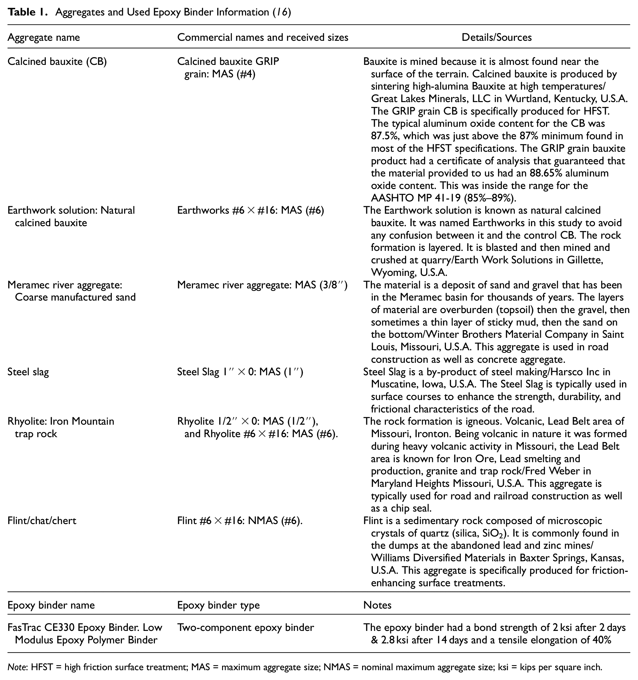
Note: HFST = high friction surface treatment; MAS = maximum aggregate size; NMAS = nominal maximum aggregate size; ksi = kips per square inch.

Table 2.

Gradations of the Aggregates

Aggregate type (Size)	Retained percentage (%)
Aggregate type (Size)	1/2′′	3/8′′	#4	#8	#16	#30	#50	#100	#200	Pan
Calcined Bauxite (GRIP Grain with MAS #4)	0	0	0	50	48	2	0	0	0	0
Earthworks (#6 × #16)	0	0	0	38	60	2	0	0	0	0
Meramec river aggregate (coarse manufactured sand with MAS 3/8′′)	0	0	0	23	34	23	12	6	2	0
Steel slag (1′′ × 0)	0	57	30	8	2	1	0	0	1	1
Rhyolite (1/2′′ × 0)	2	15	36	21	11	6	3	2	2	2
Rhyolite (#6 × #16)	0	0	1	56	39	3	1	0	0	0
Flint (#6 × #16)	0	0	0	53	46	1	0	0	0	0

Note: MAS = maximum aggregate size.

Figure 1.

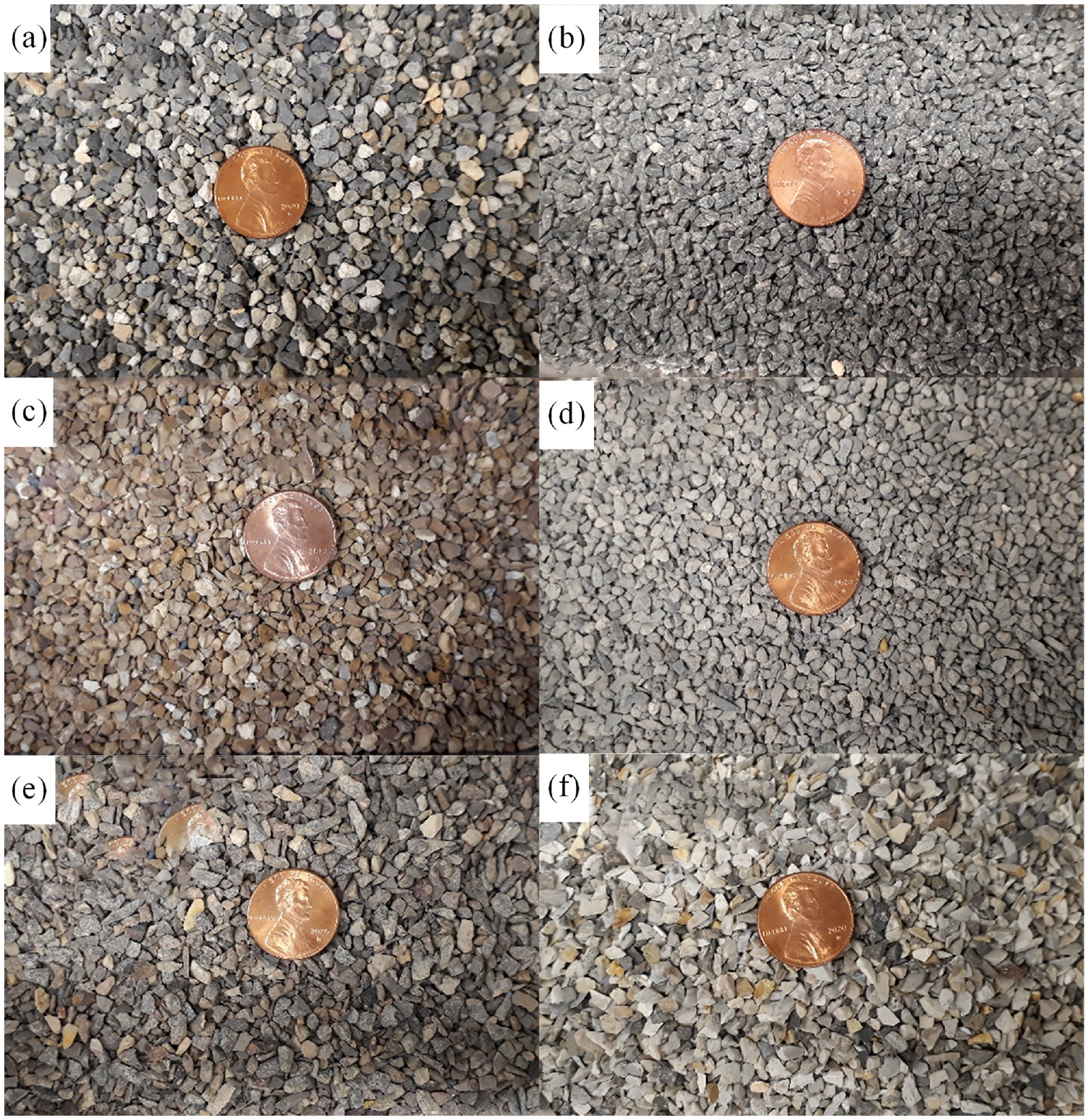
Particles’ shapes of calcined bauxite and alternatives with #6 × #16 gradation: (a) Calcined bauxite, (b) Earthworks, (c) Meramec river aggregate, (d) Steel slag, (e) Rhyolite, and (f) Flint.

Methods

Four tests were utilized in this study: one durability test and three performance tests. The durability test was the Micro-Deval (MD). The performance tests were the AIMS test, BP test, and dynamic friction test.

Micro-Deval

The aggregates were tested for their degradation/polish resistances in the MD apparatus. The MD test was utilized to explore aggregates’ durabilities and resistances to polishing and grinding in the water (5, 9, 18). The coarse aggregate MD test was run following ASTM D6928 – 17 on aggregate size (passing from sieve 3/8′′ and retained on #4 [3/8′′–#4]). The test was run for 105 min and 180 min. Each aggregate had one sample tested for each run time.

Aggregate Image Measurement System

After the samples were tested using the MD test at 105-min and 180-min polishing times, samples of all the aggregates were tested in the AIMS2 along with aggregate samples before MD polishing. AIMS analyses were conducted to explore changes in texture and angularity indices after MD polishing. The angularity indices were identified by the irregularity of particle surfaces using black and white images; the surface texture indices were determined using the wavelet analysis method ( 9 ). The AIMS device consists of a computer-automated unit that includes a circular measuring tray. The system is equipped with top lighting, backlighting, and a high-resolution digital camera. This camera, built into AIMS2, delivered improved gray texture images by providing precise control of image intensity. The AIMS Software^© consists of a series of algorithms that objectively determine the properties of aggregate shape on a macro-scale, features >0.5 mm in size, (e.g., angularity). Moreover, the system detects features on the micro-scale, features <0.5 mm in size, (e.g., surface texture).

The aggregates were placed in the trough of the circular tray, and the tray was rotated to move the aggregates under the camera unit. When the tray moved, the aggregates moved under the camera and several images were taken for measuring angularity. The positions of aggregates were recorded so that the camera could return to the centroid of the particles for texture image acquisition. The results of the AIMS software for each individual particle were included along with baseline statistical values of the scanned sample (e.g., mean, standard deviation, and cumulative distribution of measurements for each aggregate shape property).

Dynamic Friction Test

Loose asphalt mixtures were acquired from an asphalt plant in Pullman, WA, U.S.A. They were dense-graded hot asphalt mixtures with a 12.5-mm nominal maximum aggregate size. These mixtures were the standard HMA used and approved by the University of Idaho ( 19 ). The plant mixtures were reheated, and the HMA slabs (20 in. × 20 in. × 2 in.) were prepared and compacted in the laboratory using a small plate compactor. Epoxy binder was applied to the surface of the HMA slabs before the aggregates with a size (#6–#8) were spread.

A three-wheel polishing device (TWPD) was used to polish the HFST applications on the HMA slabs. The researchers measured the coefficient of friction (COF) at different polishing cycle numbers (i.e., 0 cycles [initial], 70k cycles, and 140k cycles [terminal]). The COF was measured using a DFT at 40 km/h (DFT₄₀) following ASTM E1911 – 19. The friction was measured in wet conditions. The results were based on the average of two replicates (two test slabs).

British Pendulum Test

The aggregate coupons were prepared using CB, five CB alternatives, plaster, and epoxy binder. A ready-mix plaster with a weight of 12 g was added and spread on the bottom of the metal molds, and the aggregates were embedded into the plaster so that the plaster prevented the epoxy binder from flowing into the gaps between the aggregates’ particles. The aggregates sizes were #6–#8 and #4–#6. Additional plaster was painted onto the sides of the molds using a small brush to completely cover the surface and keep the epoxy from adhering to the metal molds. The prepared epoxy binder was poured on the aggregates to fill the remaining part in the metal mold. The aggregate coupons were left in the metal molds at room temperature for 4–6 h. Finally, the aggregate coupons were removed from the metal molds and washed with water to remove the plaster layer.

The prepared coupons were tested for their initial British pendulum number (BPN)—the values were recorded as BPN before polishing—and each coupon was tested five times. The BP test was run following AASHTO T 278-90 (2017). The test aimed to measure the surfaces’ frictional properties using the BP. A slider with 1/4-in. × 1-in. × 1 1/4-in. dimensions was used.

The aggregates coupons were polished following AASHTO T 279-18 with the British wheel. The test simulated the polishing action that occurs to aggregates in the field. For each run, 14 aggregate coupons were clamped around the periphery of the road wheel. The speed of the road wheel was set to 320 ± 5 rpm. The pneumatic-tired wheel was lowered to bear on the surface of the aggregate coupons with a total load of 391.44 ± 4.45 N. The aggregates were polished for 10 h with a polishing agent (#150 silicon carbide grit). Finally, the aggregate coupons were tested for their terminal BPN after 10 h of polishing time (BPN values after polishing).

Calculation Process of LCCA

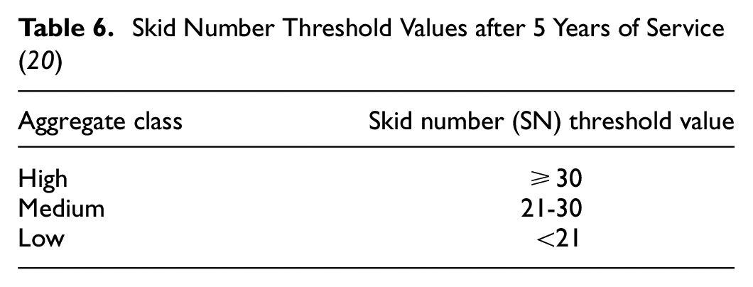
The developed LCC program was utilized to conduct LCCA for the HFST applications based on AIMS, DFT, or BP results. The LCC program was used to predict the NPVs for HFST applications. The NPVs were calculated based on the present and the future costs (maintenance costs) using the inflation and interest rates. Figure 2 shows the calculation process of LCCA. The major input data were categorized into project and material specifics. Details about these inputs are presented in Tables 3 and 4. Three performance prediction models were used to convert the input data into predicted skid number (SN) values, as discussed in the Performance Prediction Models Section. The predicted terminal SN was compared with the recommended or adopted terminal SN based on the rehabilitation matrix as shown in Table 5. This matrix was proposed based on the predicted and recommended terminal SN values. The recommended terminal SN value was controlled by the LCC program user. The recommended terminal SN measured at 50 mph by a skid trailer with smooth tires (SN[50]) was 21 (based on Table 6 [ 20 ]), and the recommended terminal SN measured at 40 mph by a skid trailer with ribbed tires (SN40R) was 40 (based on Table 7 [ 21 ]). If the predicted terminal SN value was greater than or equal to the recommended terminal SN value, then nothing should be done. If the predicted terminal SN value was less than the recommended terminal SN value, then it was recommended to remove the old HFST application and add a new HFST application. Finally, the output data were obtained; these data represented the NPVs for the HFST applications. Based on the lowest NPV, the best HFST application was selected.

Table 3.

Project Specifics Inputs

Input	Value
AADT (vpd)	5,800
Percentage of trucks (%T)	10
Highway classification	Rural
Divided/Undivided highway	Divided
Number of lanes per each direction	2
Lane width (ft)	12
Length of HFST (miles)	1
Cost of removing the HFST ($/yd²)	10
Interest rate (%)	4
Inflation rate (%)	3
Recommended terminal SN(50) value	21
Recommended terminal SN40R	40

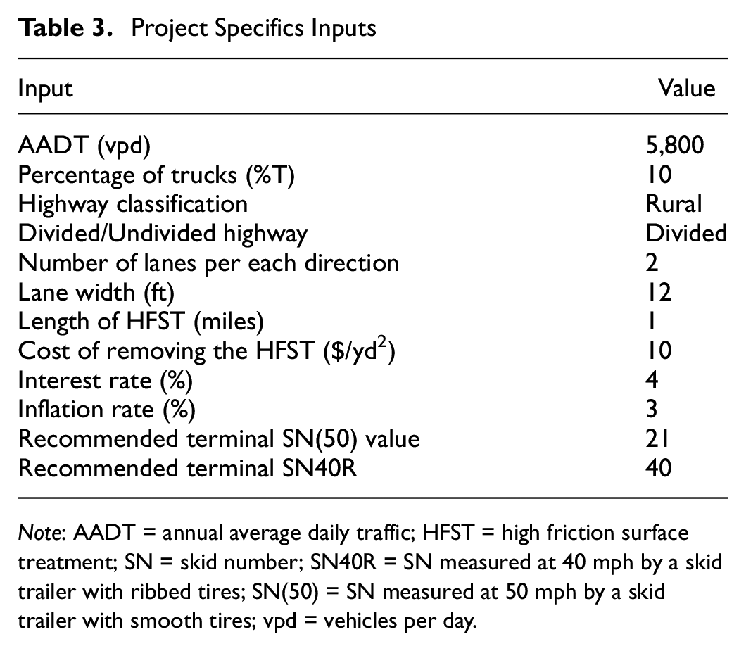
Note: AADT = annual average daily traffic; HFST = high friction surface treatment; SN = skid number; SN40R = SN measured at 40 mph by a skid trailer with ribbed tires; SN(50) = SN measured at 50 mph by a skid trailer with smooth tires; vpd = vehicles per day.

Table 4.

Material Specifics Inputs ( 16 )

Aggregate type	Calcined bauxite	Meramec river aggregate	Earthworks	Rhyolite	Flint	Steel slag
AIMS results
Texture index BMD	318.25	121.35	404.6	370.15	131.25	258.55
Texture index AMD 105	335.15	144.05	318	291.05	124.3	349.4
Texture index AMD 180	303.45	152.5	306.5	288.65	114.65	327.9
Angularity index BMD	2,789.4	2,749.6	3,437.3	3,320.8	2,999.7	3,463.75
Angularity index AMD 105	2,221.35	2,693.1	2,870.6	3,181.55	3,115	3,440
Angularity index AMD 180	2,109.6	2,615.6	2,843.9	3,005.9	3,032.75	3,344.3
DFT results
DFT₄₀ at 0 cycles (initial)	0.95	0.66	0.82	0.81	0.85	0.75
DFT₄₀ at 70k cycles	0.82	0.6	0.62	0.65	0.69	0.67
DFT₄₀ at 140k cycles (terminal)	0.78	0.56	0.55	0.58	0.64	0.63
BP results
BPN before polishing	82.9	80.5	77.5	78.25	78.5	77.5
BPN after polishing	78.9	79	77	73	71.5	76.8
Others
Aggregate cost ($/ton)	575	19.5	300	395	150	2.25
Aggregate transportation distance (mi)	572	121	968	111	250	230
Aggregate shipping cost ($/mi)	3
Number of tons per load	26
Aggregate applied rate (ton/yd²)	0.00675
Epoxy binder cost ($/gallon)	20.50
Epoxy binder shipping cost ($/gallon)	0.16
Epoxy binder applied rate (gallon/yd²)	0.40
Construction, labor, equipment, etc. costs ($/yd²)	5.41

Note: AIMS = aggregate image measurement system; AMD 105 = after 105 min of Micro-Deval (MD) polishing time; AMD 180 = after 180 min of MD polishing time; BMD = before MD polishing; BP = British pendulum; BPN = British pendulum number; DFT₄₀ = coefficient of friction measured using a dynamic friction tester at 40 km/h.

Table 5.

Rehabilitation Matrix for High Friction Surface Treatment (HFST) Applications

What if?	Action
Predicted terminal skid number (SN) ≥ recommended terminal SN	Do nothing
Predicted terminal SN < recommended terminal SN	Remove the old HFST application & add a new HFST application

Table 6.

Skid Number Threshold Values after 5 Years of Service ( 20 )

Aggregate class	Skid number (SN) threshold value
High	≥30
Medium	21-30
Low	<21

Table 7.

Friction Limits for States Based on SN40R ( 21 )

State	SN40R
Illinois	>30
Kentucky	>28
New York	>32
South Carolina	>41
Texas	>30
Utah	>30-35
Washington	>30
Wyoming	>35
Puerto Rico	>40
Maine	>35
Wisconsin	>38

Note: SN40R = skid number measured at 40 mph by a skid trailer with ribbed tires.

Figure 2.

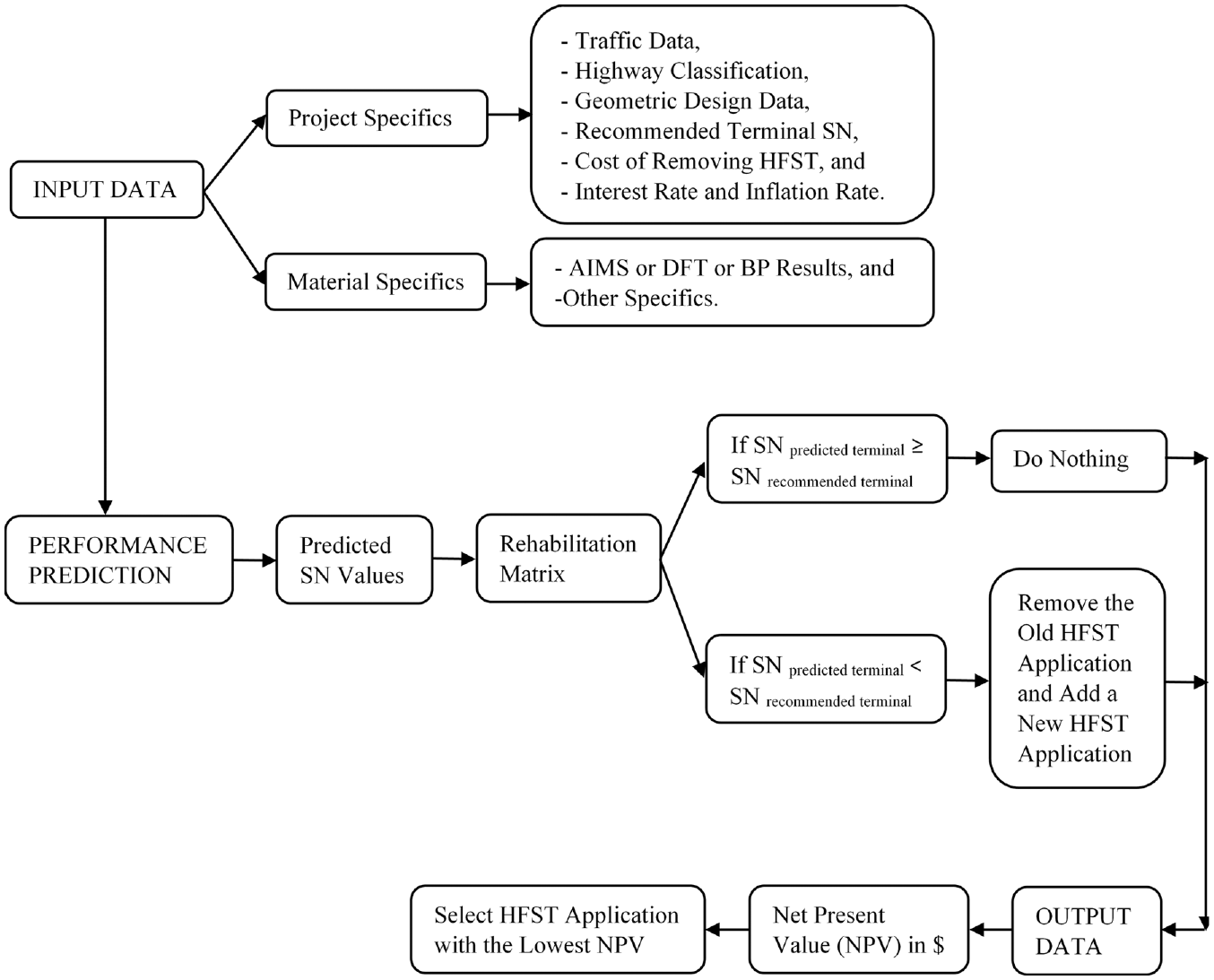
Life cycle cost analysis calculation process.

Input Data

The input data used in the LCC program were organized into two categories: project specifics and material specifics.

Project Specifics

The first data input category was project specifics that included the following:

Traffic data (annual average daily traffic [AADT] per each section in vpd and percentage of trucks [%T]),

Highway classification (rural or urban) and divided or undivided highway,

Geometric design data (number of lanes in each direction, lane width in feet, and the HFST length in miles),

Cost of removing HFST in $/yd²,

The recommended terminal SN(50) and SN40R values, and

Interest rate and inflation rate in %. See Table 3 for the project specifics’ values.

Material Specifics

The material specifics depended on the HFST aggregates’ results (AIMS, DFT, or BP) and other specifics as follows:

Aggregate

Image Measurement System Results

The AIMS results included the texture and angularity indices for before MD polishing (BMD), after 105 min of MD polishing time (AMD 105), and after 180 min of MD polishing time (AMD 180). Table 4 shows AIMS results. Earthworks had the highest texture and angularity indices during BMD polishing, and Meramec River Aggregate presented the lowest texture and angularity indices during BMD polishing. Steel Slag showed the highest texture and angularity indices amid AMD 105 and AMD 180. Flint had the lowest texture indices for AMD 105 and AMD 180, and CB showed the lowest angularity indices for AMD 105 and AMD 180. Texture indices increased using AMD 105 for Meramec River Aggregate, and this increase continued when AMD 180 was used. This happened because the MD polishing exposed a more textured surface that was previously covered by a smoother surface, or the aggregates had mineralogies that exposed new textured surfaces with MD polishing. For CB and Steel Slag aggregates, texture indices increased with AMD 105 and decreased with AMD 180. This occurred because of the breaking of particles, instead of polishing, that exposed their internal surface textures during AMD 105. However, for AMD 180, the polishing process took place on the old and the new exposed internal surface textures. For Earthworks, Flint, and Rhyolite, texture indices decreased for AMD 105 and AMD 180 and reached the lowest values using AMD 180. Angularity indices decreased for all aggregates reaching the lowest value with AMD 180, except for Flint aggregate that had steady values of angularity indices.

Dynamic

Friction Test Results

The DFT results—shown in Table 4—were the DFT₄₀ values measured at three polishing cycles (0, 70k, and 140k cycles). The DFT₄₀ values at zero polishing cycles were considered initial values, and the DFT₄₀ values at 140k polishing cycles represented terminal values. The results showed that the COF decreased with polishing, as expected. CB had higher initial and terminal COF values compared with the other alternative aggregates at the corresponding DFT polishing cycles. The Meramec River Aggregate had the lowest initial friction compared with all other aggregates, and it had comparable terminal friction to that of Earthworks.

British

Pendulum Test Results

The BP results are represented by the BPN values before and after polishing in the British wheel. Note Table 4 for the BP test results. CB had the highest BPN value before polishing followed by Meramec River Aggregate. Meramec River Aggregate showed the highest BPN value after polishing followed by CB. The BPN values before polishing were the same for Earthworks and Steel Slag (77.5). After polishing Earthworks had a higher BPN value than Steel Slag by 0.2. Rhyolite and Flint had comparable average BPN values before polishing; however, Flint showed a lower BPN value after polishing than Rhyolite.

Other Specifics

Aside from the material specifics, the following specifics were taken into consideration:

Aggregate costs in $/ton,

Aggregate shipping costs in $/mile,

Aggregate transportation distance in miles from aggregates’ source to Columbia, MO, U.S.A.,

Number of tons per load (tons/load),

The aggregate applied rate in ton/yd²,

Epoxy binder costs in $/gallon,

Epoxy binder shipping costs in $/gallon,

Epoxy binder applied rate in gallon/yd², and

Construction, labor, equipment, and so forth, costs in $/yd². Table 4 illustrates more details about these input data.

Performance Prediction Models

Three prediction models were used in this study. The first model is presented in Equation 1, the second model is introduced in Equation 7, and the third model is illustrated by Equation 8. The selection of performance prediction models was based on the suitability of the selected materials and performance tests. Equation 1 was used to predict the SN(50) from AIMS texture and angularity indices for BMD, AMD 105, and AMD 180 (20, 22). This model was calibrated based on the results of 31 test sections with seal coat surfaces. Different aggregates were used in the seal coat surfaces (e.g., Limestone, Gravel, Sandstone, Dolomite, and Rhyolite). Equations 2 to 6 depict the steps of calculating the parameters in Equation 1; these equations were calibrated based on the seal coat surfaces’ results (20, 22). Equation 7 aimed to predict the SN40R from the DFT₄₀ before and after polishing. This model was developed by Heitzman et al. ( 3 ) for three HFST applications using Granite, Flint, and CB. Equation 8 correlated the BP results and SN40R ( 23 ). This model was developed based on 23 test sections of dense-graded asphalt concrete, open-graded asphalt concrete, and Portland cement concrete ( 23 ). However, it was used in this study for HFST applications’ comparison purposes only.

Prediction Model Based on Aggregate Image Measurement System Test Results

The AIMS results were used to predict the SN for the HFST applications based on a SN prediction model developed for seal coats (20, 22). Based on this model, the relationship between the SN(50) and international friction index (IFI) was developed as presented in Equation 1. The IFI prediction model for the seal coat is shown in Equation 2.

SN (50) = 4.81 + 140.32 (IFI - 0.045) e^{- 20 / S_{p}}

(1)

where

S_p is the speed constant parameter ( $S_{p} = 14.2 + 89.7 MPD$ ), and

MPD is the mean depth profile ( $MPD = (λ / 5.403) + (3.491 / κ) + κ^{0.104} + N^{- 0.47} - 2.594$ ),

$λ$ and $κ$ are scale and shape parameters of the Weibull distribution, respectively. These parameters were obtained by fitting Equation 3 (9, 24 –26) and changed according to the aggregates’ gradations, and

N is the number of polishing cycles in the laboratory, using the TWPD, in thousands (e.g., N = 10 for 10,000 polishing cycles). It was calculated using Equation 4.

IFI (N) = a_{mix} + b_{mix} \times e^{(- {c_{m}}_{ix} \times N)}

(2)

where

a_mix is the terminal IFI ( $a_{mix} = \frac{40.493 + λ}{330 - 0.0011 {(AM D_{TX})}^{2}}$ ),

(a_mix+b_mix) is the initial IFI ( $a_{mix} + b_{mix} = 0.4 \times \ln (\frac{1.43757 \times (a_{TX} + b_{TX}) + 46.8933 \times λ + 3343.491 \times κ}{2.02031 \times (a_{GA} + b_{GA})})$ ),

c_mix is the rate of change in IFI ( $c_{m i x} = 2.654 \times c_{T X} + 1.5 \times c_{G A}$ ),

AMD_TX is the aggregate texture—measured by the AIMS—after 105 min of polishing in the MD device,

The $a_{TX}$ , $b_{TX}$ , and $c_{TX}$ were texture regression constants and obtained from Equation 5, and

the $a_{GA}$ , $b_{GA}$ , and $c_{GA}$ were angularity regression constants and obtained from Equation 6.

F (x, λ, κ) = 1 - e^{- (\frac{X}{λ})} κ

(3)

where

F is the cumulative percentage passing, and

x is the aggregate size in mm.

N = TMF \times 10^{(\frac{1}{A + B \times c_{mix} + (\frac{C}{c_{mix}})})}

(4)

where

TMF is the traffic multiplication factor ( $TMF = \frac{Days between construction and field testing \times Adjusted traffic}{1000}$ ),

A, B, and C are regression coefficients (A = −0.452, B = −58.95, and C = 5.834 $\times 10^{- 6}$ ),

$Adjusted traffic = \frac{AADT \times (100 - % T) \times DL F_{AADT}}{100} + \frac{AADT \times (% T) \times DL F_{T}}{100}$ ,

AADT is the annual average daily traffic for each section,

%T is the percentage of trucks,

$Dl f_{AADT}$ is the design lane factor of AADT (depending on the number of lanes and highway classification [urban or rural]), and

$Dl f_{T}$ is the design lane factor of trucks (depending on the number of lanes and highway classification [urban or rural]). The $Dl f_{AADT}$ and $Dl f_{T}$ values are presented in Table 8.

Table 8.

Design Lane Factors of Annual Average Daily Traffic (AADT) and Trucks ( 20 )

Number of lanes per each direction	Rural highway				Urban highway
	Undivided		Divided		Undivided		Divided
	$Dl f_{AADT}$	$Dl f_{T}$	$Dl f_{AADT}$	$Dl f_{T}$	$Dl f_{AADT}$	$Dl f_{T}$	$Dl f_{AADT}$	Dlf_T
1	0.50	0.50	NA	NA	0.50	0.50	NA	NA
2	0.40	0.45	0.80	0.90	0.30	0.40	0.70	0.90
3	0.30	0.40	0.40	0.50	0.25	0.35	0.40	0.50
4	NA	NA	NA	NA	NA	NA	0.30	0.40

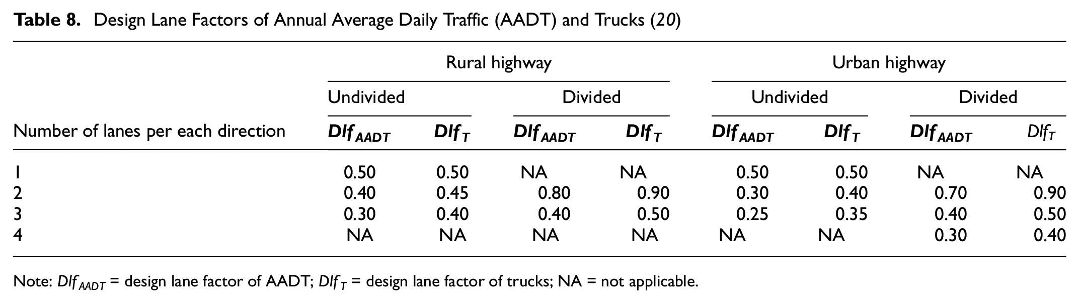
Note: $Dl f_{AADT}$ = design lane factor of AADT; $Dl f_{T}$ = design lane factor of trucks; NA = not applicable.

Equation 5 illustrates the relationship between the change in the texture index and the MD polishing time (t) in minutes. The regression constants were obtained by fitting three texture measurements with AIMS: BMD, AMD 105, and AMD 180 (9, 25, 27, 28).

TX (t) = a_{TX} + b_{TX} \times e^{(- c_{TX} \times t)}

(5)

where

TX is the texture index measured by AIMS,

t is the MD polishing time,

$a_{TX}$ is the terminal texture index,

( $a_{TX}$ + $b_{TX}$ ) is the initial texture index, and

$c_{TX}$ is the rate of texture change.

Equation 6 presents the relationship between the change of aggregate angularity index and the MD polishing time (t). The regression constants were obtained by fitting the three angularity measurements by AIMS: BMD, AMD 105, and AMD 180 (9, 25, 27, 28).

GA (t) = a_{GA} + b_{GA} \times e^{(- c_{GA} \times t)}

(6)

where

GA is the angularity index measured by AIMS,

t is the MD polishing time,

$a_{GA}$ is the terminal angularity index,

( $a_{GA}$ + $b_{GA}$ ) is the initial angularity index, and

$c_{GA}$ is the rate of angularity change.

Prediction Model Based on Dynamic Friction Test Results

The DFT₄₀ values—at different polishing cycles—were used to predict the SN40R. The initial SN40R was calculated at zero polishing cycles; the terminal SN40R was calculated at 140k polishing cycles. Heitzman et al.’s model was used in this study to compare the different HFST applications. This model was based on laboratory friction measurements using DFT₄₀ and SN40R in the field for three HFST applications ( 3 ). The friction limits differed from one state to another. Table 7 presents the friction limits for states based on the SN40R values ( 21 ). Equation 7 explains the relationship between the SN40R and the DFT₄₀:

SN 40 R = 92.3 \times DF T_{40} - 13.9

(7)

where

SN40R is the predicted SN measured in the field using a skid trailer with ribbed tires at 40 mph, and

DFT₄₀ if the COF values measured by DFT at 40 km/h in the lab.

Prediction Model Based on British Pendulum Test Results

The BP results for aggregates’ coupons were used to predict the SN40R. The relationship between the BPN and the SN40R is presented in Equation 8 ( 23 ):

SN 40 R = 0.83 (BPN) - 10.5

(8)

where

SN40R is the SN measured at 40 mph by a skid trailer with ribbed tires, and

BPN is the British pendulum number.

The user interface of the LCC program is shown in Figure 3. The user interface included three buttons on the upper right side: the first was for AIMS, the second was for BP, and the third was for DFT. These buttons reflected different Excel sheets with different material specifics and prediction models. The user can transfer from one sheet to another based on the available data (e.g., AIMS, BP, or DFT). For AIMS material specifics, once the program user has entered the AIMS texture and angularity indices, the Run AIMS Optimization button must be pressed. The Excel sheet’s buttons were designed using Visual Basic coding.

Figure 3.

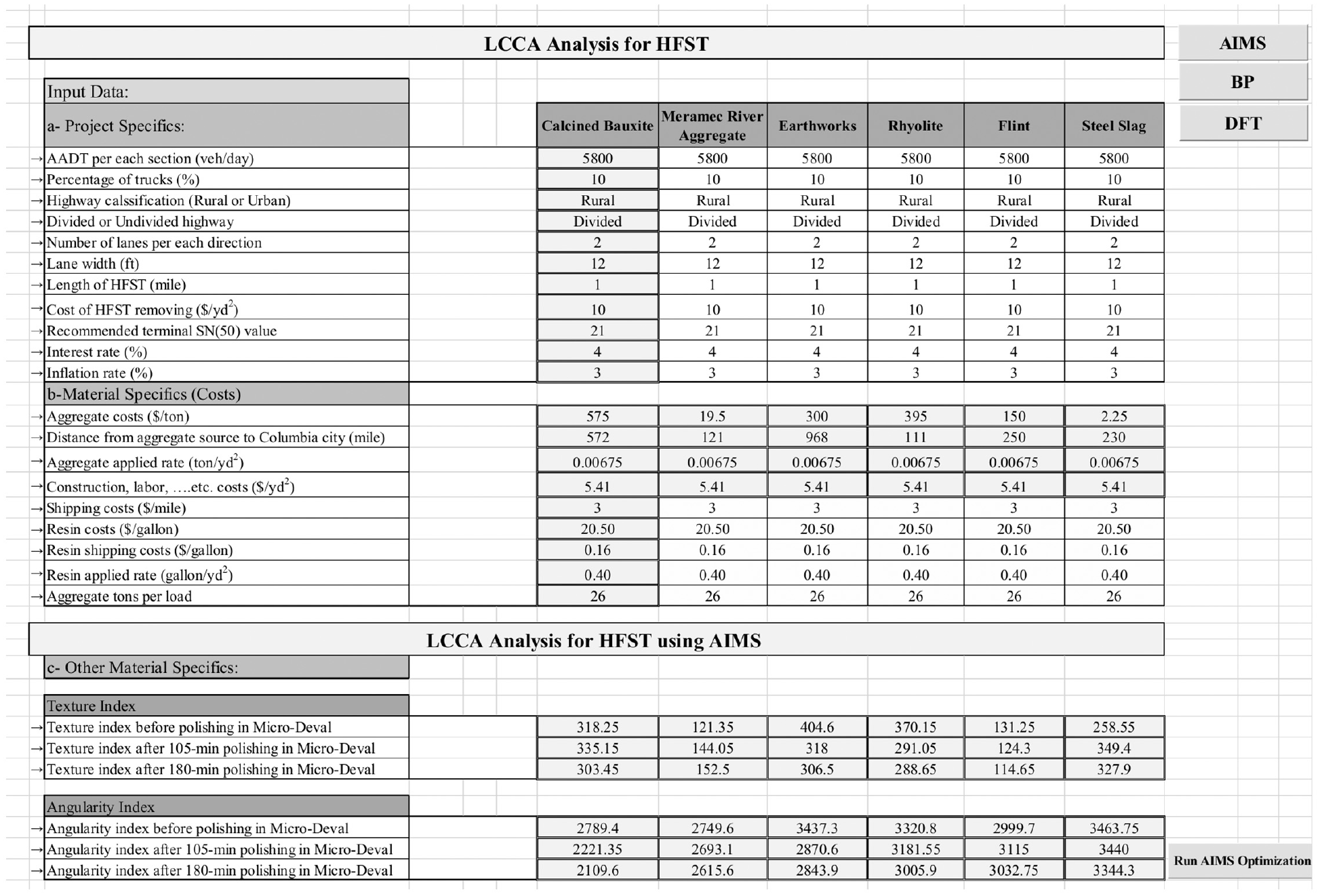
Life cycle cost program user interface.

LCCA Results

The following subsections discussed the LCCA analysis results—obtained from the LCC program—based on the AIMS, DFT, and BP input data. After, a comparative LCCA study was conducted to select the appropriate HFST application based on the NPV obtained from LCCA studies.

Skid Number

Figure 4a displays the predicted initial SN(50) values and SN(50) values after 5 years of service—deemed terminal—based on AIMS input data for HFST applications. The SN(50) values decreased after 5 years of service. CB HFST application had the highest initial SN(50) followed by Meramec River Aggregate HFST application and then Flint HFST application; Steel Slag HFST application had the lowest value. Flint HFST application presented the highest terminal SN(50) value followed by Meramec River Aggregate HFST application and then CB HFST application; Steel Slag HFST application yielded the lowest value. Based on the initial and terminal SN(50) values, Steel Slag had the lowest polishing process resistance. By contrast, Flint presented the highest resistance to the polishing process.

Figure 4.

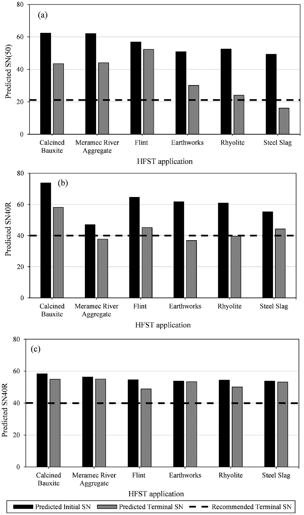
Predicted initial and terminal skid number values for HFST applications: (a) based on AIMS, (b) based on DFT₄₀, and (c) based on BP.

Figure 4b illustrates the predicted SN40R based on DFT₄₀ input data initially (0 polishing cycles) and terminally (after 140k polishing cycles) for HFST applications. The polishing process using TWPD decreased the SN40R values. CB HFST application displayed the highest initial and terminal SN40R values followed by Flint HFST application. Meramec River Aggregate HFST application had the lowest initial SN40R value, and Earthworks HFST application had the lowest terminal SN40R value. Earthworks HFST application had a higher initial SN40R value than Meramec River Aggregate HFST application; however, the terminal SN40R values for both HFST applications were comparable. Earthworks and Rhyolite HFST applications presented higher initial SN40R values than Steel Slag HFST application yielded. Nevertheless, Steel Slag HFST application had higher terminal SN40R values than Earthworks and Rhyolite HFST applications. Moreover, Steel Slag and Flint had comparable terminal SN40R values.

Figure 4c depicts the predicted initial and terminal SN40R based on the BP input data for the HFST applications. The British wheel polishing process decreased the SN40R values. CB HFST application had the highest initial SN40R value, and Meramec River Aggregate HFST application had the highest terminal SN40R value. Flint HFST application had the lowest terminal SN40R followed by Rhyolite HFST application. Steel Slag and Earthworks HFST applications had similar SN40R values: the initial SN40R value was 53.83 for both applications, the terminal SN40R value was 53.41 for Earthworks application, and the terminal SN40R value was 53.20 for Steel Slag application.

Net Present Value

The NPVs for the HFST applications based on AIMS input data are shown in Figure 5a. The best choice was the HFST application using Meramec River Aggregate because it had the lowest NPV at $98,380. The second-best choice was the Flint HFST application with a NPV of $104,764. Earthworks and Rhyolite HFST applications had comparable NPVs. The worst choice was the HFST application using Steel Slag; it had a NPV of $259,296. CB HFST application had the second highest NPV after Steel Slag HFST application. The high NPV for the CB HFST application occurred because of its high cost: CB showed the highest cost (575 $/ton) when compared with the alternative aggregates’ costs. However, the Steel Slag HFST application showed the highest NPV because it had the lowest terminal SN(50), see Figure 4b, and this value was lower than the recommended terminal SN value. Additionally, the HFST application using Steel Slag was the only application that required replacement after 5 years of service.

Figure 5.

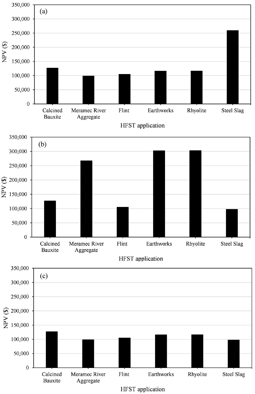
Net present values for HFST applications: (a) based on AIMS, (b) based on DFT₄₀, and (c) based on BP.

The NPVs for the HFST applications based on DFT₄₀ input data are shown in Figure 5b. The best choice was the HFST application using Steel Slag because it had the lowest NPV at $97,633. This occurred because Steel Slag had the lowest cost (2.25 $/ton), and no HFST replacement was required when it reached the terminal SN40R value. The second-best choice was the Flint HFST application with a NPV of $104,764. Flint HFST application had the third-lowest cost after Steel Slag and Meramec River Aggregate. When the HFST applications reached their terminal SN40R values, no replacement took place for the HFST application using Flint, and replacement happened for the HFST application using Meramec River Aggregate. Thus, the HFST application using Flint had a lower NPV than the HFST application using Meramec River Aggregate. CB HFST application was the third choice with a NPV of $126,725. CB had the highest cost between the aggregates; however, no HFST application replacement happened when it reached the terminal SN40R value. Furthermore, the CB HFST application had the highest terminal SN40R value (see Figure 4b). Earthworks and Rhyolite HFST applications were the worst choices because they showed the highest NPVs (more than $302,000) followed by Meramec River Aggregate HFST application with a NPV of $267,159. Earthworks and Rhyolite had costs lower than CB and higher than the remaining aggregates. Moreover, HFST applications using Earthworks or Rhyolite HFST applications required replacement when they reached the terminal values.

Figure 5c exhibits the NPVs for the HFST applications based on the BP input data. Figure 5c exemplified the lowest NPVs when compared with Figure 5, a and b. This took place because no HFST application replacement happened when the aggregates reached the terminal SN40R values. The best choice was the HFST application using Steel Slag because it had the lowest NPV valued at $97,633. Steel Slag had the lowest cost, and no HFST application replacement happened when they reached the terminal SN40R values. The second-best choice was the Meramec River Aggregate HFST application with a NPV of $98,380 followed by Earthworks HFST application with a NPV of $115,828. CB HFST application was the worst choice because it presented the highest NPV ($126,725) followed by Rhyolite HFST application with a NPV of $116,223.

Comparative LCCA Study

In this section, the NPV data obtained from the LCC program were compared for the HFST applications. The NPV ranked 1 to 6. The HFST application with the lowest NPV ranked 1, and the HFST application with the highest NPV ranked 6. Table 9 presents the rankings based on NPV. HFST applications’ rankings were considered high at 1 or 2, moderate at 3 or 4, and low at 5 or 6. CB, Earthworks, and Rhyolite HFST applications’ rankings were between moderate and low. Steel Slag HFST application’s rankings were between high and low. Flint and Meramec River Aggregate HFST applications’ rankings were considered between high and moderate.

Table 9.

Ranking of HFST Applications

HFST application	Ranking of NPV
HFST application	AIMS	DFT₄₀	BP
Calcined bauxite	5	3	6
Earthworks	3	5	4
Rhyolite	4	6	5
Flint	2	2	3
Steel slag	6	1	1
Meramec river aggregate	1	4	2

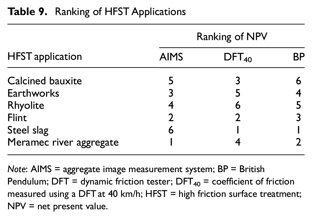
Note: AIMS = aggregate image measurement system; BP = British Pendulum; DFT = dynamic friction tester; DFT₄₀ = coefficient of friction measured using a DFT at 40 km/h; HFST = high friction surface treatment; NPV = net present value.

Comparative cost analysis for HFST applications was executed based on two scenarios. The first scenario represented HFST applications without a maintenance action, note Figure 6a. The second scenario, presented in Figure 6b, was proposed based on a maintenance action for HFST applications. The maintenance action involved removing the old HFST application and applying a new HFST application, note Table 5. For both scenarios, cost percentages were calculated by dividing each cost by the total cost. The costs included the cost of removing the HFST, the aggregate cost, the aggregate shipping cost, the resin cost, the resin shipping cost, and construction and labor costs. For the first scenario, Figure 6a, the cost of resin dominated the total cost of HFST application followed by construction and labor costs and then the aggregate cost. The resin cost was between 46% and 59% of the total cost of the HFST application. Construction and labor costs were between 30% and 39% of the total cost of the HFST application. The aggregate costs were between 0.11% for Steel Slag and 22% for CB when compared with the total cost of HFST application. Aggregate shipping costs were less than 5% of the total cost of the HFST application, and the resin shipping cost was less than 0.5% of the total cost of the HFST application. Shipping costs mainly depended on the distance between the material origin and the destination. Thus, Earthworks aggregate’s shipping cost was the highest because the distance between Earthworks aggregate’s origin and the destination was the longest. For the second scenario, Figure 6b, resin cost controlled the total cost of HFST application followed by construction and labor costs, the HFST removal cost, and then the aggregate cost. The resin cost was between 36% and 44% of the total cost of the HFST application. Construction and labor costs ranged from 24% to 29% of the total cost of the HFST application. The cost of HFST removal was between 22% and 27% of the total cost of HFST application. The aggregate costs were between 0.08% for Steel Slag and 17% for CB as compared with the total cost of HFST application. Aggregate shipping costs were less than 2% of the total cost of the HFST application, and the resin shipping cost was less than 0.5% of the total cost of the HFST application.

Figure 6.

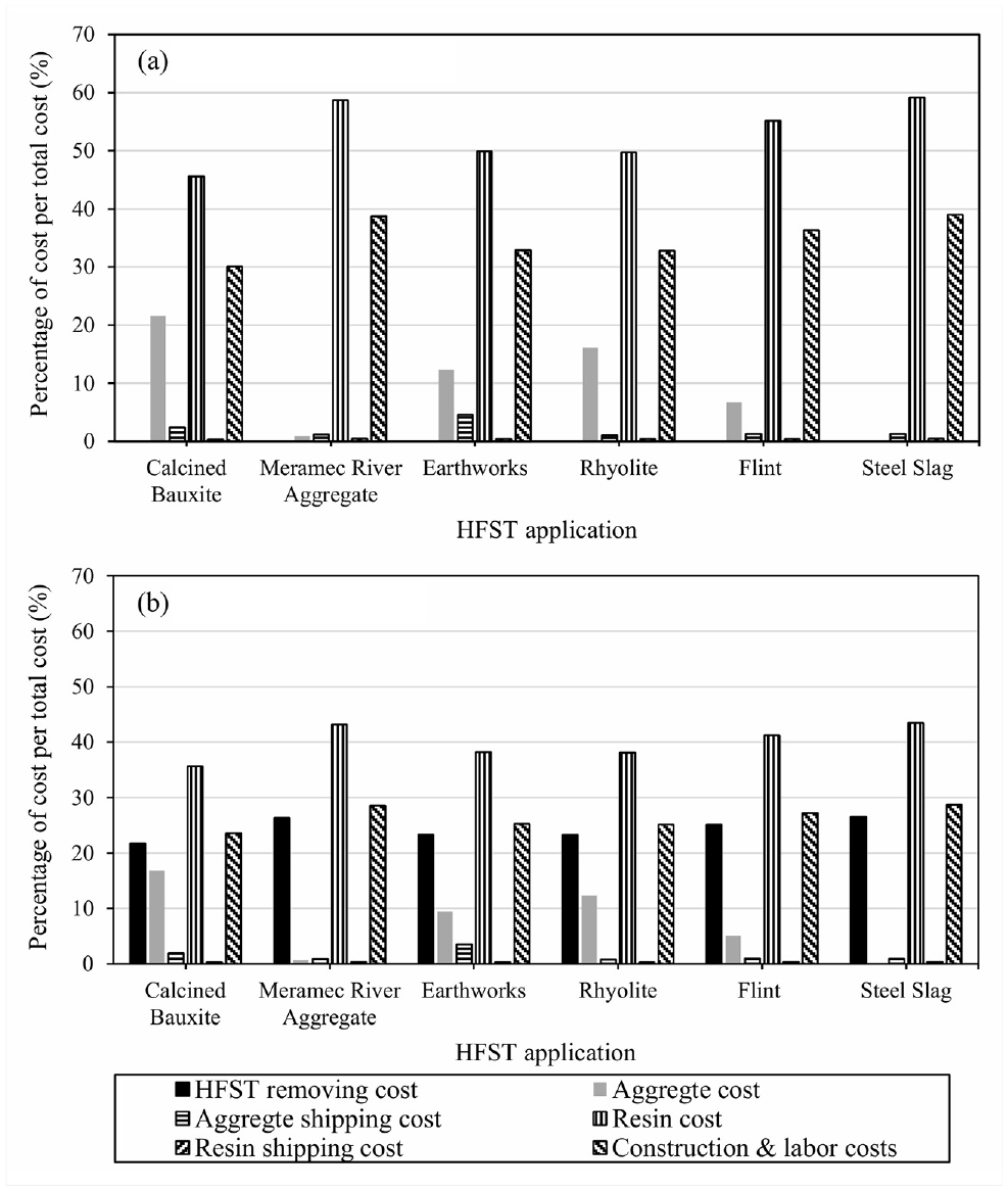
Comparative cost analysis for high friction surface treatment (HFST) applications: (a) no maintenance applied and (b) maintenance applied.

Conclusions and Recommendations

In this study, the LCCAs of HFST applications using CB and five CB alternatives were discussed. The CB alternatives were Earthworks, Meramec River Aggregate, Flint, Steel Slag, and Rhyolite. The performances of the aggregates were analyzed using an AIMS. The performance of the HFST applications was evaluated by DFT and BP. The researchers developed a simple LCC program using Microsoft Excel to predict the NPV for the HFST applications. The primary purpose of this LCC program was to present a rational method for converting different input data (project and material specifics) into comparable output data (NPV) that facilitated comparison among different alternatives. Three prediction models were utilized to convert the performance testing results to SN values: the first model was based on AIMS results, the second model correlated the DFT results and SN, and the third model linked the BP results to SN. The first prediction model was validated for seal coats and similar aggregates used here (e.g., Rhyolite). The second prediction model was developed for the HFST application. However, the third prediction model was based on flexible and rigid pavement sections. The predicted terminal SN values for the HFST applications were compared with the recommended terminal SN values and could be adopted by the LCC program’s user. The decision for maintenance of the HFST was taken using a rehabilitation matrix. By analyzing the LCC program output data, the following points were concluded and recommended:

The LCC analysis based on the BP results had similar results to the LCC analysis based on the DFT results (e.g., Steel Slag was the best alternative to CB).

The LCC analysis based on AIMS had different results when compared with the LCC analysis based on the BP or DFT because the BP and DFT tests evaluated the aggregates’ surface frictional properties directly. However, the AIMS reflected the frictional properties through indirect measurements (e.g., changes occurred in the texture and angularity indices after the MD polishing).

For any performance prediction model, the aggregate source controlled the NPV results.

Resin cost dominated the total cost of the HFST application followed by construction and labor costs, HFST removal cost, and then aggregate cost.

Meramec River Aggregate and Flint HFST applications had the lowest NPVs followed by Steel Slag HFST application and then Earthworks HFST application. By contrast, the Rhyolite HFST application showed the highest NPVs followed by the CB HFST application.

It is recommended to use Meramec River Aggregate, Flint, and Steel Slag as CB alternatives.

Adopting the developed LCC program as a rational tool to compare the aggregate source alternatives for HFST applications is recommended.

Footnotes

Acknowledgements

The authors acknowledge the technical and funding support of MoDOT for providing instruments and information for this research. The dynamic friction test was conducted at the University of Idaho under the supervision of Dr. Emad Kassem and Mr. Juan Pinto Ortiz.

Author Contributions

The authors confirm contribution to the paper as follows: study conception and design: M. Abdelrahman and E. Deef-Allah; data collection: M. Abdelrahman, E. Deef-Allah, and Korrenn Broaddus; analysis and interpretation of results: E. Deef-Allah and M. Abdelrahman; draft manuscript preparation: E. Deef-Allah and M. Abdelrahman. All authors reviewed the results and approved the final version of the manuscript.

Declaration of Conflicting Interests

The author(s) declared no potential conflicts of interest with respect to the research, authorship, and/or publication of this article.

Funding

The author(s) disclosed receipt of the following financial support for the research, authorship, and/or publication of this article: This work was funded by the Missouri Department of Transportation (MoDOT).

ORCID iDs

Eslam Deef-Allah

Korrenn Broaddus

Magdy Abdelrahman

Data Accessibility Statement

The data used in this study may be made available on reasonable request to the corresponding author.

References

FHWA-CAI-14-019. Frequently Asked Questions About High Friction Surface Treatments (HFST). FHWA. n.d. https://www.fhwa.dot.gov/innovation/everydaycounts/edc-2/pdfs/fhwa-cai-14-019_faqs_hfst_mar2014_508.pdf. Accessed March 9, 2021.

FHWA. High Friction Surface Treatment (HFST) Quick Reference. DTFH61-13-D-00001, Task B9. 2020. https://www.fhwa.dot.gov/publications/research/safety/highfriction/High-Friction-Surface-Treatment-final.pdf. Accessed March 3, 2021.

Heitzman

Turner

Greer

NCAT Report 15-04: High Friction Surface Treatment Alternative Aggregates Study. National Center for Asphalt Technology at Auburn University, Auburn, AL, 2015.

Heitzman

Moore

NCAT Report 17-01: Evaluation of Laboratory Friction Performance of Aggregates for High Friction Surface Treatments. National Center for Asphalt Technology at Auburn University, Auburn, AL, 2017.

Wilson

Mukhopadhyay

Final Report: Alternative Aggregates and Materials for High Friction Surface Treatments. Project BDR74-977-05. Texas A&M Transportation Institute, College Station, TX, 2016.

Merritt

Moravec

Heitzman

High Friction Surface Treatment Aggregate Durability Study. Pavement Evaluation 2014, Blacksburg, VA, 2014. https://vtechworks.lib.vt.edu/bitstream/handle/10919/54620/Merritt.pdf?sequence=1&isAllowed=y. Accessed March 9, 2021.

Milstead

Qin

Katz

Bonneson

Pratt

Miles

Carlson

FHWA-SA-11-22: Procedures for Setting Advisory Speeds on Curves. Federal Highway Administration, Office of Safety, Washington, D.C., 2011.

Bloem

D. L.

Skid Resistance: The Role of Aggregates and Other Factors. National Sand and Gravel Association Circular 109, Silver Spring, MD, 1971.

Kassem

Awed

Masad

E. A.

Little

D. N.

Development of Predictive Model for Skid Loss of Asphalt Pavements. Transportation Research Record: Journal of the Transportation Research Board, 2013. 2372: 83–96.

10.

Kandhal

P. S.

Parker

NCHRP Report 405: Aggregate Tests Related to Asphalt Concrete Performance in Pavements. Transportation Research Board, National Research Council, Washington, D.C., 1998.

11.

Crouch

L. K.

Gothard

J. D.

Head

Goodwin

W. A.

Evaluation of Textural Retention of Pavement Surface Aggregates. Transportation Research Record: Journal of the Transportation Research Board, 1995. 1486: 124–129.

12.

Fuentes

L. G.

Gunaratne

de León Izeppi

Flintsch

G. W.

Martinez

Determination of Pavement Macrotexture Limit for Use in International Friction Index Model. Transportation Research Record: Journal of the Transportation Research Board, 2012. 2306: 138–143.

13.

Kubba

Green Design and Construction Economics. In Green Construction Project Management and Cost Oversight ( Kubba

, ed.), Architectural Press, Oxford; Burlington, MA, 2010, pp. 304–342. https://doi.org/10.1016/B978-1-85617-676-7.00008-7.

14.

Kendall

Keoleian

G. A.

Helfand

G. E.

Integrated Life-Cycle Assessment and Life-Cycle Cost Analysis Model for Concrete Bridge Deck Applications. Journal of Infrastructure Systems, Vol. 14, 2008, pp. 214–222. https://doi.org/10.1061/(ASCE)1076-0342(2008)14:3(214).

15.

Walls

III Smith

M. R.

FHWA-SA-98-079: Life-Cycle Cost Analysis in Pavement Design—Interim Technical Bulletin. Federal Highway Administration, Washington, D.C., 1998.

16.

Deef-Allah

Broaddus

Abdelrahman

cmr21-006: Evaluation of Alternatives to Calcined Bauxite for Use in High Friction Surface Treatment (HFST) in Missouri, Missouri University of Science and Technology, MO, 2021.

17.

Xiong

Cong

Shah

Jiang

Laboratory Evaluation of Critical Properties and Attributes of Calcined Bauxite and Steel Slag Aggregates for Pavement Friction Surfacing. Journal of Materials in Civil Engineering, Vol. 31, No. 8, 2019, p. 04019155. https://doi.org/10.1061/(ASCE)MT.1943-5533.0002806.

18.

Xiong

Zhao

Cong

Jiang

FHWA/IN/JTRP-2017/09: Friction Surface Treatment Selection: Aggregate Properties, Surface Characteristics, Alternative Treatments, and Safety Effects. Joint Transportation Research Program Purdue University West Lafayette, IN, 2017. https://doi.org/10.5703/1288284316509.

19.

IDOT. 2018 Standard Specifications for Highway Construction. IDOT, Boise, ID, 2018.

20.

Chowdhury

Kassem

Aldagari

Masad

Technical Report 0-6746-01-1: Validation of Asphalt Mixture Pavement Skid Prediction Model and Development of Skid Prediction Model for Surface Treatments. Texas A&M Transportation Institute, College Station, TX, 2016.

21.

Henry

J. J.

NCHRP Synthesis 291: Evaluation of Pavement Friction Characteristics: A Synthesis of Highway Practice. Transportation Research Board–National Research Council, Washington, D.C., 2000.

22.

Aldagari

Al-Assi

Kassem

Chowdhury

Masad

Development of Predictive Models for Skid Resistance of Asphalt Pavements and Seal Coat. International Journal of Pavement Engineering, 2020, pp. 1–13. https://doi.org/10.1080/10298436.2020.1766685.

23.

Henry

J. J.

Wambold

J. C.

Use of Smooth-Treaded Test Tire in Evaluating Skid Resistance. Transportation Research Board: Journal of the Transportation Research Board, 1992. 1348: 35–42.

24.

Masad

Rezaei

Chowdhury

Harris

FHWA/TX-09/0-5627-1: Predicting Asphalt Mixture Skid Resistance Based on Aggregate Characteristics. Texas Transportation Institute, Texas A&M University, College Station, TX, 2009.

25.

Masad

Luce

Mahmoud

FHWA/TX-06/5-1707-03-1: Implementation of AIMS in Measuring Aggregate Resistance to Polishing, Abrasion, and Breakage. Texas Transportation Institute, Texas A&M University, College Station, TX, 2006.

26.

Masad

Rezaei

Chowdhury

FHWA/TX-11/0-5627-3: Field Evaluation of Asphalt Mixture Skid Resistance and its Relationship to Aggregate Characteristics. Texas Transportation Institute, Texas A&M University, College Station, TX, 2011.

27.

Mahmoud

E. M.

Development of Experimental Methods for the Evaluation of Aggregate Resistance to Polishing, Abrasion, and Breakage. M.Sc. thesis. Texas A&M University, College Station, TX, 2005.

28.

Mahmoud

Masad

Experimental Methods for the Evaluation of Aggregate Resistance to Polishing. Abrasion, and Breakage. Journal of Materials in Civil Engineering, Vol. 19, 2007, pp. 977–985. https://doi.org/10.1061/(ASCE)0899-1561(2007)19:11(977).