Design Method of Worn Rail Grinding Profile for the Curve Section

Abstract

The grinding profile directly affects the wheel–rail contact relationship, so it is necessary to study the design method of rail grinding profiles for the curve section. Based on the Frechet distance method, the selection method of representative profile for worn rails was established. Based on the non-uniform rational B-spline theory, the description model of the rail profile was constructed. The reduction of rail grinding material removed and improvement of wheel–rail contact geometry were taken as the optimization objectives, and the multi-objective function of the grinding profile of the outer rail in the transition curve and circular curve section was established. The optimized design results show that compared with the measured grinding profile in the field, the rail grinding amount is reduced by 80.1% and 11.3% by using grinding profiles designed for the transition curve section and the circular curve section, respectively, and the distribution of wheel–rail contact points is more uniform. The dynamic indexes under different velocities and different radii are significantly reduced, and the curve passing performance is improved. The area of wheel–rail contact spot changes uniformly with the lateral displacement of the wheelset, and the maximum von Mises stress is improved obviously. The wear index and surface fatigue index decreased significantly. The optimized grinding profile can effectively extend the maintenance cycle and service life of the curved rail.

Keywords

rail freight rail transportation heavy rail safety

With the rapid development of the railway, the area of the railway network is expanding and the mileage of the railway operation is extending. Moreover, there are many curve sections in railway lines. The wheel–rail relationship in this area is complex, and the problem of rail wear is prominent. Unreasonable matching of wheel–rail profiles is an important factor that causes the increase of rail wear in the curve section. At present, the main measure to reduce rail wear is rail grinding, and the grinding target profile is the key to determining the grinding quality.

Scholars at home and abroad have done a great deal of research on profile optimization design. Smallwood et al. ( 1 ) found that wheel–rail contact stress was the main factor affecting the initiation and propagation of rolling contact fatigue crack. Taking the reduction of wheel–rail contact stress as the optimization objective, the design profile significantly reduced the contact stress compared with the British standard profile, and maintained its good dynamic performance. Brandau ( 2 ) optimized the profiles of inner and outer rails by controlling the coordinates of finite discrete points on the railhead, and realized the asymmetric design of the curved rail. Persson et al. ( 3 ) established a nonlinear mathematical model of the rail profile and dynamic performance parameters, and obtained the optimized profile based on a genetic algorithm. The actual test showed that the rail profile effectively alleviated contact fatigue and reduced rail wear. Choi et al. ( 4 ) proposed the optimization method of the rail profile with the reduction of the rail wear index as the objective function to solve the abnormal rail wear phenomenon in the process of subway operation. The relevant parameters of dynamics were used as the constraint function. The optimization results show that the optimized profile can significantly reduce the rail wear caused by the running process of subway vehicles.

To reduce railhead wear on the working side, Zong and Dhanasekar ( 5 , 6 ) changed the formulation of the railhead shape into a multivariable optimization problem, and the optimized profile was obtained based on the finite element method and genetic algorithm with the optimization goal of minimizing contact stress. Taking the rail wear rate as the objective function, Wang et al. ( 7 ) used the support vector machine regression theory to fit the nonlinear relationship between the rail profile and the wear rate, and obtained the optimized profile through the genetic algorithm. As a result, the wear rate of the optimized rail was significantly reduced. To modify the rail pre-grinding profile smoothly, Zheng et al. ( 8 ) parameterized the profile by using the non-uniform rational B-spline (NURBS) curve, and obtained the optimized profile based on the non-dominated sorting genetic algorithm. Jiang and Gao ( 9 ) proposed an optimization scheme of the rail profile based on the coupling method of the artificial neural network and genetic algorithm. The optimized rail not only reduced the rail wear rate, but also maintained a good dynamic performance and wheel–rail contact state. Huang ( 10 ) proposed an optimization design method of the rail grinding profile based on the analysis of wheel–rail contact stress, and verified the feasibility of this method by comparing the wheel–rail contact geometric performance and contact stress before and after optimization. Lin et al. ( 11 , 12 ) proposed a smooth design method for constructing a rail profile with multi-parameter variables, such as a multi-section arc and radius, and then established a cubic NURBS description method for the rail profile based on NURBS theory, and obtained the optimized profile through the optimization algorithm. Zhou ( 13 ) adopted the reverse method of the wheel–rail contact angle curve to design a rail profile with high commonness, which effectively improved the wheel–rail contact state. Mao and Shen ( 14 ) deduced the rail grinding profile directly by designing the wheel diameter difference function, which can meet different grinding requirements by adjusting the wheel diameter difference and expected contact distribution. Tang et al. ( 15 ) established a multi-objective optimization design method for the rail profile based on the genetic algorithm and analytic hierarchy process, and the wheel–rail contact analysis showed that the optimized profile was very effective in reducing wheel–rail wear and contact stress. Considering the wear characteristics and wheelset dynamics of linear rail, Wang ( 16 ) took the highest wheel–rail conformality at the wheel–rail contact point as the objective function, parameterized the rail profile, and proposed a rail profile optimization design algorithm based on the series quadratic programming (SQP) algorithm. Wang ( 17 ) optimized the profile of the key section of the rail in the crossing zone based on particle swarm optimization, and the surface fatigue index of the designed profile was significantly reduced, which effectively reduced the fatigue damage of the rail in the crossing zone.

The above research obtained optimized rail profiles from different perspectives, which effectively improved the wheel–rail contact relationship and dynamic performance. However, at present, the optimized profile is mostly a single rail grinding target profile; without considering the influence of the curvature change of the curve section on the rail wear, the grinding mode adopted in the entry and exit transition curve section is consistent with the circular curve section. The traditional method mostly relies on the use of a single target profile for the grinding operation, resulting in large grinding errors and grinding costs. At the same time, the optimized design profile is mostly based on the maximum worn profile, which cannot represent the overall wear of the whole section. The domestic and foreign research summary and the technical route of this paper are shown in Figure 1. The paper is based on measured rail profiles of a heavy-haul railway in the curve section. The Frechet distance method is used to select the representative profile of the worn rails in different sections. Based on the NURBS curve theory, worn rail profiles in the transition curve section and the circular section are designed to obtain personalized grinding target profiles suitable for different sections of the curve, so as to reduce the rail grinding cost and prolong the service life of the rail.

Figure 1.

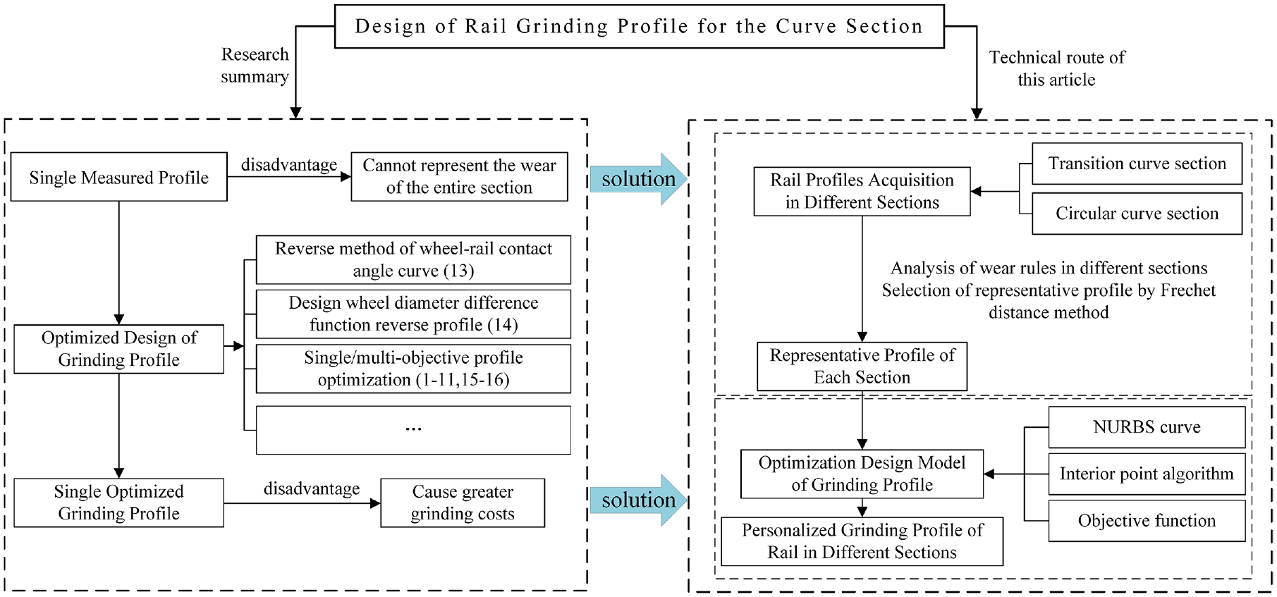
Research summary and the technical route of this paper.

Selection of Representative Profiles

Collection of the Rail Wear Data

The rail profile of the grinding section of the Daqin heavy-haul railway is collected. The grinding section is a curve section with a radius R of 800 m. The length of the transition curve is 100 m, and the length of the circular curve is 213 m. The wear profile is collected by a Miniprof measuring instrument with an interval of 20 m. Figure 2 shows the outer rail profiles measured in different sections.

Figure 2.

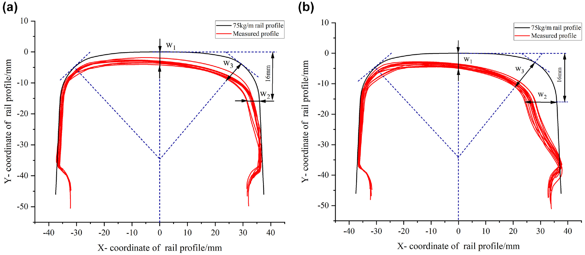
Outer rail profiles in the curve section: (a) transition curve section and (b) circular curve section.

According to the position and degree of wear in the curve section, the worn rails are described by three parameter indexes, namely $w_{1}$ (representing the rail wear depth downward from the centerline of the rail top), $w_{2}$ (representing the rail wear depth of the working side downward from the top of the rail at 16 mm), and $w_{3}$ (representing the rail wear depth in the normal direction of the wheel–rail contact point at the gauge corner).

According to the analysis in Figure 2, it can be seen that the wear in the circular curve section is larger than in the transition curve section. In the transition curve section, the wear is mainly concentrated at the rail top, $w_{1}$ reaches 4 mm, and the wear interval is mainly in [−25,30] mm. In the circular curve section, the wear is mainly concentrated at the gauge corner and inner side of the rail, $w_{2}$ and $w_{3}$ reach 11 mm, and the wear interval is mainly in [−25,35] mm. The main reason is that when the train passes through the curve, the wheelset will have a large lateral shift to improve the curve guiding ability of the train. The smaller the curve radius, the greater the lateral displacement, resulting in the wheel angle and the lateral force of the wheel–rail being greater, and the wear of the flange and the rail side being more serious.

Selection of Representative Profile Based on the Frechet Distance

In an actual railway line, because of the complex wheel–rail relationship, there are differences in the condition of rail wear at different locations. Therefore, the rail profiles in different parts of the transition curve section and circular curve section are compared, and the representative profiles that can represent the wear of different sections are selected as the initial conditions of profile design, which is crucial to the design results.

The Frechet distance is a method to solve the spatial path similarity, and it is used to judge the similarity of two curves. Assume that the binary group (S,d) is a metric space, where d is a metric function on S. For any two continuous curves A and B on S, there are A: [0,1]→S, B:[0,1]→S, and for two parameterized functions $α$ and $β$ on the unit interval, there are $α$ : [0,1]→S, $β$ : [0,1]→S, $α (0) = 0$ , $α (1) = N$ , $β (0) = 0$ , $β (1) = N$ ( 12 ).

Then the Frechet distance of curves A and B is as follows:

F (A, B) = min_{\binom{α [0, 1] \to [0, M]}{β [0, 1] \to [0, N]}} = {max d [A (α (T)), B (β (T))]}

(1)

In this paper, the representative worn rail profile is selected as the input condition of grinding profile design by using the Frechet distance method. Figure 3 is the schematic diagram of solving the representative profile by the Frechet distance method.

Figure 3.

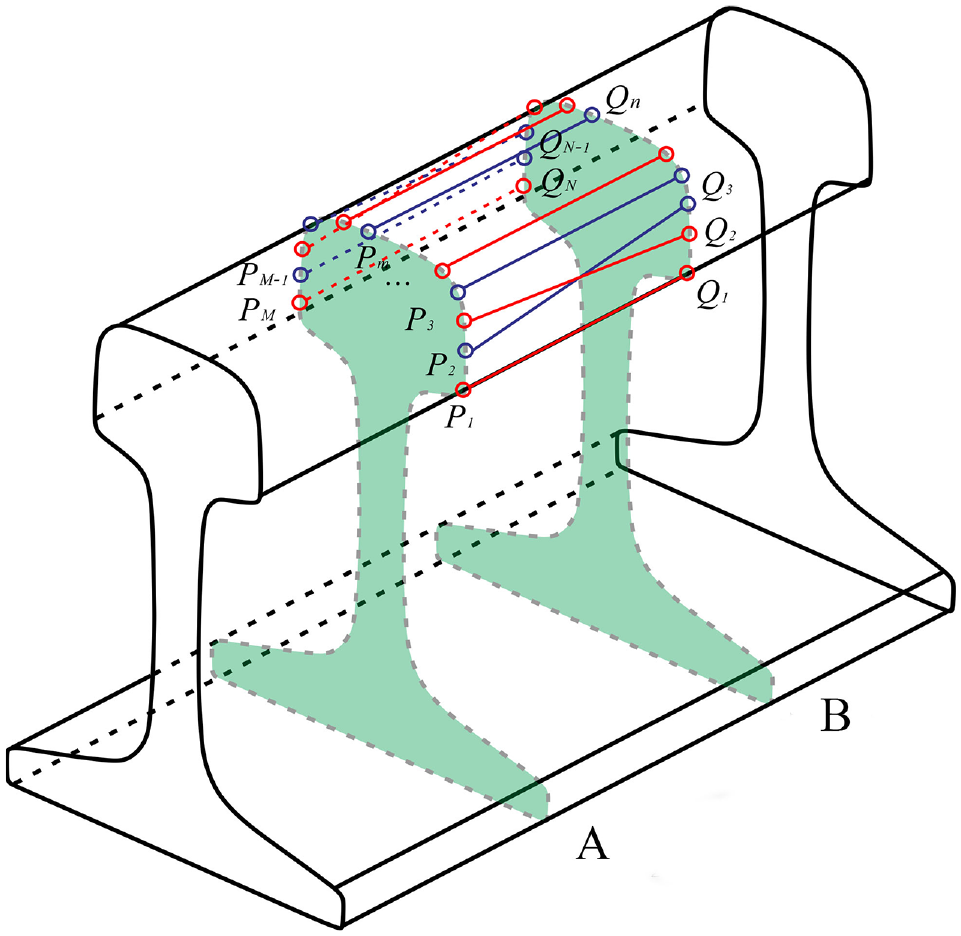
The Frechet distance method for a representative rail profile.

(1) For measured profiles of the worn rail in the curve section, any two worn rail profiles are taken as rail sections A and B, respectively. By calculating the distance $d_{mn}$ between each discrete point on sections A and B, matrix $D$ can be obtained:

D = (\begin{matrix} d_{11} & \dots & d_{1 n} & \dots & d_{1 N} \\ ⋮ & ⋮ & ⋮ \\ d_{m 1} & \dots & d_{mn} & \dots & d_{mN} \\ ⋮ & ⋮ & ⋮ \\ d_{M 1} & \dots & d_{Mn} & \dots & d_{MN} \end{matrix})

(2)

(2) Output the maximum $d_{max}$ and minimum distances $d_{min}$ in the matrix $D$ , initial target distance $f = d_{min}$ , and set the distance increment $ε$ :

ε = \frac{d_{max} - d_{min}}{100}

(3)

(3) The value greater than $f$ in the distance matrix $D$ is set to 0, and the value less than or equal to $f$ is set to 1. The binary matrix $D'$ is obtained by binary processing. A path $R$ with starting point $d'_{11}$ and ending point $d'_{MN}$ is searched in the binary matrix $D'$ . When the path $R$ passes through the path point $d'_{mn}$ , the next path point can only be selected from the path points $d'_{(m + 1) n}$ , $d'_{m (n + 1)}$ , and $d'_{(m + 1) (n + 1)}$ . All points in the path $R$ must be 1. At this time, there is a path $R$ :

{\begin{matrix} R = {d'_{11}, \dots, d'_{mn}, \dots, d'_{MN}} \\ d'_{11} = \dots = d'_{mn} = d'_{(m + k) (m + k')} = \dots = d'_{(MN)} = 1 \end{matrix}

(4)

where $1 \leq m + k \leq M, 1 \leq n + k' \leq M, k = {0, 1}, k' = {0, 1}$ .

(4) If path $R$ exists or $f = d_{max}$ , the Frechet distance between the two worn rail profiles is $F = f$ ; if path $R$ does not exist, then the target distance is set to $f = f + ε$ ; repeat step (3) until path $R$ is found.

(5) The Frechet distance $F = f_{ik}$ between two arbitrary worn rail profiles $i$ and $k$ can be calculated. Then the Frechet distance between the $i$ profile and the residual profiles can be defined by the following equation:

F_{i} = f_{sum} = \sum_{k = 1}^{Z} f_{ik}

(5)

where $i$ and $k$ represent the number of measured rail profiles; $Z$ represents the total number of measured rail profiles.

Based on the measured 10 profiles in the transition curve and circular curve sections, respectively, and according to the above Frechet distance method, the Frechet distances of the rail profiles in the transition curve section and the circular curve section are calculated; the obtained Frechet distances $F_{trans}$ and $F_{cons}$ are as follows:

{\begin{matrix} F_{trans} = {\begin{matrix} 41.13, 37.93, 39.95, 53.19, 49.23, 39.74, \\ 39.50, 37.77, 50.16, 39.02 \end{matrix}} \\ F_{cons} = {\begin{matrix} 39.19, 35.05, 34.78, 37.14, 59.09, 35.61, \\ 46.77, 48.92, 59.33, 27.47 \end{matrix}} \end{matrix}

(6)

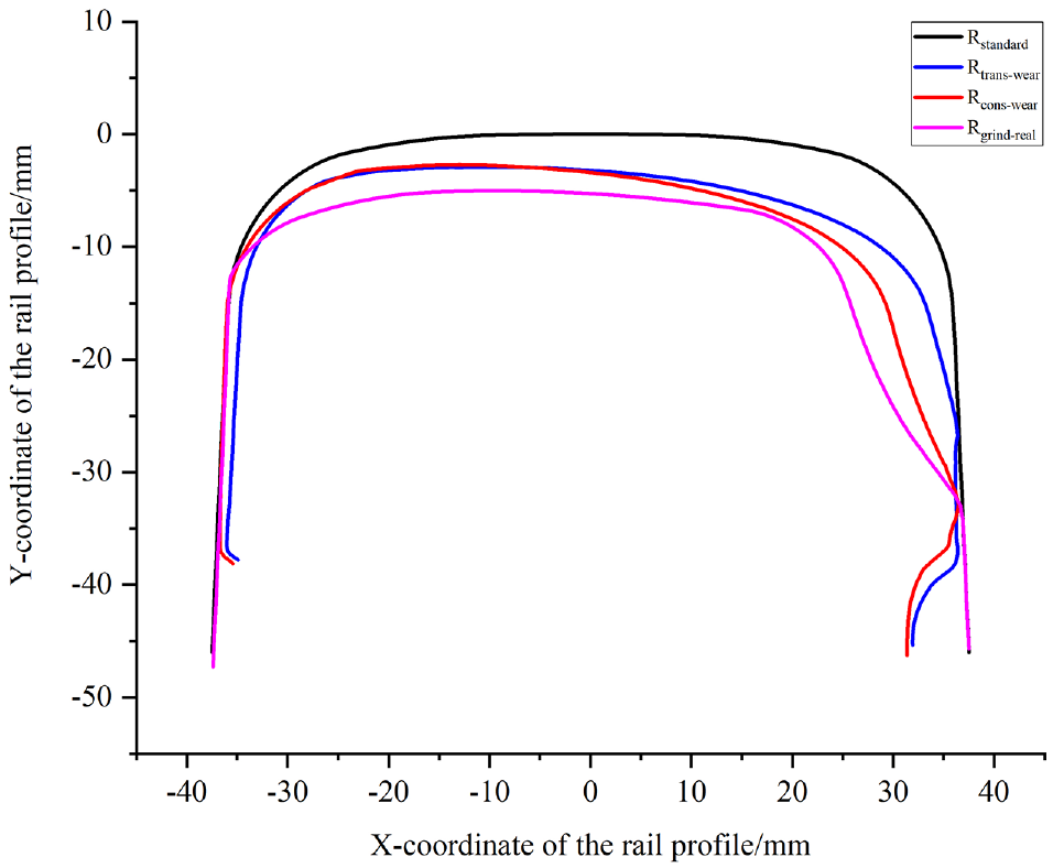
It can be known from the calculation results that the minimum Frechet distances in the transition curve section and the circular curve section are 37.77 and 27.47, respectively. The representative profile $R_{trans - wear}$ of the transition curve section and the representative profile $R_{cons - wear}$ of the circular curve section are shown in Figure 4, where $R_{grind - real}$ is the measured grinding profile in the field.

Figure 4.

Representative profiles.

Design of a Rail Profile Based on the Non-Uniform Rational B-Spline Curve

Definition and Geometric Characteristics of the NURBS Curve

A k-order NURBS curve can be defined as a piecewise rational polynomial vector function:

p (u) = \frac{\sum_{i = 0}^{n} ω_{i} d_{i} N_{i, k} (u)}{\sum_{i = 0}^{n} ω_{i} N_{i, k} (u)} (0 \leq u \leq 1)

(7)

where $ω_{i} (i = 0, 1, \dots, n)$ is called weight factor; $d_{i} (i = 0, 1, \dots, n)$ is the control point; and $N_{i, k} (u)$ is called the k-order canonical B-spline basis function, which is calculated by the node vector through the Cox–de Boor algorithm ( 18 ).

In the optimization design of the rail profile, the NURBS mainly has the following geometric characteristics.

(1) Local modification

The NURBS curve has the characteristics of local modification. In the iterative process of rail profile optimization in different sections, the position and weight factors of local finite control points of the NURBS curve can be adjusted to realize local modification of the curve shape, so as to obtain a new reconstructed profile.

(2) Geometric continuity

By modifying the weight factor, the local shape curve of the rail profile can be changed, but it will not affect the smoothness of the connection of other sections. The rail optimization based on the NURBS curve can ensure the smoothness and continuity of the profile curve.

(3) Strong convex hull

In the process of rail profile design, to obtain better wheel–rail contact, there is no two-point contact in the contact process. It is necessary to acquire the anti-conformal contact between the wheel tread and the rail top, and the conformal contact between the rail gauge angle and the wheel flange. The geometric characteristics of the rail determine that the rail curve is a strictly convex function, so the convexity of the NURBS provides a convenient condition for the design of the rail profile.

Optimal Control Point Solution Based on the Interior Point Algorithm

To obtain profiles of the rail grinding target, the rail curve is first treated as a parameterized discrete point, and a limited number of discrete points are selected as the initial control points, which are used as the design variables of the rail NURBS curve fitting. The interior point algorithm is used to obtain the optimal control point of the NURBS curve. By setting the optimization objective function and the feasible region interval, a new penalty function is constructed, and the constrained optimization problem is transformed into a new unconstrained optimization problem. Therefore, the output solution is guaranteed to be feasible. Through continuous optimization iteration in the feasible region, the penalty function converges and the extreme point is obtained.

The objective function of the interior point algorithm can be defined as follows:

min f (x), x \in R^{n}

(8)

g_{i} (x) \leq 0 (i = 1, 2, \dots, m)

(9)

In the optimization iterative solution, the constructed penalty function can be defined as follows:

ξ (X, r) = f (X) - r \sum_{i = 1}^{m} \frac{1}{g_{i} (X)}

(10)

where $r$ is a penalty factor, which is a sequence of positive numbers decreasing in turn, satisfying $lim_{k \to \infty} r = 0$ .

When the NURBS curve is used to solve the optimal control point, the objective function is to reduce rail grinding amount, which can be defined as follows:

S {(x)}_{min} = \int_{a}^{b} f_{R_{origin}} (x) dx - \int_{a}^{b} f_{R_{reconstruct}} (x) dx

(11)

G {(x)}_{min} = g_{i, origin} (x) - g_{i, reconstruct} (x) \leq 0

(12)

where $\int_{a}^{b} f_{R_{origin}} (x) dx$ and $\int_{a}^{b} f_{R_{reconstru ct}} (x) dx$ represent the area enclosed by the initial rail profile and the reconstructed profile in the feasible region $[a, b] \in [- 35.5, 36.5]$ and the straight line $y = 0$ , respectively. The design requires $S {(x)}_{min}$ to be as small as possible, that is, the rail grinding amount is the minimum; $g_{i, origin} (x)$ and $g_{i, reconstruct} (x)$ represents the ordinate values corresponding to the $i$ th control point $d_{i}$ in the feasible region, respectively. The design requires $G {(x)}_{min}$ to be as small as possible to ensure the fitting accuracy.

The feasible region for optimization can be defined as follows:

{\begin{matrix} x \in [- 36.0, 36.0] \\ y \in [- 12, 0] \end{matrix}

(13)

{\begin{matrix} f'_{R_{origin}} \leq 0 \\ f ″_{R_{reconstruct}} \leq 0 \end{matrix}

(14)

The penalty function constructed can be defined as follows:

ξ (X, r) = S (X) - r \sum_{i = 1}^{i} \frac{1}{g_{i} (X)}

(15)

The extreme value condition is used to solve the solution of Equation 15, and the extreme point of the penalty function is obtained.

Establishment of the Optimization Design Model

Objective Functions

(1) Objective function for reducing grinding removal of rail materials

f_{1, min} = S {(x)}_{min} = \int_{a}^{b} f_{R_{origin}} (x) dx - \int_{a}^{b} f_{R_{reconstruct}} (x) dx

(16)

Each symbol in the equation represents the same meaning as Equation 11.

(2) Objective function for improving wheel–rail contact geometry

The rail curve is discretized, and the track method ( 19 ) is used to solve the wheel–rail contact points in the optimization iteration process of the cubic NURBS curve. The principle of optimal design should ensure that the wheel–rail contact geometry of the profile reconstructed by the NURBS curve is infinitely close to the wheel–rail contact geometry of a standard 75 kg/m rail, and ensure that the wheel–rail contact uniformity is significantly improved.

In the process of solving the geometric relationship of wheel–rail contact, taking the left-hand wheel–rail contact as an example, the coordinates of the wheel–rail contact points can be defined by the following ( 20 ):

{\begin{matrix} x_{c} = - \cos θ \sin φ (η_{L} - R_{L} \tan δ_{L}) \\ y_{c} = a \cos θ \cos φ + b \sin θ \\ z_{c} = - a \sin θ + b \cos θ cons φ \end{matrix}

(17)

where a and b can be defined as follows:

{\begin{matrix} a = η_{L} + R_{L} \tan δ_{L} \cos^{2} θ \sin^{2} φ / (\cos^{2} θ \cos^{2} φ + \sin^{2} θ) \\ b = R_{L} \sqrt{\cos^{2} θ \cos^{2} φ + \sin^{2} θ - \cos^{2} θ \sin^{2} φ \tan^{2} δ_{L}} / (\cos^{2} θ \cos^{2} φ + \sin^{2} θ) \end{matrix}

(18)

where $θ$ is the correction angle of the wheel–rail roll angle; $φ$ is the yaw angle; $η_{L}$ is the lateral distance from the wheelset centroid to the discrete point of the left-hand wheel tread; $δ_{L}$ is the wheel–rail contact angle of the left-hand wheel; and $R_{L}$ is the rolling circle radius of the wheel.

After calculating the coordinates of the contact points between the wheel and rail, the difference between the horizontal coordinates $x_{c 1}$ and $x_{cn}$ of the two farthest contact points on the rail is calculated and used as the contact interval $L_{contact}$ , which can be defined as follows:

L_{contact} = x_{ci} - x_{c 1} (i \in [1, n])

(19)

All the contact points in the interval are projected onto the interval. The contact tolerance $τ$ is set, and $τ = 1 mm$ is taken. The effective contact length $l_{c}$ of all the contact points in the interval is counted, and the wheel–rail point density $ρ_{c}$ is calculated.

The difference between the horizontal coordinates of two adjacent contact points shall satisfy the following:

l_{cn} = x_{i + 1} - x_{i} < τ (i \in [1, n])

(20)

The density of the wheel–rail contact point $ρ_{c}$ can be defined as follows:

ρ_{c} = \frac{l_{c 1} + l_{c 2} + \dots + l_{ci}}{x_{ci} - x_{c 1}} = \frac{\sum_{i = 1}^{n} l_{ci}}{L_{contact}} (i \in [1, n])

(21)

Therefore, the objective function of improving the wheel–rail contact geometry is as follows:

f_{2, min} = \frac{1}{ρ_{c_reconstruct}}

(22)

where $ρ_{c_reconstruct}$ represents the density of wheel–rail contact points of the rail grinding profile reconstructed by the NURBS curve.

The wheel–rail contact geometry reconstructed by the NURBS curve should satisfy the following:

ρ_{c_wear} < ρ_{c_reconstruct}

(23)

where $ρ_{c_wear}$ represents the density of the wheel–rail contact points of the initial worn rail profile.

(3) Comprehensive optimization objective function

Taking into account the difference in the magnitude of the two objective functions, the normalization is used, and the weighted sum of the two objectives is used as the comprehensive objective function. The comprehensive objective function $f (T)$ is as follows:

f (T) = ω_{1} \bar{f_{1, min}} + ω_{2} \bar{f_{2, min}}

(24)

where $ω_{1}$ and $ω_{2}$ are the weight of the rail grinding amount and the density of the wheel–rail contact points, respectively, $ω_{1} = ω_{2} = 0.5$ in this paper. Here, $\bar{f_{1, min}}$ is the normalized index of the rail grinding amount; $\bar{f_{2, min}}$ is the normalized index of the density of the wheel–rail contact points.

Constraint Functions

(1) Constraints on upper and lower boundaries

When the center point of the rail top surface reaches the critical vertical grinding amount of 12 mm downward, it is a serious rail, and the rail should be replaced in time ( 21 ). When designing the rail profile, the center point of the rail top surface is defined as the design origin, and constraints on the left- and right-hand boundaries of the rail profile are defined as follows:

f_{R_{reconstruct | x = 0}} (x) \in [- 12, 0]

(25)

where $f_{R_{reconstruct}} (x)$ represents the function value at x = 0 after reconstructing the rail profile by the NURBS curve.

(2) Constraints on the left- and right-hand boundaries

Since the rail wear is mainly concentrated in the railhead area, at the same time, to reduce the number of control points and improve the computational efficiency, the left- and right-hand boundary constraints of the optimized profile are defined:

x_{R_{reconstruct}} \in [- 35.5, 36.5]

(26)

where $x_{R_{reconstruct}}$ represents the horizontal coordinate value of the control points when the profile is designed by the NURBS curve.

(3) Concave–convex constraint

According to the description of the rail profile, the curve section of the main contact part between the wheel and rail should be set as a convex curve, and the concave–convex constraint of the rail optimized profile is defined as follows:

f ″_{R_{reconstruct}} (x) < 0

(27)

Optimization Process

The discrete points of the worn rail profile are taken as input, and the LM worn wheel tread is selected as the wheel profile. The comprehensive optimization objective function and constraint function are input. Based on the interior point algorithm, the optimal control point of the NURBS curve is solved. The current control point is adjusted and iteratively optimized by the fmincon optimization function. The NURBS curve fitting of the profile is carried out by cubic NURBS curve theory to obtain a new rail profile. The wheel–rail contact geometric relationship and grinding amount of the optimized profile are solved to determine whether the optimization goal is met. If the goal is met, the optimization solution is output. If it is not satisfied, the number of iterations is specified to recalculate. The optimization process is shown in Figure 5. The optimal solution is obtained by trial calculation of multiple specified iterations of the objective function value.

Figure 5.

The optimization process of the grinding profile.

Case Analysis

According to the wear law of the transition curve section and the circular curve section, the worn rail profile is reconstructed by the NURBS curve. In this paper, 18 control points are selected for cubic NURBS curve fitting. The current control point is used as the initial control point, and the optimization iteration is carried out along the descending direction of the objective function. The function convergence obtains the optimal solution. 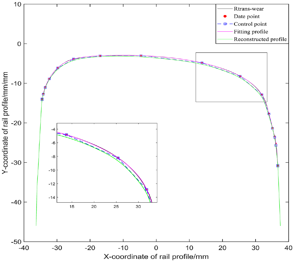Optimized design profiles $R_{trans - opt}$ for the transition section and $R_{cons - opt}$ for the circular curve section are obtained. Table 1 shows the main design parameters of the transition curve section using the cubic NURBS curve, and Figure 6 shows the grinding profile designed for the transition curve section by the cubic NURBS curve.

Figure 6.

Optimized design grinding profile in the transition curve section.

Table 1.

Parameters for Cubic Non-Uniform Rational B-Spline Design in the Transition Curve Section

Initial data point $d_{i}$			Weight factor ω_i		Optimal control point $d'_{i}$
i	x_i	y_i	i	ω_i	i	x_i	y_i
0	na	na	0	1	0	−35.49	−14.13
1	−34.48	−13.93	1	1	1	−34.48	−13.93
2	−34.12	−12.63	2	0.15	2	−34.12	−12.73
3	−33.54	−10.96	3	0.94	3	−33.54	−11.07
4	−31.65	−8.87	4	0.94	4	−31.65	−8.89
5	−28.70	−6.09	5	0.88	5	−28.70	−6.14
6	−24.25	−3.87	6	0.64	6	−24.25	−3.88
7	−17.55	−3.05	7	0.37	7	−17.55	−3.03
8	−7.55	−3.02	8	0.44	8	−7.55	−4.83
9	7.55	−4.83	9	0.87	9	7.55	−8.23
10	17.55	−8.22	10	0.91	10	17.55	−12.87
11	24.25	−12.85	11	0.39	11	24.25	−17.74
12	28.70	−17.64	12	0.07	12	28.70	−21.74
13	31.65	−21.31	13	0.09	13	31.65	−21.39
14	33.65	−23.36	14	0.43	14	33.65	−23.61
15	34.95	−25.19	15	0.63	15	34.95	−25.67
16	35.94	−30.71	16	1	16	35.94	−30.71
17	na	na	17	1	17	35.49	−30.91

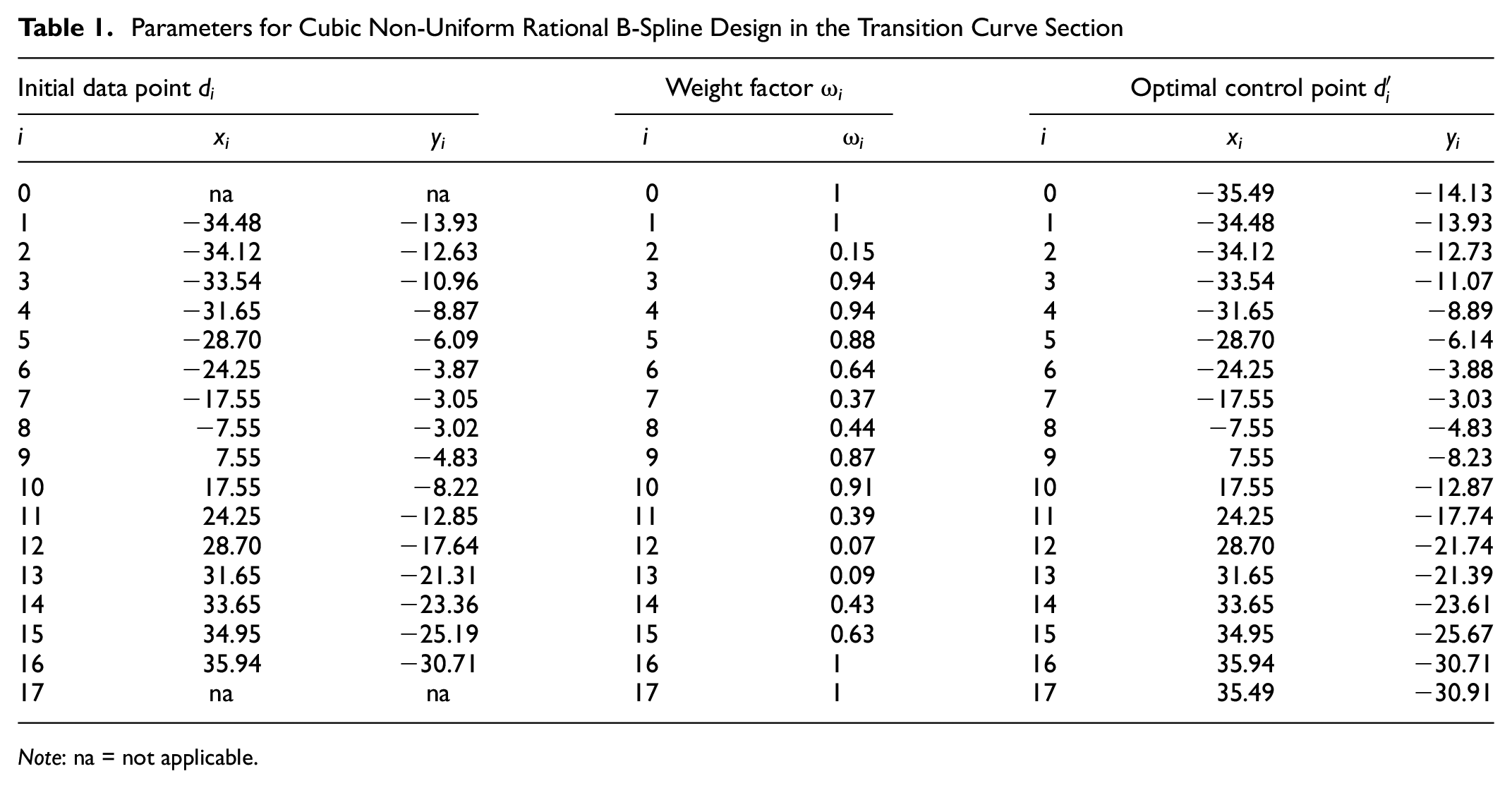
Note: na = not applicable.

Table 2 shows the main design parameters of the circular curve section using the cubic NURBS curve, and Figure 7 shows the grinding profile designed for the circular curve section by the cubic NURBS curve.

Figure 7.

Optimized design grinding profile in the circular curve section.

Table 2.

Parameters for Cubic Non-Uniform Rational B-Spline Design in the Circular Curve Section

Initial data point $d_{i}$			Weight factor ω_i		Optimal control point $d'_{i}$
i	x_i	y_i	i	ω_i	i	x_i	y_i
0	na	na	0	1	0	−35.49	−10.76
1	−34.48	−10.56	1	1	1	−34.48	−10.56
2	−33.65	−9.44	2	0.36	2	−33.65	−9.64
3	−32.51	−8.11	3	0.63	3	−32.51	−8.32
4	−30.77	−6.59	4	0.91	4	−30.77	−6.78
5	−27.48	−4.76	5	0.63	5	−27.48	−4.94
6	−22.35	−3.22	6	0.53	6	−22.35	−4.32
7	−13.99	−2.71	7	0.16	7	−13.99	−4.00
8	−2.36	−3.17	8	0.26	8	−2.36	−4.24
9	16.05	−6.22	9	0.95	9	16.05	−5.78
10	26.67	−11.47	10	0.99	10	26.67	−11.58
11	30.46	−18.60	11	0.39	11	30.46	−18.82
12	32.32	−23.51	12	0.19	12	32.32	−24.81
13	33.91	−27.07	13	0.30	13	33.91	−27.50
14	34.97	−29.12	14	0.62	14	34.97	−29.51
15	35.86	−31.07	15	0.28	15	35.86	−31.28
16	36.46	−32.67	16	1	16	36.46	−32.67
17	na	na	17	1	17	36.47	−32.87

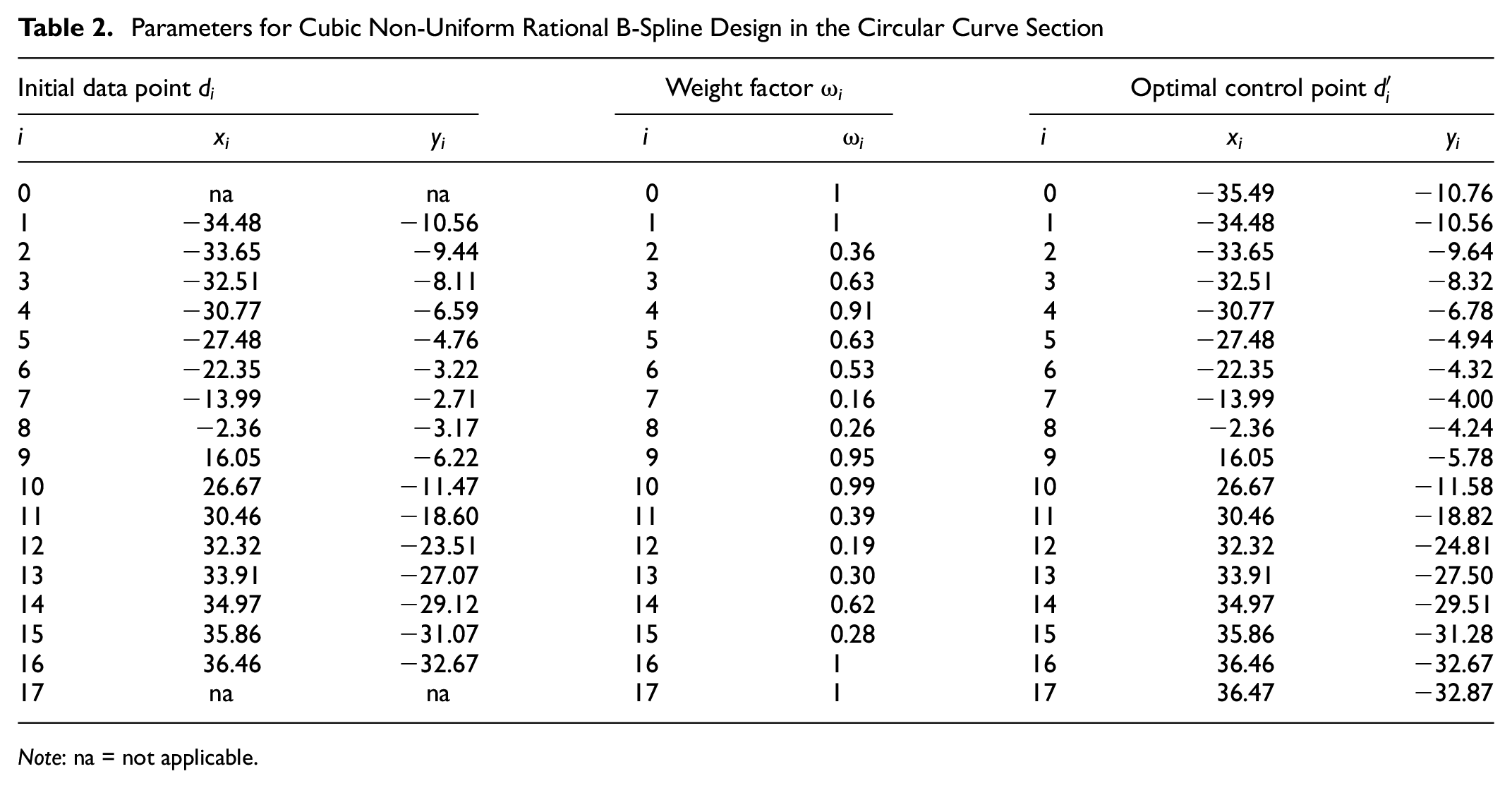
Note: na = not applicable.

The wheel–rail contact geometry directly reflects the area of wheel–rail contact frequently. Figure 8 shows the wheel–rail contact geometry of the representative profiles, optimized profiles, and measured grinding profile matched with the LM wheel. Through comparative analysis, it is known that the state of the wheel–rail contact points of the measured grinding profile is better than the representative profile. However, the contact points still have jumps, which will lead to uneven wear. The range of wheel–rail contact points with the optimized profile is obviously expanded and distributed more evenly without the jumping phenomenon, which is beneficial to make the force of the railhead more uniform and reduce the local wear of the railhead.

Figure 8.

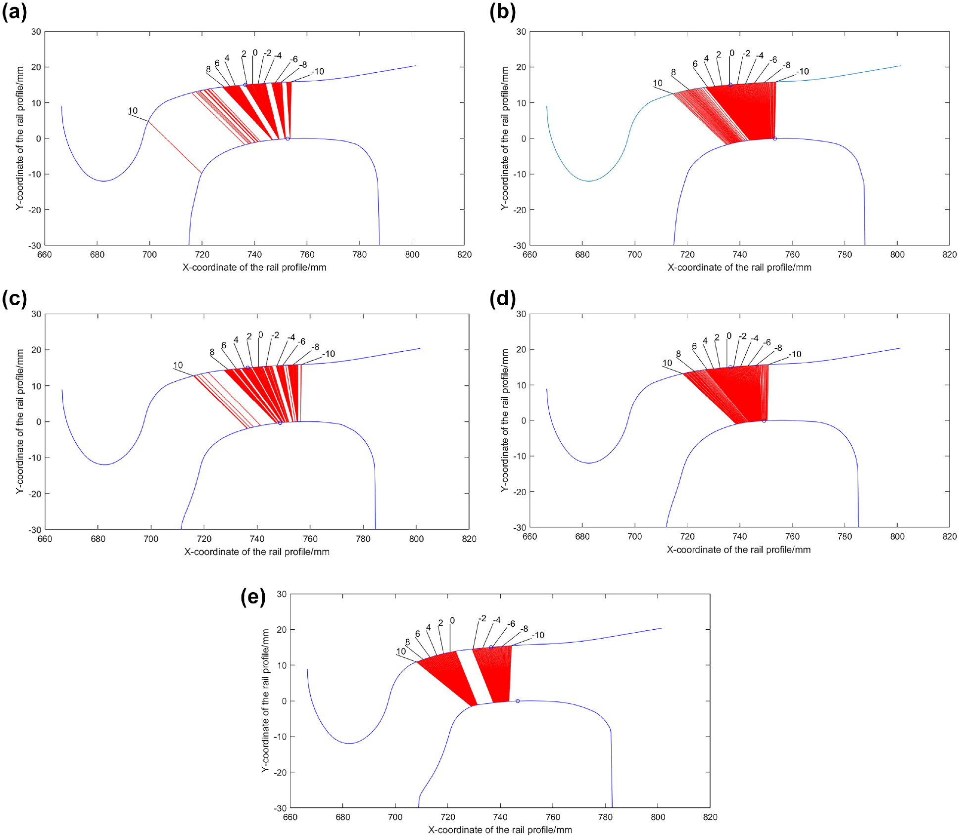
Wheel–rail contact geometry: (a) $R_{trans - wear}$ , (b) $R_{trans - opt}$ , (c) $R_{cons - wear}$ , (d) $R_{cons - opt}$ , and (e) $R_{grind - real}$ .

As shown in Figure 6, in the optimization iteration process of the cubic NURBS curve, the geometric continuity and strong convex hull of the NURBS curve ensure the smoothness of the reconstructed curve. As a grinding profile, it can avoid the two-point contact in the geometric relationship of wheel–rail contact and significantly reduce the contact stress between the wheel and rail. It can be seen from Table 3 that the grinding amount of $R_{trans - opt}$ is 32.62 mm², which is reduced by 80.1% compared with 163.87 mm² of $R_{grind - real}$ . The wheel–rail contact density of $R_{trans - opt}$ is 94.71%. Compared with 9.77% of $R_{trans - wear}$ , the wheel–rail contact uniformity has been significantly improved, increasing by 869.4%, which can effectively improve the stress concentration in the wheel–rail contact process and prolong the service life of the rail.

Table 3.

Parameter Indexes for Optimized Profiles in the Curve Section

Rail profile	Accuracy of fitting	Grinding amount (mm²)	Contact length (mm)	Effective wheel–rail contact length (mm)	Wheel–rail contact density (%)
$R_{trans - opt}$	0.0302	32.62	18.90	17.90	94.71
$R_{cons - opt}$	0.0284	145.43	7.30	7.30	100.00
$R_{trans - wear}$	na	na	39.90	3.90	9.77
$R_{cons - wear}$	na	na	20.10	6.40	31.80
$R_{grind - real}$	na	163.87	14.40	8.30	57.64

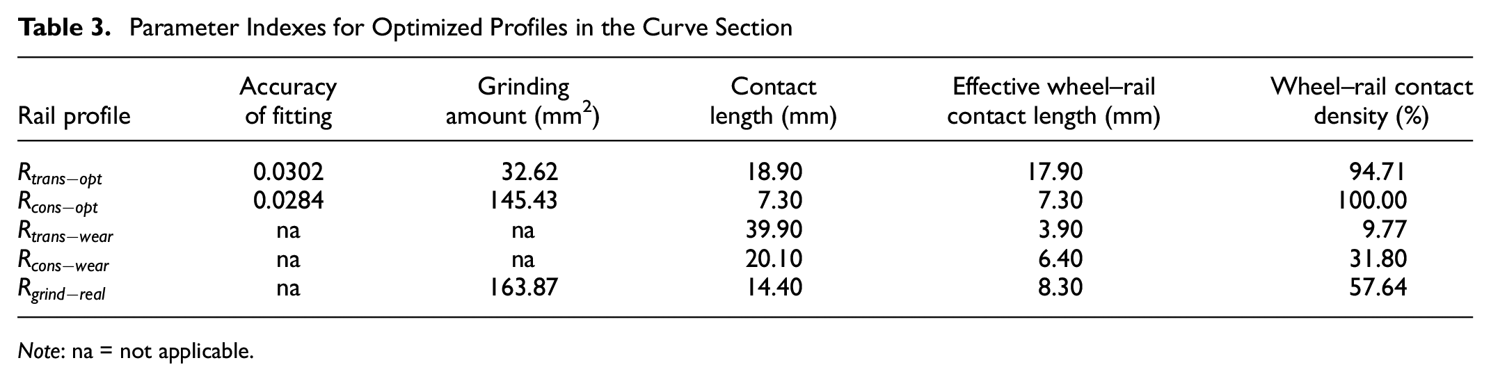
Note: na = not applicable.

As shown in Figure 7, the wear at the gauge corner in the circular curve section is obvious. In the optimization iteration process of the cubic NURBS curve, by adjusting the position and weight factor of the control point at the gauge corner, the contact position between the gauge corner and the wheel flange is improved, and the geometric distribution of the wheel–rail contact at the gauge corner is more uniform, which reduces the contact stress between the wheel and rail. It can be seen from Table 3 that the grinding material removed of the optimized design profile $R_{cons - opt}$ in the circular curve section is 145.43 mm², which is 11.3% less compared to $R_{grind - real}$ . The wheel–rail contact density of $R_{cons - opt}$ is 100%. Compared with the 31.84% of $R_{cons - wear}$ , the wheel–rail contact uniformity is improved by 214.1%, which slows down the serious rail eccentric wear caused by the concentrated contact between the wheel flange and rail distance angle when the train passes the curve and extends the service life of the rail.

Wheel–Rail Dynamics and Finite Element Analysis

Dynamics Analysis

Evaluation Index of Dynamic Performance

The dynamic model of the Chinese heavy-haul freight train C96 was established, as shown in Figure 9. Referring to the measured line, the line condition of the model is set as the total length of the track, which is 500 m, and the length of the front and back straight lines is 50 m, respectively. The length of the inlet and outlet transition curve section are set to 100 m, respectively. The bottom slope of the track is set to 1/40 and the wheel profile is LM.

Figure 9.

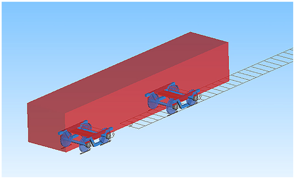
C96 dynamic model of a heavy-haul freight train.

The derailment coefficient, rate of wheel load reduction, wheelset lateral force, and lateral vibration acceleration of the carbody are used to evaluate the dynamic performance ( 22 ). By comparing the dynamic operation characteristics of the measured grinding profile ( $R_{grind - real}$ ) and optimized grinding profiles ( $R_{opt}$ ) at different running velocities and different curve radii, the adaptability of the optimized grinding profile was analyzed.

(1) Derailment coefficient

The derailment coefficient is used to evaluate whether the wheel flange will climb the rail head and derail under the action of lateral force. It is the ratio of lateral force to vertical force of the wheel acting on the rail, that is, the derailment coefficient is $\frac{Q}{P}$ . For freight trains, the safety limit of the derailment coefficient is $\frac{Q}{P} \leq 1.0$ when the curve radius $R \geq 400 m$ .

(2) Rate of wheel load reduction

The rate of wheel load reduction is another safety index for evaluating derailment caused by excessive wheel load reduction, which is the ratio of the wheel load reduction amount to the average static wheel load of the shaft, namely, the rate of wheel load reduction is $\frac{Δ P}{\bar{P}}$ . Here, $\frac{Δ P}{\bar{P}} \leq 0.65$ when the velocity $v \leq 160 km / h$ .

(3) Wheelset lateral force

The wheelset lateral force H is used to evaluate whether the vehicle will cause the gauge to widen or serious deformation of the line because of excessive lateral force during operation. The limit value of H is as follows:

H \leq 15 + \frac{P_{0}}{3}

(28)

where $P_{0}$ is the static axle load (kN).

(4) Lateral vibration acceleration of the carbody

Lateral vibration acceleration of the carbody $a_{ty}$ is used to evaluate the running quality of the vehicle. For freight trains, $a_{ty} \leq 3 m / s^{2}$ .

Adaptability Analysis of Running Velocity

When the vehicle runs at different velocities, it will have a certain impact on the force between the wheel and rail. Therefore, this paper studies the dynamic response when the curve radius R is 800 m and the vehicle velocity is 60–100 km/h, as shown in Figure 10. It can be seen from Figure 10, a and b , that when the velocity is in the range of 60–100 km/h, the derailment coefficient and rate of wheel load reduction of $R_{grind - real}$ and $R_{opt}$ increase with the increase of velocity. Under different operating velocities, the derailment coefficient and wheel load reduction rate of $R_{opt}$ decrease significantly, and the average decrease of the derailment coefficient and rate of wheel load reduction rate reach 10.15% and 13.69%, respectively. It can be seen from Figure 10c that on the whole, the H values of $R_{grind - real}$ and $R_{opt}$ show an upward trend, and the H value of $R_{opt}$ is lower than that of $R_{grind - real}$ , with an average decrease of 11.78%. Figure 10d shows that the $a_{ty}$ values of $R_{grind - real}$ _l and R_opt increase linearly with velocity and are lower than the safety limit. At different velocities, the $a_{ty}$ value of R_opt is lower than that of $R_{grind - real}$ , and the average reduction of $a_{ty}$ is 20.13%.

Figure 10.

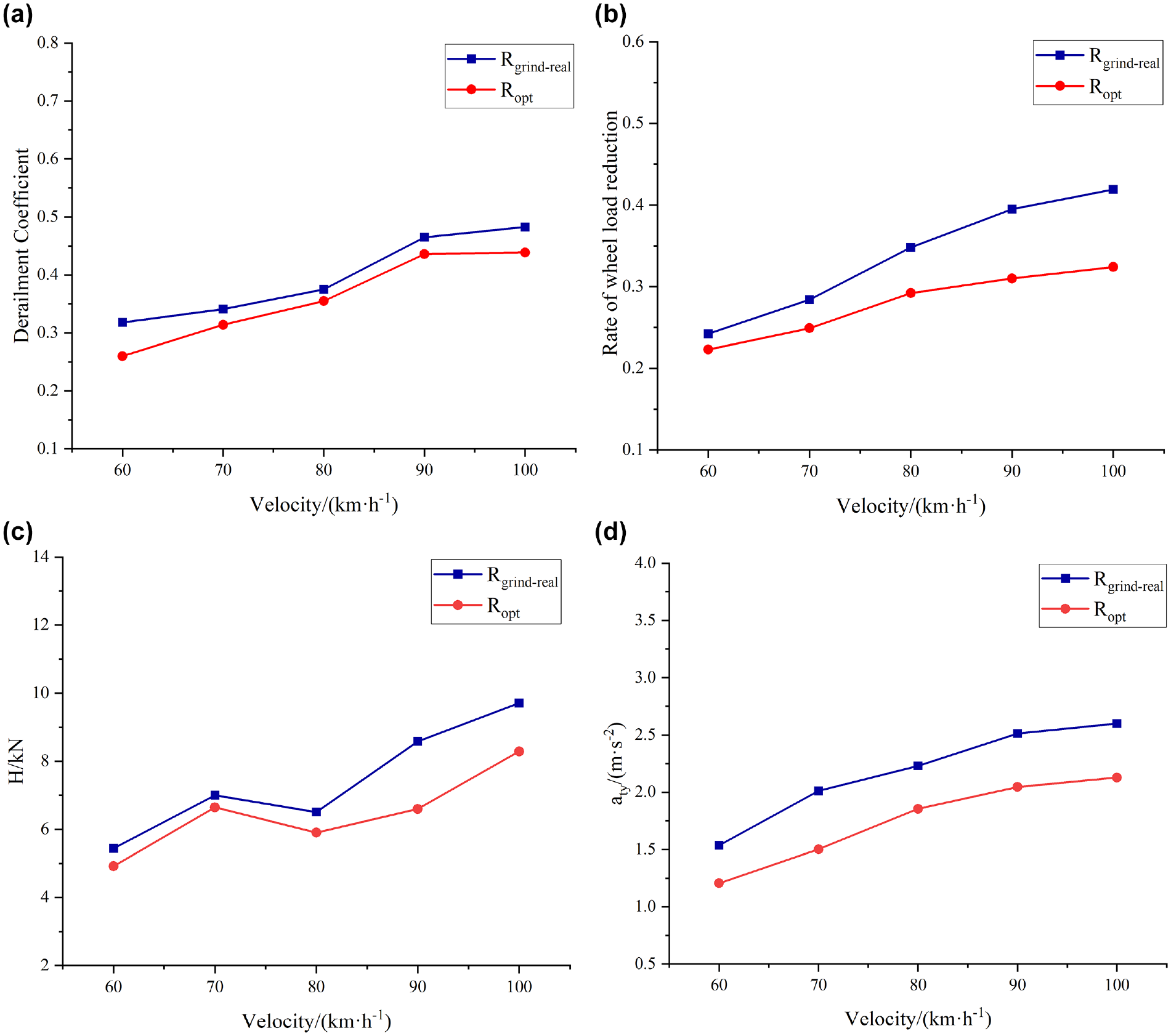
Comparison of dynamic characteristics under different running velocities: (a) derailment coefficient, (b) rate of wheel load reduction, (c) wheelset lateral force, and (d) lateral vibration acceleration of the carbody.

The above are the dynamic characteristics of the measured grinding profile and the optimized grinding profile under different vehicle velocities. In the velocity range studied, the curve passing performance of the optimized grinding profile is improved compared with the measured grinding profile.

Adaptability Analysis of the Curve Radius

The curve radius has a significant influence on the dynamic performance. Therefore, the dynamic response is studied when the running velocity is 80 km/h and the curve radius is 400, 600, 800, 1000, and 1200 m, respectively, as shown in Figure 11. It can be seen from Figure 11a that with the increase of curve radius, the variation trend of the derailment coefficient of $R_{grind - real}$ and $R_{opt}$ is basically the same. When the curve radius is greater than 1000 m, the derailment coefficient tends to be stable. Under different curve radii, the derailment coefficient of $R_{opt}$ is significantly lower than that of $R_{grind - real}$ , with an average decrease of 7.47%. Figure 11, b and c , shows that the rate of wheel load reduction and H values of $R_{grind - real}$ and $R_{opt}$ decrease linearly with the increase of the curve radius. The rate of wheel load reduction and H values of $R_{opt}$ are significantly less than those of $R_{grind - real}$ , with an average decrease of 12.79% and 10.6%, respectively. It can be seen from Figure 11d that the $a_{ty}$ value of $R_{opt}$ is significantly reduced under different curve radii, with an average reduction of 21.51%.

Figure 11.

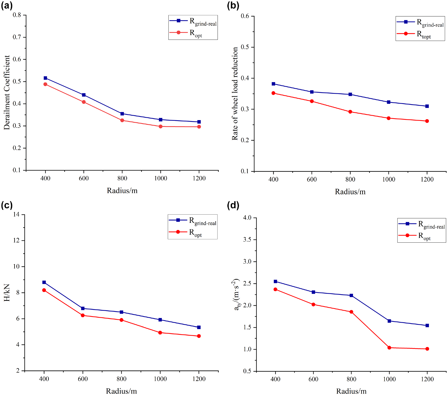
Comparison of dynamic characteristics under different different curve radii: (a) derailment coefficient, (b) rate of wheel load reduction, (c) wheelset lateral force, and (d) lateral vibration acceleration of the carbody.

The above are the dynamic characteristics of the measured grinding profile and optimized grinding profile under different curve radii. In the range of the studied curve radius, the dynamic evaluation index of the optimized grinding profile is significantly reduced, and the curve passing performance is significantly improved.

Equivalent Conicity Analysis

In the design of wheel–rail shape matching, the curve formed by the equivalent conicity value of the wheelset with different lateral displacements is called the “equivalent conicity curve” ( 23 ). As shown in Figure 12, on the whole, the equivalent conicity shows an upward trend, and the equivalent conicity of $R_{trans - opt}$ is less than that of $R_{grind - real}$ . When the wheelset lateral displacement is within [0,6] mm, the equivalent conicity is less than 0.08, which is a stable change. This trend is conducive to improving the operation performance of the straight line before and after the bending, and improving the critical speed of serpentine instability in the transition curve section. When the wheelset lateral displacement is within [6,10] mm, the equivalent taper of both showed a slow upward trend, which is conducive to the high-speed operation of the vehicle. The equivalent conicity of $R_{cons - opt}$ _t is greater than that of $R_{grind - real}$ and $R_{trans - opt}$ , and it shows an upward trend in the range of [1,10] mm, which is conducive to the automatic alignment of wheelsets and improves the curve passing performance of vehicles in the circular curve section.

Figure 12.

Comparison of the equivalent of conicity.

Finite Element Analysis of Wheel–Rail Contact

Considering the local plastic deformation of the wheel–rail contact area, the elastic–plastic contact model was adopted in this paper, and the yield condition was the von Mises yield criterion. The wheel–rail material adopts a bilinear elastic–plastic constitutive model, and the stress–strain equation is as follows:

σ = {\begin{matrix} E_{e} ε ε \leq ε_{s} \\ σ_{s} + E_{p} (ε - ε_{s}) ε > ε_{s} \end{matrix}

(29)

where $σ$ is stress; $ε$ is strain; $σ_{s}$ is the yield stress; $E_{e}$ is the Young’s modulus; $E_{p}$ is the strain hardening modulus; and $ε_{s}$ is the total strain at the yield point.

The rail material is U75V; the material parameters are shown in Table 4 and the stress–strain curve is shown in Figure 13. In addition, assume that the wheel material is the same as the rail ( 24 ).

Figure 13.

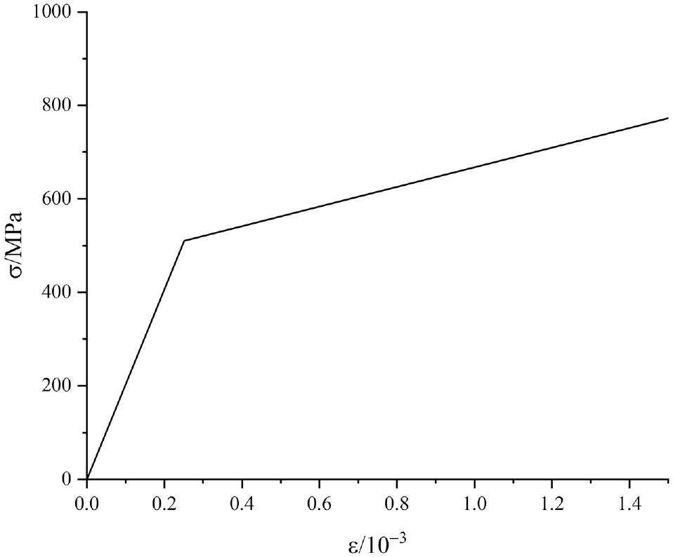
Stress–strain curve of the wheel–rail material.

Table 4.

Material Parameters of the Wheel and Rail

$σ_{s}$ /MPa	$E_{e}$ /GPa	$E_{p}$ /GPa	$ρ$ /(kg·m⁻³)	$ν$
510	203	21	7850	0.3

Rail profiles are optimized profiles and the measured grinding profile and the wheel profile are standard LM tread. Hypermesh is used for pre-processing of the model. The mesh size of the wheel–rail contact area is subdivided into 1 mm, and the mesh size of the non-contact area is gradually transitioned from 1 to 10 mm. All the meshes of the model adopt an eight-node linear hexahedron element. To simplify the calculation, the symmetry analysis is adopted, and a total of 182,182 mesh elements are divided. The model is imported into ABAQUS software and the static implicit algorithm is used to analyze the wheel–rail contact mechanical properties, as shown in Figure 14. In the calculation, the gauge is 1435 mm, the rail bottom slope is 1:40, the axle load is 25 t, and the wheelset has no yaw angle. In the boundary condition setting of wheel–rail contact, the rail bottom surface is set to be completely constrained. The axle is equivalent to a load node, and the axle load is applied to the node, which is point-to-surface coupled with the wheel diameter hole. The surface–surface contact is used for wheel–rail contact.

Figure 14.

Finite element model of wheel–rail contact: (a) mesh model of a single wheel and (b) mesh of the contact area.

It can be seen from the analysis in Figures 15 and 16a that when the wheelset lateral displacement is within [8,16] mm, the contact spot area of $R_{grind - real}$ shows a trend of sharp decrease and sharp increase. The contact spot area reaches the minimum value of 108.5 mm² when the wheelset lateral displacement is 16 mm, which is reduced by 41.3% compared with 184.9 mm² at 8 mm. This is because the wheel–rail contact presents a single point contact state on the flange, which leads to the reduction of the contact spot area. The change of the contact area of $R_{trans - opt}$ and $R_{cons - opt}$ is relatively flat. Here, $R_{grind - real}$ has two-point contact or conformal contact when the wheelset lateral displacement is within [12,20] mm, while for $R_{trans - opt}$ and $R_{cons - opt}$ two-point contact occurs at 20 mm, so the contact state of the optimized design profile is obviously improved.

Figure 15.

The change of contact spot with wheelset lateral displacement: (a) $R_{grind - real}$ , (b) $R_{trans - opt}$ , and (c) $R_{cons - opt}$ .

Figure 16.

Calculation of wheel–rail contact stress: (a) the change of contact spot area and (b) the change of maximum von Mises stress.

Figure 16b shows that the maximum von Mises stress of $R_{grind - real}$ has no obvious change when the wheelset lateral displacement is within [0,8] mm, but when the wheelset lateral displacement is within [8,16] mm, because of the stress concentration in advance, the stress of $R_{grind - real}$ increases significantly at 16 mm. The maximum von Mises stress reaches 827.4 MPa, which increases by 48.0% compared with the von Mises stress in the 8 mm position, and the maximum von Mises stresses of $R_{trans - opt}$ and $R_{cons - opt}$ changed smoothly within [0,20] mm. When the wheelset lateral displacement is 16 mm, the maximum von Mises stresses of $R_{trans - opt}$ and $R_{cons - opt}$ are 586.9 and 641.1 MPa, which are reduced by 29.1% and 22.5% compared with $R_{grind - real}$ , respectively. The maximum von Mises stress of the optimized profiles is significantly reduced, which is beneficial to reducing rail wear.

Wear and Contact Fatigue Analysis

Wear Index

Ghonem and Kalousek ( 25 ) proposed that the wear index $W$ is used to characterize the strength of wheel–rail wear, which can accurately reflect the wear law of the wheel–rail. The calculation equation is as follows:

W = T_{x} ξ_{x} + T_{y} ξ_{y}

(30)

where $T_{x}$ and $ξ_{x}$ are the wheel–rail longitudinal creep force and longitudinal creep rate, respectively; $T_{y}$ and $ξ_{y}$ are the wheel–rail lateral creep force and lateral creep rate, respectively.

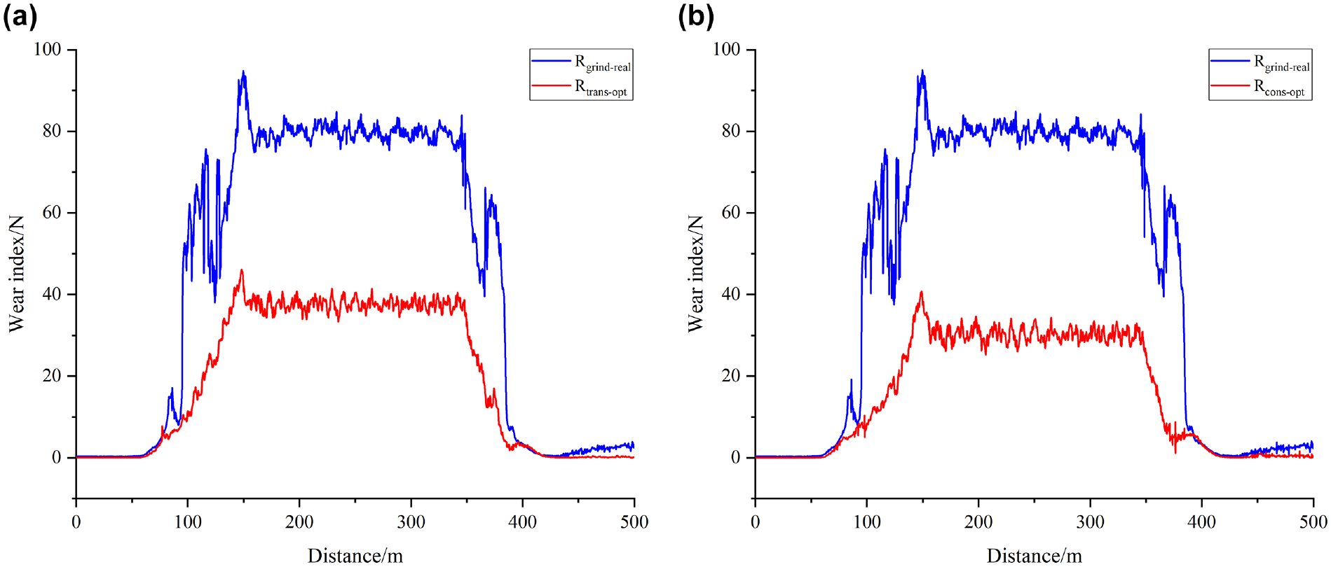
The wear index of the optimized profiles and the measured grinding profile are calculated, respectively. As shown in Figure 17, the wear index of the optimized profiles is significantly smaller than the measured grinding profile. In the transition curve section, compared with $R_{grind - real}$ , the maximum wear index of $R_{trans - opt}$ decreases from 94.7 to 46.2 N, with a decrease of 51.2%, which slows down the rail wear rate. In the circular curve section, compared with $R_{grind - real}$ , the maximum wear index of $R_{cons - opt}$ decreased from 84.8 to 34.2 N, with a decrease of 59.7%, and the rail wear strength decreased significantly.

Figure 17.

Variation curve of wear index with running distance: (a) $R_{grind - real}$ / $R_{trans - opt}$ and (b) $R_{grind - real}$ / $R_{cons - opt}$ .

Surface Fatigue Index

Wheel–rail rolling contact fatigue is a common form of wheel–rail damage, which directly affects the service life of the wheel–rail. Ekberg et al. ( 26 ) use the wheel–rail surface contact fatigue index $F I_{surf}$ to evaluate the rolling contact fatigue characteristics, and its definition is as follows:

F I_{surf} = \frac{\sqrt{{T_{x}}^{2} + {T_{y}}^{2}}}{F_{z}} - \frac{2 π abk}{3 F_{z}}

(31)

where $T_{x}$ and $T_{y}$ are longitudinal creep force and lateral creep force, respectively; $F_{z}$ is wheel–rail normal force; a and b are the short and long half axes of the elliptical contact spots, respectively; and k is the pure shear yield strength of material, where the rail material is U75V (hot-rolled steel), k = 300 MPa ( 27 ).

The magnitude of the surface fatigue index represents the probability of wheel–rail fatigue damage. If the calculated $F I_{surf}$ is greater than zero, it means that it enters the rolling contact fatigue zone of the material, and then rolling contact fatigue may occur. The surface fatigue index of the optimized profiles and the measured grinding profile are calculated. As shown in Figure 18, in the transition curve section, the surface fatigue index of $R_{grind - real}$ has large fluctuations, which is mainly caused by the two-point contact or jump of the contact point when entering the transition curve section. The surface fatigue index of $R_{trans - opt}$ increases smoothly with the running distance without obvious fluctuation. In the circular curve section, compared with the maximum surface fatigue index 0.127 of $R_{grind - real}$ , the maximum after using $R_{cons - opt}$ is 0.026, a decrease of 79.5%. Both kinds of fatigue indexes are greater than zero, and fatigue cracks may appear on the rail surface. However, the probability of fatigue cracks in $R_{cons - opt}$ is significantly reduced, which can effectively extend the rail service life.

Figure 18.

Variation curve of the surface fatigue index with running distance: (a) $R_{grind - real}$ / $R_{trans - opt}$ and (b) R $R_{grind - real}$ / $R_{cons - opt}$ .

Conclusions

In this paper, based on the measured worn profile and grinding profile in the curve section of the Daqin heavy-haul railway, the representative worn profile of different sections is selected by the Frechet distance method as the input condition of the grinding target profile design, which can better show the real wear situation of different sections. The NURBS curve is reconstructed by establishing a multi-objective optimization mode for the worn rail profile of the curve section. Although the wear law of rails in each section of the curve section is different, and the wear position is also very different, by establishing the corresponding optimization design model and continuously optimizing the iteration, the cubic NURBS curve can be used to fit and reconstruct the rail profile curve with high precision, so that a rail grinding profile with good performance is obtained. The optimized grinding profile and the measured grinding profile are compared in multiple directions. The conclusions are as follows.

(1) Compared with $R_{grind - real}$ , the rail grinding amounts of $R_{trans - opt}$ and $R_{cons - opt}$ are reduced by 80.1% and 11.3%, respectively. At the same time, the uniformity of the wheel–rail contact is significantly improved, which can effectively prolong the service life of the rail.

(2) In the studied curve radius and velocity range, the dynamic evaluation index of the optimized grinding profile is significantly reduced, and the curve passing performance is significantly improved.

(3) The wear index and fatigue index of the optimized grinding profiles are significantly reduced in the curve section, which is beneficial to reduce the rail wear and the occurrence probability of fatigue cracks, and effectively improves the service life of the rail.

(4) The contact state of the optimized grinding profile is significantly improved, and the maximum von Mises stress is significantly reduced, which can effectively reduce the side wear of the curved rail.

(5) The finite element analysis of wheel–rail static contact cannot fully reflect the change of wheel–rail contact mechanical properties. In subsequent research, a finite element model of wheel–rail rolling contact will be established for dynamic analysis and verified by test bench and field test.

(6) The method proposed in this paper is only used for the grinding profile design of heavy-haul railway, and does not study other rail profiles. In the future, this method will be used to further study the grinding profile design of high-speed railway rails and turnout.

Footnotes

Author Contributions

The authors confirm contribution to the paper as follows: study conception and design: Fengtao Lin, Wu Chen; data collection: Huafei Pang, Rongkai Tan and Taotao Weng; analysis and interpretation of results: Qin Fang, Zhe Jia, Zihao Zhang and Xin Qian; draft manuscript preparation: Fengtao Lin, Wu Chen. All authors reviewed the results and approved the final version of the manuscript.

Declaration of Conflicting Interests

The author(s) declared no potential conflicts of interest with respect to the research, authorship, and/or publication of this article.

Funding

The author(s) disclosed receipt of the following financial support for the research, authorship, and/or publication of this article: This work was supported by the National Natural Science Foundation of China (grant number 51865009, 52065021), the Jiangxi Natural Science Foundation Project (grant number 20212BBE53024, 20202BABL214028), the Major Disciplines and Technology Leading Talents Training Program in Jiangxi Province (grant number 20213BCJL22040), and the Special Fund Project for Postgraduate Innovation in Jiangxi Province (grant number YC2021-S423).

References

Smallwood

Sinclair

J. C.

Sawley

K. J.

An Optimization Technique to Minimize Rail Contact Stress. Wear, Vol. 144, No. 1–2, 1991, pp. 373–384.

Brandau

Wear Reduction in Light Rail Systems Through Asymmetrical Railhead Profiles. Tribology Series, Vol. 40, No. 2, 2002, pp. 305–316.

Persson

Nilsson

Bik

Lundgren

Iwnicki

Use of a Genetic Algorithm to Improve the Rail Profile on Stockholm Underground. Vehicle System, Vol. 48, 2010, pp. 89–104.

Choi

H.-Y.

Lee

D.-H.

Song

C. Y.

Lee

Optimization of Rail Profile to Reduce Wear on Curved Track. International Journal of Precision Engineering & Manufacturing, Vol. 14, No. 4, 2013, pp. 619–625.

Zong

Dhanasekar

Minimization of Railhead Edge Stresses Through Shape Optimization. Engineering Optimization, Vol. 45, No. 9, 2013, pp. 1043–1060.

Zong

Dhanasekar

Hybrid Genetic Algorithm for Elimination of Severe Stress Concentration in Railhead Ends. Journal of Computing in Civil Engineering, Vol. 29, No. 5, 2015, pp. 1943–5487.

Wang

J. X.

Ren

Z. Q.

Chen

J. J.

Chen

Study on Rail Profile Optimization Based on the Nonlinear Relationship Between Profile and Wear Rate. Mathematical Problems in Engineering, Vol. 6, 2017, pp. 1–12.

Zheng

Qiu

Ren

Sun

Yang

Multi-Objective Optimization of Rail Pre-Grinding Profile in Straight Line for High Speed Railway. Journal of Shanghai Jiaotong University (Science), Vol. 23, No. 4, 2018, pp. 527–537.

Jiang

H. W

Gao

Optimizing the Rail Profile for High-Speed Railways Based on Artificial Neural Network and Genetic Algorithm Coupled Method. Sustainability, Vol. 12, No. 2, 2020, pp. 658–669.

10.

Huang

J. L.

Studu on Heavy-Haul Rail Grinding Profile Optimization and Design Based on Contact Stress Analysis. Southwest Jiaotong University, Chengdu, People’s Republic of China, 2015.

11.

Lin

F. T.

Pang

H. F.

Deng

Z. X.

Design Method of Double Grinding Profile for Curved Rai. Journal of Railway Science and Engineering, Vol. 19, No. 1, 2022, pp. 87–99.

12.

Lin

F. T.

Zou

Design Method of Worn Rail Grinding Profile Based on Frechet Distance. Proceedings of the Institution of Mechanical Engineers, Part F: Journal of Rail and Rapid Transit, Vol. 9, No. 11, 2021, pp. 1–12.

13.

Zhou

Rail Grinding and Optimization of Rail Profile in Curve Section of Railway. East China Jiaotong University, Nanchang, People’s Republic of China, 2014.

14.

Mao

Shen

Curved Rail Grinding Profile Design Based on Rolling Radius Difference Function. Journal of Tongji University (Natural Science Edition), Vol. 46, No. 2, 2018, pp. 253–259.

15.

Tang

Y. L.

Dong

Multi-Objective Optimization Design of Rail Profiles on Curve Tracks of Heavy Haul Railway. Mechanical, Vol. 47, No. 12, 2020, pp. 1–9.

16.

Wang

Prediction on Wheel-Rail Wear and Optimization of Rail Profile for Heavy Haul Railway. Beijing Jiaotong University, People’s Republic of China, 2017.

17.

Wang

S. T.

Study on Griding Profile and Fatigue Life of Rail in Froge Section of NO.18 High Speed Turnout. East China Jiaotong University, Nanchang, People’s Republic of China, 2021.

18.

Piegl. Non-Niform Rational B-Spline. Tsinghua University Press, Beijing, People’s Republic of China, 2010.

19.

Wang

K. W.

The Track of Wheel Contact Points and The Calculation of Wheel/Rail Geometric Contact Parameters. Journal of Southwest Jiaotong University, Vol. 1, 1984, pp. 89–99.

20.

Ren

Z. S.

Vehicle System Dynamics. China Railway Publishing Houses, Beijing, People’s Republic of China, 2007.

21.

Rao

Research on the Measurement of Rail Wear Based on Machine Vision. Chongqing University of Technology, People’s Republic of China, 2017.

22.

Standardization Administration of the People’s Republic of China. GB/T 5599—2019 Specification for dynamic performance assessment and testing verification of rolling stock. Standards Press of China, Beijing, People’s Republic of China, 2019.

23.

Dong

X. Q.

Ren

Z. S.

Z. Q.

Zhu

S. G.

Liu

B. C.

Research on Nonlinear Characteristics and Effects of Equivalent Conicity Curve. Journal of Railways, Vol. 40, No. 11, 2018, pp. 91–97.

24.

Zhou

S. X.

Xue

Zhang

Zheng

Wheel-Rail Rolling Contact Finite Element Analysis of the Wear State on the Curve of Subway Line. Journal of Mechanical Engineering, Vol. 52, No. 12, 2018, pp. 129–135.

25.

Ghonem

Kalousek

J. A.

Eualitative Model to Estimate Rail Surface Failure. Wear, Vol. 97, No. 1, 2016, pp. 65–81.

26.

Ekberg

Kabo

Andersson

An Engineering Model for Prediction of Rolling Contact Fatigue of Railway Wheels. Fatigue & Fracture of Engineering Materials & Structures, Vol. 25, No. 10, 2002, pp. 899–909.

27.

Qian

Wang

B. Y.

J. M.

Effect Analysis of Rail Cant on the Wheel -Rail Contact Behavior of High-Speed Railway. Journal of Railway Engineering, Vol. 35, No. 3, 2018, pp. 18–25.