



Abstract
Existing studies on the heterogeneity in traffic flow have considered either conventional car–truck or conventional vehicle–automated vehicle combinations. Nevertheless, these assumptions are not realistic as there will be possible combinations of cars–trucks and conventional–automated vehicles in the future. This study aims to investigate heterogeneous traffic flow with or without an adaptive cruise control (ACC) system for the pair of a front truck and a rear passenger car. Vissim microscopic traffic simulation software and the HighD dataset were applied. The major findings include the following. (1) The greater the penetration rate of ACC vehicles in the same speed interval, the smaller the space headway of the rear car. (2) Both conventional and ACC cars accelerate or decelerate frequently when their speeds exceed that of the front truck in the car-following state. In the free-flow state, a conventional car keeps a constant speed or accelerates, while an ACC car mainly adopts an acceleration strategy. (3) The variation of speed differences and space headways is smallest when both the front truck and rear car have ACC. (4) The probability of conflicts between the front truck and rear car pair decreases with the increase of market penetration of ACC vehicles. Compared to conventional cars, the rear car equipped with ACC exhibits a lower probability of conflicts. Statistical tests further confirmed the significant differences between any two of the four combinations based on the ACC equipment.
Keywords
Traffic flow is determined by numerous factors, including the number of vehicles of different types and the interactions between them. In recent years, researchers have increasingly focused on the heterogeneity of traffic flow ( 1 – 4 ). An important factor is heterogeneity in vehicle composition, which has significant implications for traffic safety ( 5 ). With the growth of population and economic activities, the proportion of trucks on the road has significantly risen from 7.2% in 1994 to 7.5% in 2004 and 9.2% in 2014. ( 6 ). The mixed traffic flow of passenger cars (hereafter referred to as “cars”) and trucks is also very common on freeways, where they share the same driving environment but differ in their physical and maneuver characteristics. Previous research on mixed traffic flow of cars and trucks categorizes them into four combinations, that is, front and rear cars, front and rear trucks, front car and rear truck, and front truck and rear car pair ( 7 – 9 ).
With the adoption of advanced communication and information technologies in connected and autonomous vehicles (CAVs), the mixed traffic of conventional vehicles and CAVs also makes the analysis of the heterogeneity of vehicles more complex. It is expected that fully automated vehicles will be developed and operated in the future; however, there will be a long transition period before the time comes when all vehicles will be fully automated on all types of roads, in which drivers of partially automated vehicles of varying degrees will be in charge of driving tasks ( 10 ). The advent of adaptive cruise control (ACC) provides an effective transition to the long-term goal of fully automated driving in vehicles ( 11 ). The ACC partially automates the vehicle longitudinal control. In addition to maintaining a preset speed, the ACC can also adjust speed to maintain the distance between the rear vehicle and the front vehicle ( 12 ). The mixed traffic flow between ACC vehicles and conventional vehicles has become inevitable, and many scholars have studied the mixed traffic flow between them. Ding et al. ( 13 ) analyzed the impact of the CAV driving strategy considering multiple front vehicles on the road capacity of mixed vehicle traffic flow. Xie and Liu ( 14 ) investigated the mixed traffic flow of CAVs at various automation levels and conventional vehicles. Sinha et al. ( 15 ) evaluated crash severities and rates for conventional vehicles in mixed traffic flows. However, the impact of ACC vehicles on traffic flow remains uncertain ( 16 ). While theoretical studies have shown that ACC vehicles have the potential to maintain stability and reduce congestion ( 17 , 18 ), recent evidence indicates that commercially available ACC systems may operate in a string unstable manner ( 19 – 21 ). Therefore, it remains imperative to study the impact of ACC vehicles on traffic flow.
One of the most typical risky situations is when a truck is followed by a car. A truck in front of a car often makes the car’s driver uncomfortable and causes frequent lane changes, which greatly increases the crash risk. Weng et al. (
22
) found that such front truck and rear car combinations have the highest rear-end crash risk. Therefore, this paper chooses the pair of the front truck and rear car for this research. At the same time, the ACC system is one of the most popular automated driving applications and an increasing number of new vehicles have been equipped with it in recent years. Nevertheless, existing studies on the heterogeneity in traffic flow considered either only conventional car–truck or solely conventional vehicle–automated vehicle combinations (
11
). These assumptions are not very realistic as there will be various mixtures of cars–trucks and conventional–automated vehicles in the future. Studies on a combination of the two factors are rare but necessary. This study considers that some vehicles are equipped with an ACC system, and there are four main types of vehicles on the road: conventional car (
to explore the impact of the market penetration rates (MPRs) of vehicles equipped with ACC on the interactions between the front truck and rear car, and their effects on macroscopic and microscopic traffic flow indicators;
to analyze the dissimilarities in car-following behaviors of different combinations considering automation (i.e., ACC or conventional) and vehicle types (i.e., cars and trucks).
Methodology
Framework of the Simulation Platform
Microscopic traffic simulation PTV Vissim 2022 was used in this study ( 23 ). The framework of the simulation platform of this paper is shown in Figure 1. Firstly, the HighD dataset was processed to build a basic simulation scenario in PTV Vissim. Then, the data interaction platform between Vissim and MATLAB was built, and the calibration and optimization of the parameters of the car-following model for the conventional vehicle in Vissim are achieved by a genetic algorithm (GA). The control model of the ACC vehicle car-following behavior is calibrated using the OpenACC dataset and is realized by the external driver model application of programming interface (API) using the Vissim simulation software. Finally, different MPRs (0%–75%) are analyzed by adjusting the flow ratio of conventional vehicles and ACC vehicles, with randomly distributed ACC vehicles in the traffic flow, and conducting simulation experiments.
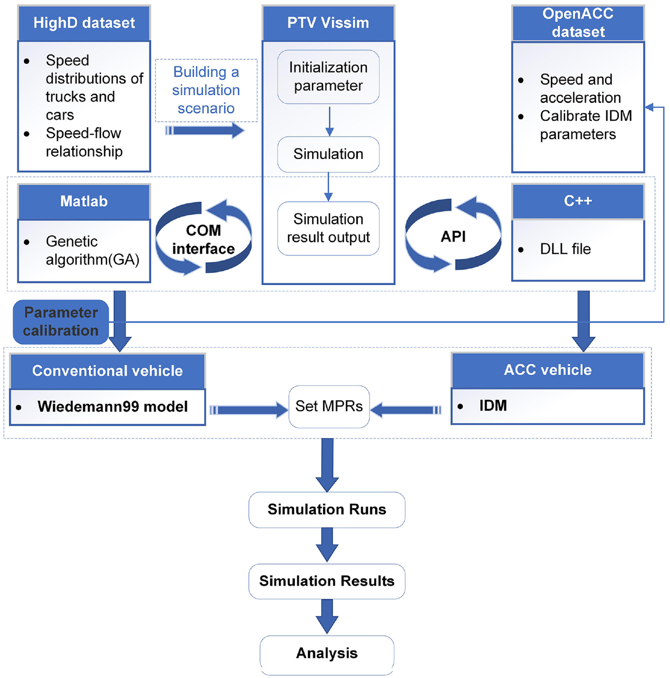
Framework of the simulation platform.
Fundamental Information of Simulation Scenarios
The simulation scenarios used in this study are obtained from the HighD dataset, which is a new dataset of natural vehicle trajectories captured on German autobahns ( 24 ). To meet the input and output requirements of the simulation software and calibration data needs, the data used in this paper are sorted out as follows.
Geometry data: the highway consists of four lanes, with two lanes in each direction. Each lane measures 400 m in length and 4 m in width as observed from the video footage.
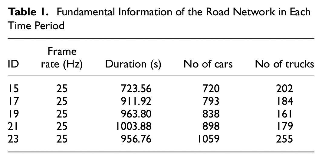
Traffic data: this study extracted five time segments from the dataset, and the fundamental information of the road network in each time period is shown in Table 1. After removing the beginning and end of each time period, the total time is 4325 s (∼1.2 h). The traffic flow of the upper two lanes is 2212 vehicles per hour (vph), and the traffic flow of the lower two lanes is 1963 vph. The average proportion of trucks is 18.5%.
Vehicle speed data: the speed information of different vehicle types during the aforementioned time period was extracted. The speed distributions of cars and trucks are shown in Figure 2.
Fundamental Information of the Road Network in Each Time Period
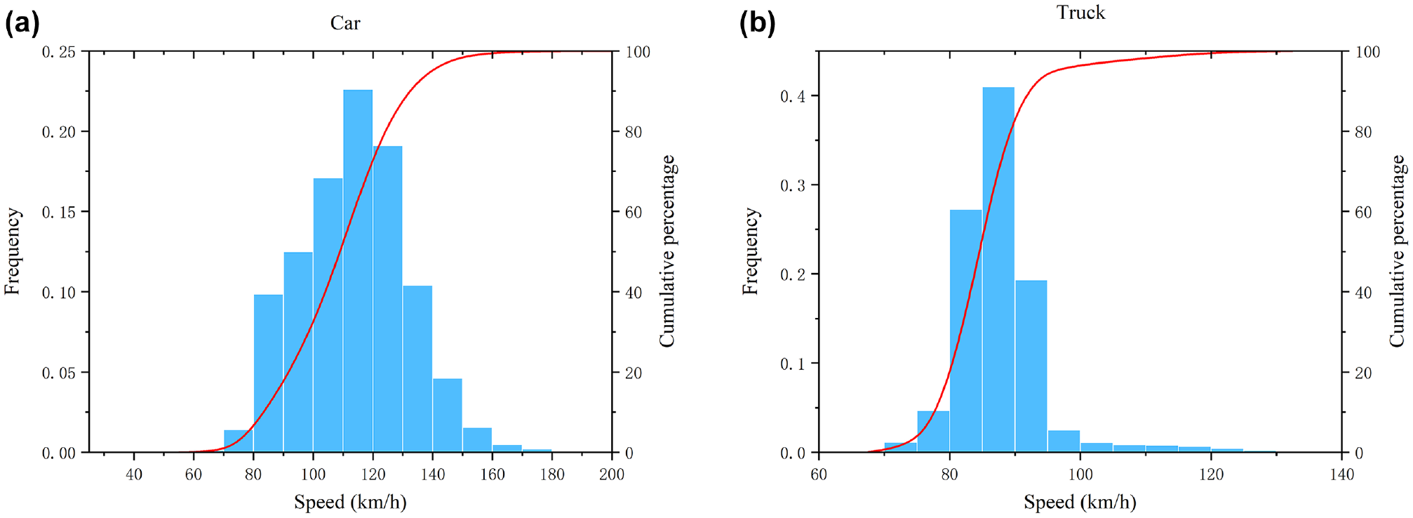
(a) Speed distributions of cars and (b) speed distributions of trucks.
Design of Simulation Scenarios
Based on the HighD dataset, we reproduce the HighD road network scene in Vissim. The simulated road is 400 m long and 4 m wide, consistent with the HighD. A new mixed traffic scenario is constructed by setting the input proportion of different types of vehicles to achieve the replacement of some conventional vehicles with ACC vehicles. Each simulation lasted 4325 s. The traffic flow rate of the upper two lanes is 2212 vph and the traffic flow rate of the lower two lanes is 1963 vph. According to the speed distribution of trucks and cars in HighD, the speed distribution of corresponding vehicles is set in Vissim. The road network will consist of four types of vehicles: conventional car (
In numerous previous studies, the anticipated impacts of ACC systems on traffic flow and stability were generally regarded as positive ( 26 ). However, some researchers ( 27 – 29 ) have uncovered that the currently available commercially ACC systems exhibit string instability. In either case, it is proven that ACC vehicles have effects on the transmission of disturbance to the upstream (whether positive or negative). The Vissim simulation was configured with different MPRs (0%, 25%, 50%, and 75%) for ACC vehicles. The proportion of trucks in both ACC vehicles and conventional vehicles was set at 18.5% to align with the distribution observed in the HighD dataset, while passenger cars accounted for the remaining 81.5%. Then, trajectory information of the four combinations was screened out from the simulation trajectory data for analysis.
Conventional Vehicles
Car-Following Model of Conventional Vehicles
Many car-following models have been developed, which can broadly be categorized into five groups: stimulus-based (Gazis–Herman–Rothery), safety distance (Gipps), desired measures (IDM), optimal velocity (Full Velocity Difference), and psycho-physical models (Wiedemann). These diverse models have been widely applied in traffic flow research. In this study, the selection of the Wiedemann psychology-physics car-following model is based on its consideration of a wider range of psychological and physical factors compared to other conventional vehicle car-following models, including reaction time, acceleration, visual information, and so forth. This enables it to more accurately replicate human driver behavior, and it has been adapted and enhanced by Vissim microsimulation software. Despite having more parameters, the Wiedemann model enables one to simulate a variety of driving scenarios comprehensively. This model was established by Wiedemann ( 30 ). The fundamental concept of this model is based on driving awareness. In other words, when a vehicle approaches the vehicle in front gradually at a high speed, the distance perception threshold judged by the driver would be gradually reached, and then the driver would start to brake. Nevertheless, since the driver cannot estimate the accurate speed of the front vehicle, their speed would continuously decrease to below the speed of the front vehicle. When the speed is outside the lower limit of the perception threshold, the driver would slightly accelerate again until it reaches the perception threshold. The driver’s judgment of distance perception threshold and speed would lead to continuous acceleration and deceleration behaviors.
Calibration of Car-Following Model for Conventional Vehicles
The Wiedemann99 following model consists of 10 main parameters: W99cc0–W99cc9. Considering the sensitivity of parameters to simulation results, this paper selects five parameters (i.e., W99cc1, W99cc2, W99cc3, W99cc4, and W99cc5) that have a great influence on the capacity for calibration. For the conventional vehicle simulation model, the objective function selects the difference measurement method to judge the difference in the field of pattern recognition, that is, the difference between the actual and the simulated flow–speed graph is minimized. The difference measurement method is actually to measure the degree of similarity or coincidence between two identified objects ( 31 ). According to the actual data and simulation output results, the flow–speed diagram is formed, and then the flow–speed diagram is transformed into a binary image. Binary image refers to the value of each pixel in the image being 0 or 255, and the color presented by the pixel in the graph is either black or white.
An integrated Vissim–MATLAB simulation environment is used for parameter calibration. After setting the relevant data of the road network in Vissim, MATLAB can realize the control and data access to Vissim through the COM interface of Vissim. In this study, MATLAB calibrated the model parameters by the GA, and the simulation ran for one cycle after one iteration of the GA. The crossover probability of genes is set at 0.75 and the mutation probability is set at 0.05 in the GA. The number of parameter iterations is set to 50. The image matrix can be used for calculation, and the difference can be obtained by comparing the value of the same position in the image pixel matrix. The parameter corresponding to the minimum difference between the two is the optimal parameter of the model. The calibration results of the car-following model for conventional vehicles are shown in Appendix A.
Figure 3a is the comparison diagram of the flow–speed obtained by the Vissim simulation with the default simulation parameters and the flow–speed obtained by actual data. Figure 3b is the comparison diagram of the flow–speed obtained by the Vissim simulation with the calibrated parameters and the flow–speed obtained by actual data. It is obvious that parameter calibration leads to a better fit between the simulated flow–speed and the actual data.
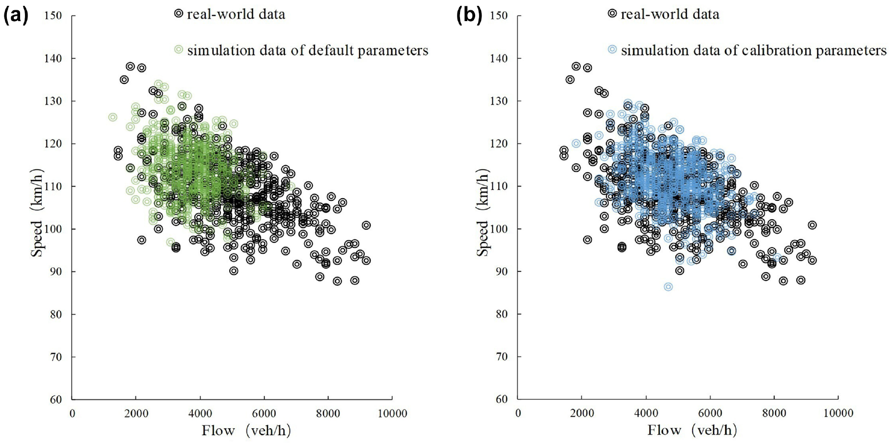
(a) Speed–flow relationship from default simulation and actual data and (b) speed–flow relationship from calibrated simulation and actual data.
In this study, we employed Geoffrey E. Heavers (GEH) statistics, correlation coefficients (CCs), and Theil’s inequality coefficients to substantiate the validity of the calibration results. The GEH statistic is an improved chi-square statistic, which includes relative and absolute differences. It serves as a mean to compare an observed traffic volume with a simulated traffic volume ( 32 ). The definition of the GEH statistic is as follows:

where

where n is the total number of observations,
To better quantify the difference between the simulated and real scenarios, an additional measurement method that provides relative error information is adopted in this paper. Theil’s inequality coefficient, a goodness-of-fit measure developed by Theil in his work on economic forecasting ( 34 ), offers modelers additional information about the nature of the error between the real measurement and the simulated value. Theil’s inequality coefficient is defined as follows:
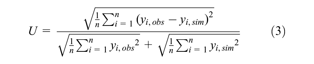
where n represents the number of observations and
Previous study suggests that in 85% of cases, when the GEH value is less than 5, the simulated volume exactly replicates the observed volume ( 35 ). The results show that more than 88% of cases have a GEH value of less than 5 after calibration, which is only 65% of cases for the default parameters. To facilitate comparison, traffic flows were aggregated into 1-min intervals to obtain 72 groups of observed and simulated values. The finding of a previous study indicates that the CC value of 0.85 is considered acceptable for model calibration ( 34 ). The CC value after calibration is 0.88, while the default parameter is only 0.61. Meanwhile, Theil’s inequality coefficient exhibits a decrease from 0.16 to 0.09 after calibration, indicating an enhanced ability of the calibrated parameters to accurately depict real-world traffic flows. The standard deviation of speed was calculated for each vehicle in the HighD dataset and the calibrated simulation model. The resulting scatter plot and distribution for the standard deviation of speed are presented in Figure 4. The similar distribution further supports the ability of the calibrated simulation model to accurately replicate the real-world scenario.

The standard deviation of speed for each vehicle in the HighD dataset and the calibrated simulation model.
Adaptive Cruise Control Vehicles
Car-Following Model of ACC Vehicles
More than 30 years have passed since ACC-equipped vehicles were first introduced onto the market. Despite extensive research work, the operational design of these systems remains almost a black box for the research community, because of intellectual property protections. The limited number of experimental testing activities involving ACC vehicles also makes it difficult to understand the degree of similarity in implementation logic used by different manufacturers or available in different vehicle types ( 36 ). Consequently, most current studies usually use existing models to simulate ACC vehicles to maximize their similar driving behaviors. In this paper, the IDM and ACC model of the PATH Program of Transportation Research Institute of the University of California, Berkeley ( 37 ), were selected to describe the following behavior of ACC vehicles.
Extensive researches have been conducted by the PATH Program of Transportation Research Institute of the University of California, Berkeley, on the traffic flow model for the ACC vehicle, and their car-following model of vehicles equipped with ACC based on real experimental data has been widely recognized and applied. The model is shown in Equation 4:

where
Note that while the IDM was originally built to model human-driven vehicles, it has been widely applied in modeling autonomous and partially autonomous vehicles in previous researches (
38
–
41
). The IDM has been proven to be the closest to the real automated vehicle following model (
18
,
42
). The IDM can simulate the speed oscillation and start and stop the process of the intelligent connected vehicle in the running process, and output acceleration and deceleration files close to the real ones. Current simulation studies have proved that, compared with other car-following models, the IDM can simulate the best driving behavior of automated vehicles, and thus many safety studies have taken the IDM as the microsimulation car-following model (
43
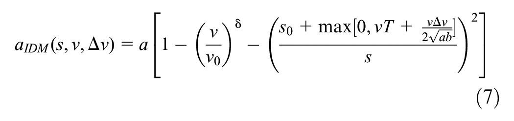
). The IDM acceleration is a continuous function that includes different driving modes at all speeds in highway traffic and urban traffic. In addition to considering the bumper-to-bumper gap


where
Calibration of the Car-Following Model for ACC Vehicles
To select the optimal parameter values of the car-following model of ACC vehicles, we calibrated parameters using actual commercial ACC vehicles to produce the most appropriate following behavior. The OpenACC database ( 44 ) is an open database of different following experiments involving 28 vehicles, 22 of which were equipped with state-of-the-art commercial ACC systems. This paper uses data from a test on a public road in northern Italy on October 27, 2020. During the whole experiment, the car-following order was the same and the follower vehicle was driving at all times with the ACC on.
It is noted that the reason for the calibration method differing from that of conventional vehicles is because of the dataset used for parameter calibration. As mentioned above, the HighD dataset is a long-term collection of vehicle trajectory data within a fixed road network, involving thousands of vehicles. If only the trajectory data of a single vehicle is extracted for calibration, the results may be inaccurate because of insufficient driving time. Therefore, we extracted speed distribution, acceleration distribution, space headway distribution, and other vehicle characteristics of conventional cars and trucks from the HighD dataset and set them respectively in Vissim. Then, we conducted collective calibration on conventional cars and trucks using vehicles throughout the entire road network. The OpenACC dataset was collected for the long-term tracking of a single vehicle or a pair of vehicles. The trajectory data possess the attributes of prolonged duration and heightened precision in capturing the fixed vehicles’ behavior, so it would be more appropriate for the calibration of ACC cars and trucks respectively. Therefore, the GA is employed for calibrating the parameters of a car equipped with ACC; the gene crossover probability was set at 0.75, while the gene mutation probability was set at 0.05. The number of parameter iterations was set at 100, and each model calibration experiment was repeated 10 times to verify whether the algorithm converges to the same minimum value in each repetition. Table 2 presents the lower and upper limits of calibration parameters for both models. The optimization objective is to minimize the normalized root-mean-square error
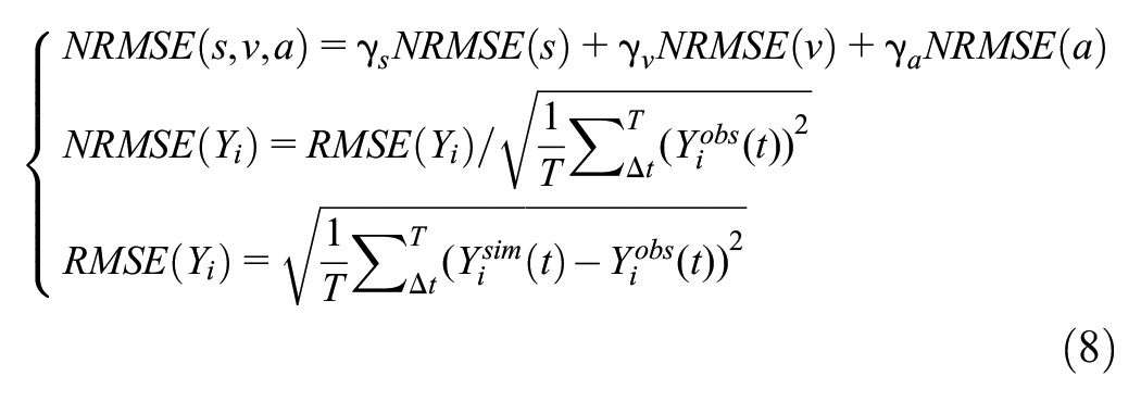
where
Lower and Upper Limits of Calibration Parameters for the Two Models
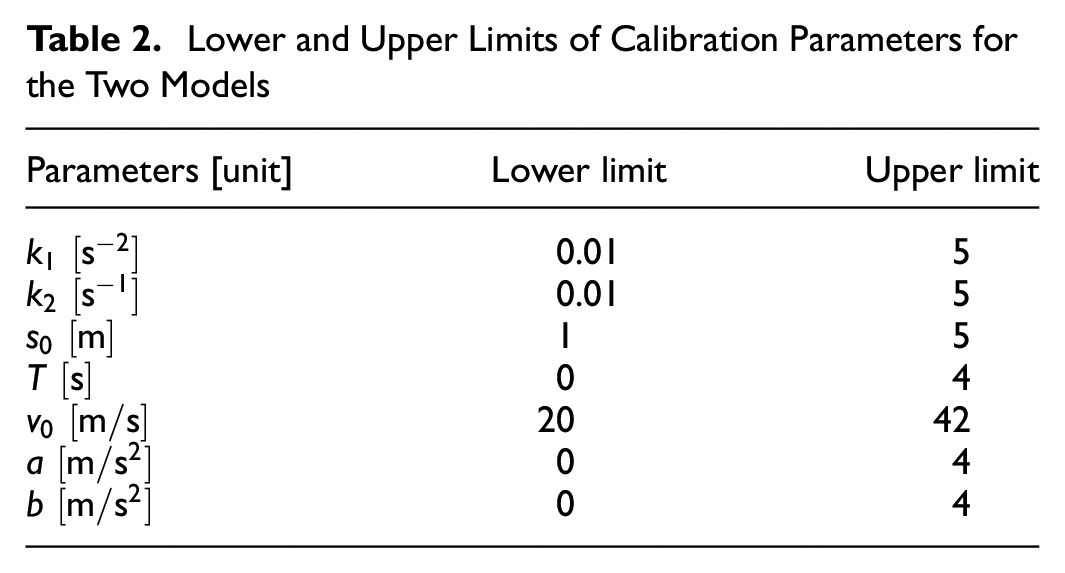
Figure 5a shows the changes of simulated acceleration and real acceleration over time after calibration, while Figure 5b shows the change of simulated velocity and real velocity with time after calibration. The
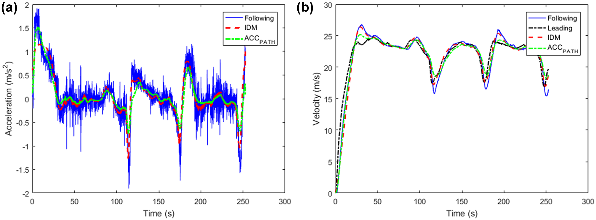
(a) Real and simulation data on acceleration of the adaptive cruise control (ACC) car and (b) real and simulation data on velocity of the adaptive cruise control (ACC) car.
Implement the Car-Following Model for ACC Vehicles in Vissim
The external driver interface of Vissim can modify the vehicle’s behavior parameters, including speed, acceleration, position, lane change signal, and other relevant information. This allows for changes in driving behavior and improves the model through the output data. After the external driver model is imported into Vissim through the interface, the vehicle type controlled by the model will not be dominated by the internal driving behavior of Vissim, but only subject to the imported driver model behavior parameters. This paper adopted the C++ programming language to develop an IDM program. The external driver model algorithm must be compiled in the form of a dynamic link library (DLL) and imported into Vissim for invocation. Figure 6 shows the interaction flowchart of the external driver model and Vissim.
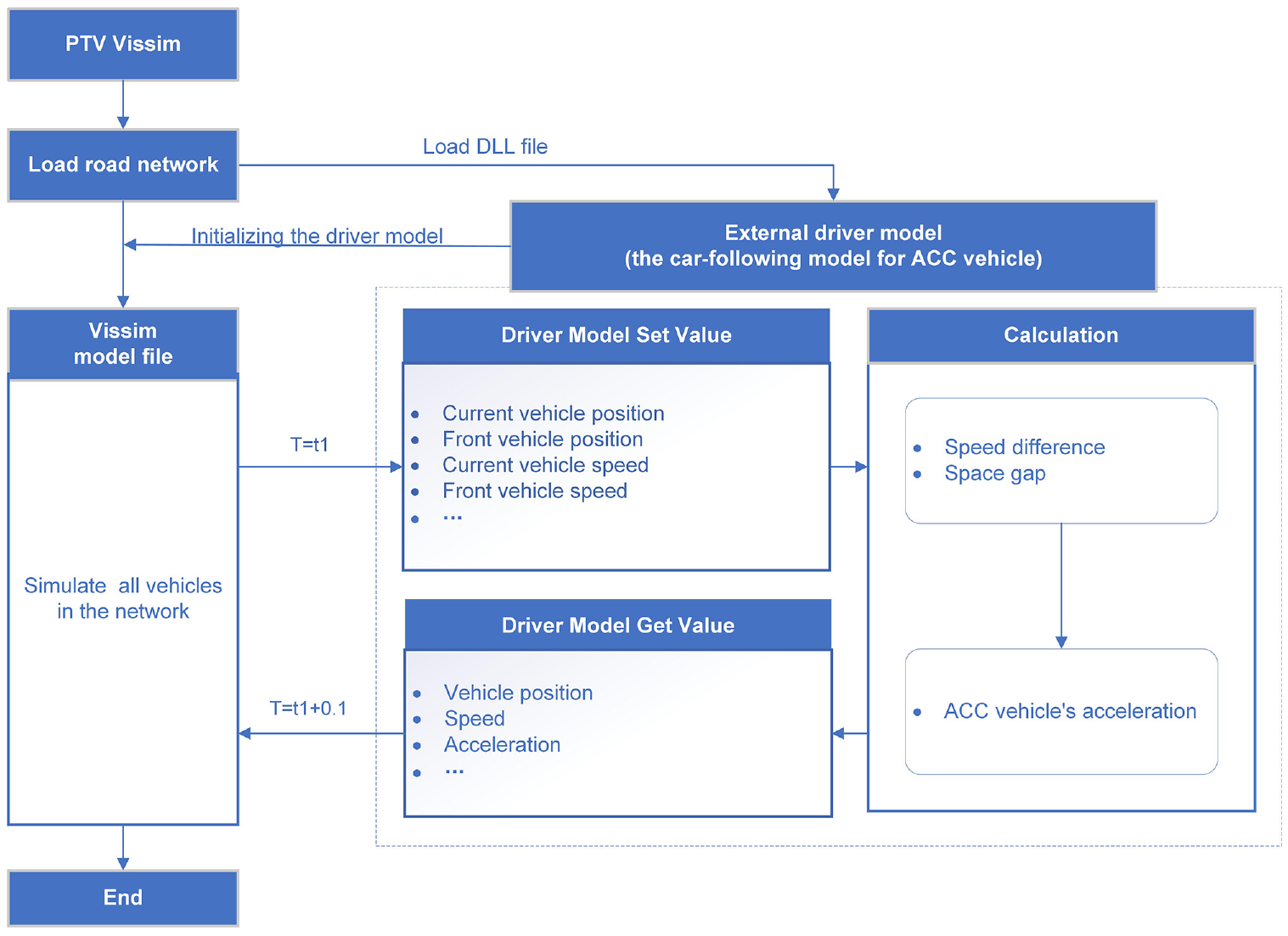
Flowchart of interaction between the external driver model and Vissim.
Sensitivity Analysis of the Car-Following Model
A sensitivity analysis is necessary to investigate the impact of parameter changes in the traffic microsimulation model on the simulation results, thereby providing a more scientifically grounded basis for the parameters selected. We employed a quantitative analysis approach for evaluation, wherein we select a parameter as the target parameter and adjusted it by a predetermined step size while keeping all other parameters constant. Experimental data obtained from each adjustment are recorded, enabling us to generate simulation results with varying parameter values. Finally, we analyzed the impact of each parameter on the results using a sensitivity coefficient. If the influence degree is high, the sensitivity is high.
Suppose there is a simulation system, where the system output evaluation index

where
Calibrated Values, Value Ranges, and Adjustment Steps of the Parameters
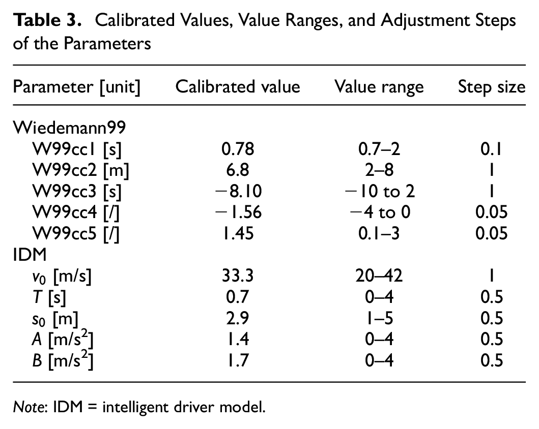
Note: IDM = intelligent driver model.
The research findings primarily depend on the space headway and relative speed of the vehicle combination. These two parameters are extracted from the experimental data, and their average values are utilized as evaluation indices. The sensitivity coefficient of 10 parameters to each evaluation index was calculated using Equation 9, as presented in Table 4.
Sensitivity Coefficient of the Parameters

Note: IDM = intelligent driver model.
By comparing the sensitivity coefficients of different parameters in Table 4, it can be seen that in the Wiedemann99 model, the sensitivity coefficients of parameters to the space headway from large to small are W99cc1, W99cc2, W99cc3, W99cc5, and W99cc4, and the sensitivity coefficients of parameters to the relative speed from large to small are W99cc4, W99cc5, W99cc3, W99cc1, and W99cc2. In the IDM, the sensitivity coefficients of parameters to space headway from large to small are T,
Results and Discussion
Effects of Market Penetration Rates
This section analyzes the space headway of the combination of a front truck and rear car under different MPRs of ACC vehicles and extracts the space headway of all the combinations of the front truck and rear car from the dataset. The space headway, defined as the sum of the space gap and vehicle length, represents the distance between the front bumpers of the leading and following vehicles (Figure 7).
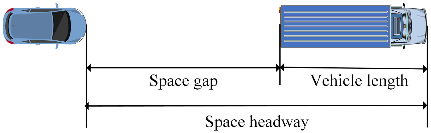
Illustration of space headway.
Space headway was set to 5 km/h intervals according to the speed of the rear car. The average speed of each speed interval represents the corresponding speed range. Figure 8 shows the average space headway of each speed interval in the speed range of 25–85 km/h, reflecting the effect of the rear car speed on its space headway. It can be seen that the space headway of 75% MPR is the smallest, while the space headway of 0% MPR is the largest. In the same speed interval, the space headway is roughly negatively correlated with the MPRs. Interestingly, most of the previous studies suggest that human drivers tend to maintain a smaller headway compared to ACC vehicles. This finding appears inconsistent with our study results, which could be because only one specific following combination (the pair of a front truck and rear car) is extracted in this study, representing only a small fraction of all possible following combinations on the entire road network. In addition, it may also be influenced by the different sources of calibration datasets for these two vehicle types. This observation was supported by a recent study by Apostolakis et al. ( 49 ), where they used the OpenACC dataset and found that ACC systems exhibit smaller (absolute) values of time and space headways, greater stability, and better distribution than those observed among human drivers.
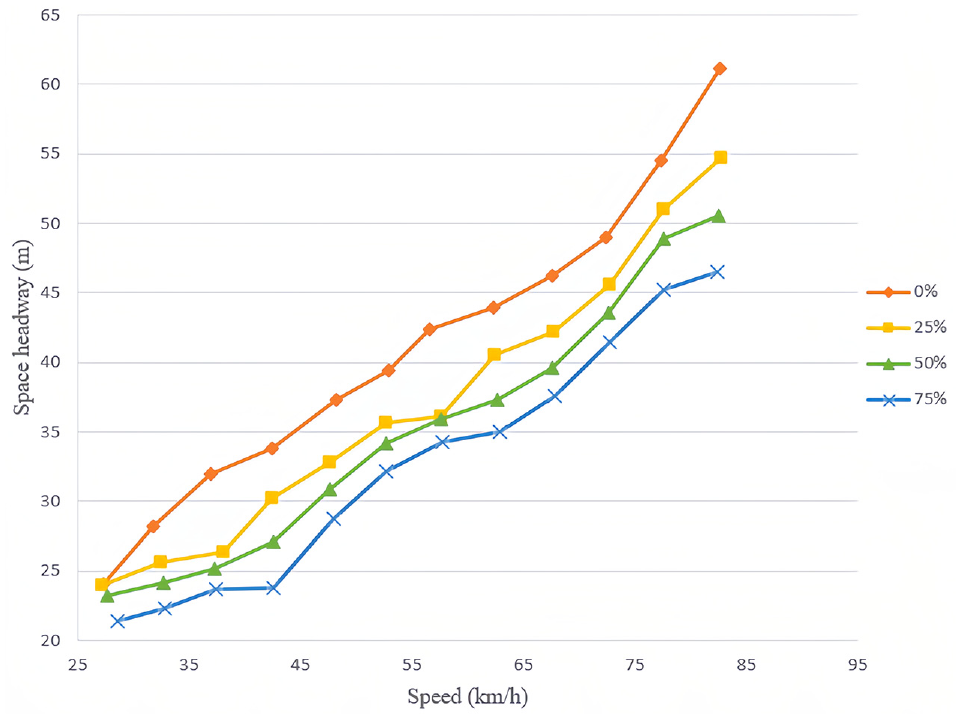
Average space headway of each speed interval.
To compare the difference in space headway between combinations under different MPRs, a two-sample t-test was performed on two independent samples with unknown standard deviations. The tested pairs are (1) 0% versus 25%; (2) 0% versus 50%; (3) 0% versus 75%; (4) 25% versus 50%; (5) 25% versus 75%; and (6) 50% versus 75%. Because of space limitations, Table 5 shows only the 0% versus 75% test results. The null hypothesis was that the space headway of 0% MPR is equal to the space headway of 75% MPR. The results in Table 5 reject the null hypothesis showing that the space headway between 0% and 75% MPR is significantly different except for the speed intervals of 25–30 and 30–35 km/h. Five other pairs were also tested. It was found that there is no difference between the five cases in the speed interval of 25–30 km/h, indicating that the MPRs have little effect on the space headway at lower speeds. There is no difference between 25% versus 50%; 25% versus 75%; and 50% versus 75% in the speed intervals of 35–40 and 55–60 km/h, which may be related to the small sample sizes in these two speed intervals (all less than 20, while the others are more than 40). Since 83% of cases were found to be significantly different at the 95% confidence level, it can be concluded that there are significant differences in space headway for different MPRs, except in some low-speed intervals.
The t-Test for 0% versus 75% Market Penetration Rates (MPRs)
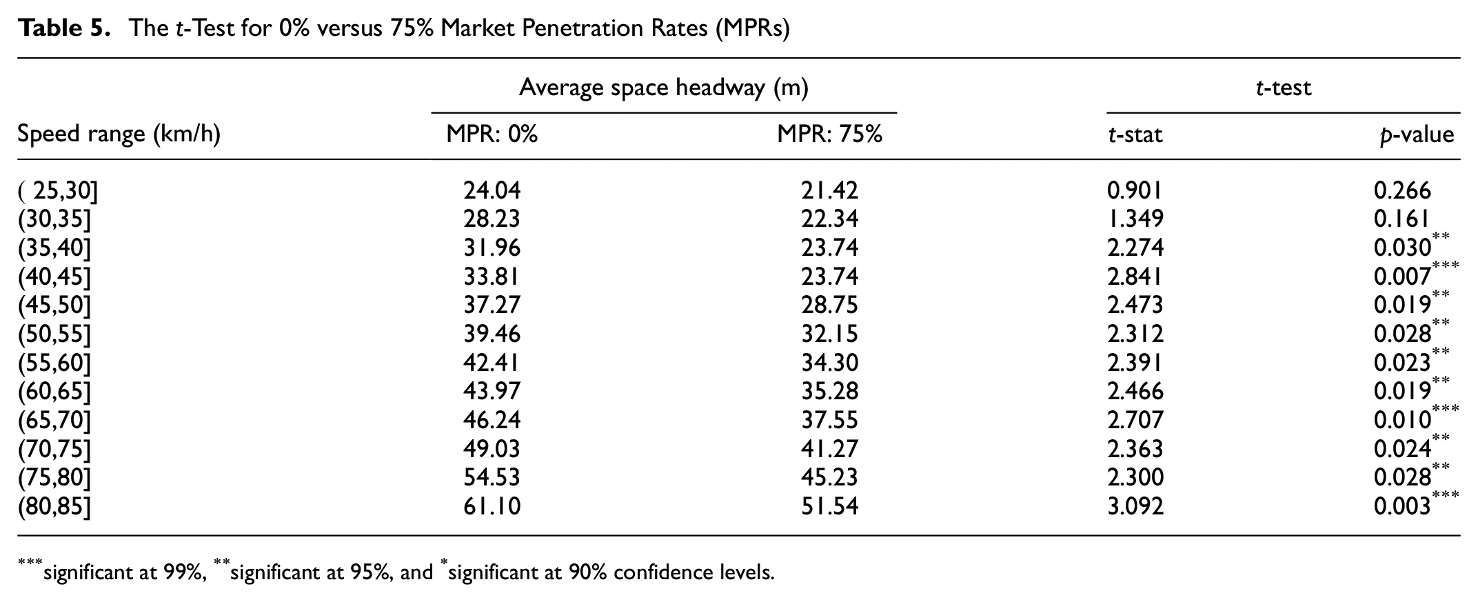
significant at 99%, **significant at 95%, and *significant at 90% confidence levels.
Analysis of Acceleration and Deceleration of Vehicles
According to the distance between two vehicles, the driving behavior of the rear car can be divided into two categories: free-flow and car-following. When the distance between two vehicles exceeds a certain threshold, the rear vehicle is almost unaffected by the front vehicle and operates in a free-flow state, while when the distance falls below this threshold, it enters a car-following state ( 50 ). In the car-following theory, the car-following state is typically determined based on the absolute value of the relative speed. This quantitative approach determines the driving state of the vehicle by using the absolute value of the speed difference between the front and rear vehicles along with the change rule of the space headway. When the space headway is small, the relative speed is dense near the zero axis; as it increases, the relative speed gradually rises. Therefore, it is believed that the speed difference between the front and rear vehicles can reflect the running condition of the two vehicles to a certain extent. The curve of relative speed along with the distance between two vehicles can be divided into two stages: the rising stage and the horizontal stage. The turning point of the absolute value of relative speed from linear growth to horizontal fluctuation is considered as the turning point of the change from a car-following state to free-flow state. The real-world data (HighD dataset) space headway was grouped with an interval of 5 m, and the relationship between space headway and absolute relative velocity was obtained as shown in Figure 9. It can be seen from the figure that the absolute relative speed increases almost linearly with the increase of space headway between 0 and 112 m; above 112 m, the relative speed fluctuates within a certain range, which satisfies traffic flow theory ( 41 ) in that the car-following behavior occurs in space headway between 0 and 100 or 0 and 125 m. Therefore, 112 m is used to distinguish the driving behavior of the rear car, and it is believed that vehicle car-following behavior is affected by the space headway and relative speed between the front and rear vehicle. The turning point value is denoted as the steady space headway.
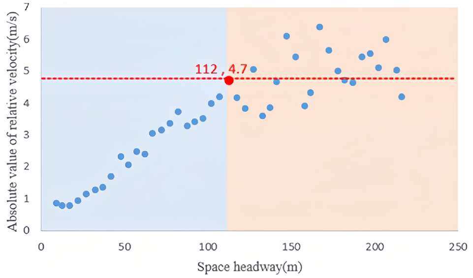
Relationship between the space headway and absolute relative velocity.
To simplify the analysis, and given that the sample number difference of each vehicle combination at 50% MPR is small, only vehicle combinations at 50% MPR are included in the analysis. For each vehicle combination, it was divided into four following cases based on the space headway and relative speed (e.g., the space headway is greater than the steady space headway and the speed of the rear car is less than or equal to the front truck is considered as one case). Table 6 shows the driving actions (acceleration, constant speed, and deceleration) of the rear car for each vehicle combination in each situation. Because it is difficult to keep the speed absolutely unchanged during the driving process, a range from −0.05 to 0.05 m/s2 is considered as constant speed, values greater than 0.05 m/s2 indicate acceleration behavior, and values less than −0.05 m/s2 indicate deceleration behavior.
Car-Following Behavior Choice for Each Vehicle Combination in Each Situation

Very few cases (n = 3).
The study designated four situations: situation 1 (
According to the results in Table 6, the typical driving behavior of the four vehicle combinations is significantly different. For example,
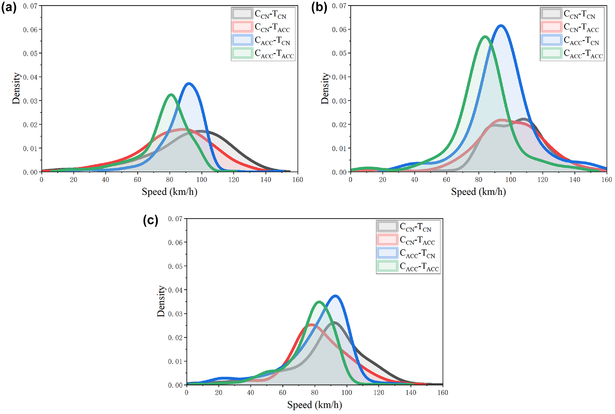
The speed density distribution for each driving action: (a) acceleration, (b) constant speed, and (c) deceleration.
It is observed from Figure 10 that the speed density distribution of ACC vehicles exhibits similarity under both acceleration and deceleration conditions, while the density in the medium speed range (70–100 km/h) significantly increases during constant speed behavior. In contrast, conventional vehicles display a notable difference in their speed density distribution between acceleration and deceleration scenarios: there is more concentrated speed distribution in the deceleration scenario. A comprehensive analysis reveals that ACC vehicles exhibit more concentrated speed distribution compared to conventional vehicles, which demonstrate a more dispersed pattern.
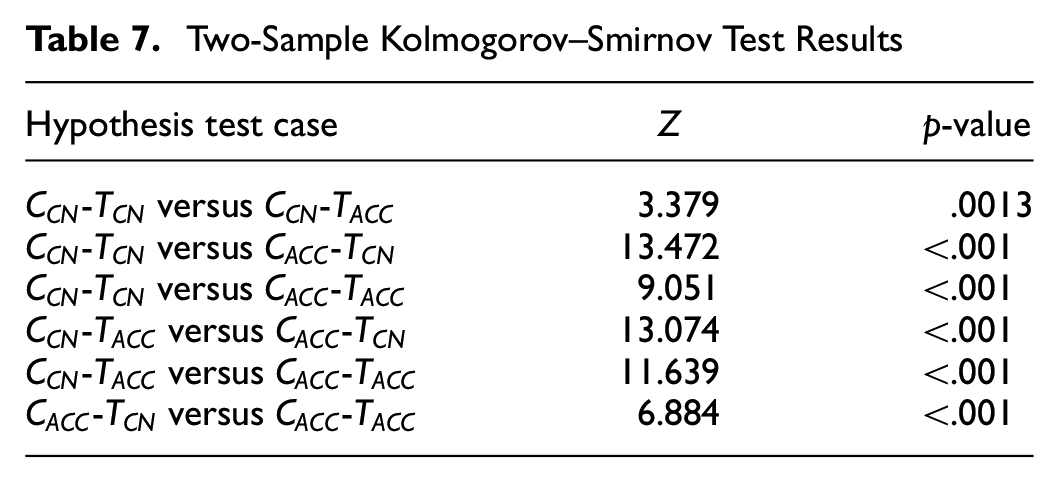
To verify the statistical difference between different vehicle combinations, the acceleration distribution of any two groups of vehicle combinations was tested by a two-sample Kolmogorov–Smirnov (K-S) test. This is a nonparametric test that does not rely on any assumptions about the variable distribution ( 51 ). The null hypothesis was that the acceleration distributions are the same and the alternative hypothesis was different, and the test was conducted at a 95% confidence level. The test results of each group are shown in Table 7. The results indicate that all null hypotheses were rejected, providing evidence of statistically significant difference in the acceleration distributions between any combinations.
Two-Sample Kolmogorov–Smirnov Test Results
Plotting of Speed Difference and Space Headway Analysis
The most effective approach to analyzing car-following behavior is by plotting the space headway and speed difference ( 52 ). This section considers the relationship between the speed difference and the space headway between the front and rear vehicles in the four combinations. Speed difference was defined as the speed of the rear car minus the speed of the front truck. Space headway was defined as the distance between the front bumpers of the front and rear vehicles. Similar to the section of Analysis of Acceleration and Deceleration of Vehicles, only vehicle combinations at 50% MPR are selected for analysis in this section. Figure 11 shows the relationship between the speed difference and the space headway among the four combinations based on the ACC equipment. The graphs are drawn to the same scale for comparison, with the vertical axis indicating the speed difference and the horizontal axis indicating the space headway.
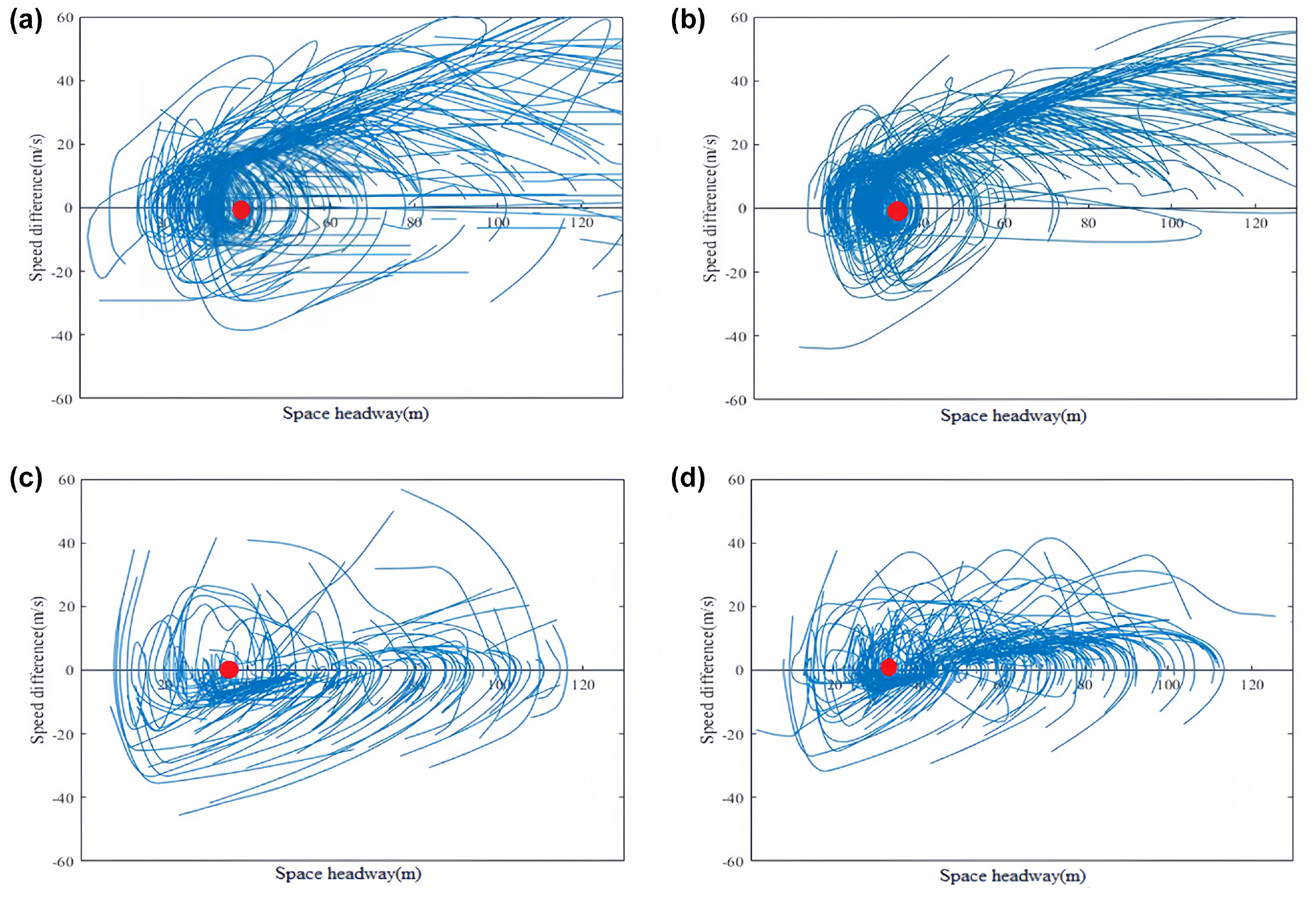
Relationship between the speed difference and the space headway in the four combinations: (a)
Figure 11 shows that when the rear car is equipped with ACC, the range of speed difference is narrower than that when the rear car is conventional. In addition, it is observed that the space headway tends to concentrate or spiral toward a point, which can be interpreted as the desired space headway of the vehicle (
52
,
53
). It is also found that the desired space headway of each type of vehicle combination is not a constant, but, in fact, but oscillates (drifts) around the desired space headway. A comparison reveals that in the specific combination of the front truck and the rear car, the ACC car seems to have a smaller desired space headway than the conventional car. This finding further explains the observed larger space headway at low MPRs. The variation of speed difference from large to small is
To show that there are statistical differences in the distribution of speed difference and space headway between different combinations, two-sample K-S tests were performed for combinations of any two groups. The null hypothesis was that the distribution is the same and the alternative hypothesis is different. The results in Table 8 indicate that all null hypotheses are rejected (p < 0.001). This implies that there are significant statistical differences in the distribution of speed difference and space headway among different combinations based on the ACC equipment.
Two-Sample Kolmogorov–Smirnov Tests for Any Two Groups of Combinations

Safety Evaluation
Neither the HighD dataset nor the OpenACC dataset reported crashes related to critical safety, and thus most vehicles on our network exhibit normal car-following behavior. In microsimulation software, surrogate safety assessment measures (SSAMs) are commonly employed as an indicator for assessing collision risk. To further analyze the safety effects of different MPRs and combinations based on the ACC equipment, this section evaluates traffic conflicts based on time-to-collision (TTC). TTC has been widely used because of its simplicity and reliability in evaluating rear-end collisions. The TTC defines the time remaining before a collision if the involved pair of vehicles continue to maintain their speeds and trajectories. TTC can be calculated according to Equation 10:

where

where
Probability of Conflicts by Market Penetration Rate (MPR)

Note: TTC = time-to-collision.
Probability of Conflicts by Combination (Market Penetration Rate = 50%)
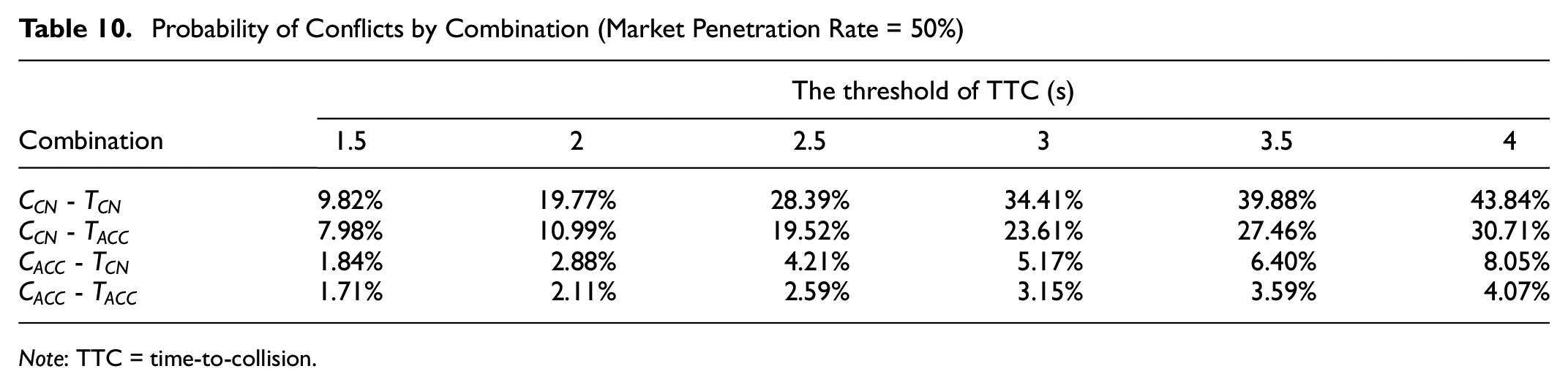
Note: TTC = time-to-collision.
From Table 9, it is observed that the probability of conflicts between the front truck and rear car pair decreases with the increase of the MPR of ACC vehicles. Although the probability of conflicts from 0% to 50% MPR is reduced, the amplitude of change is not very significant, especially when the TTC threshold exceeds 2 s. The probability of conflicts of 75% MPR is significantly smaller than that of the other MPRs. This indicates that with the increase of MPR of ACC vehicles, the probability of conflicts between the front truck and rear car pair can be effectively reduced, and the safety of such combinations can be improved. As depicted in Figure 4, the standard deviation of speeds for 87% of the vehicles in the HighD dataset is less than 6 km/h, indicating a predominantly stable driving behavior. Therefore, the microscopic model has fewer disturbances and it is reasonable to assume that most of the vehicles in this study are in normal car-following conditions. Apostolakis et al. ( 49 ) found that platoons of ACC vehicles are unstable under large perturbation, while their variance is minimal under normal car-following conditions, which is consistent with the conclusion of this study.
Table 10 shows the probability of conflicts by combination when the MPR is 50%. It indicates that the probability of conflicts is lower when the rear car has ACC compared to that when the rear car does not have it. As expected, the probability is the highest when both the car and truck are without ACC, while it is the lowest when both the car and truck have ACC. The result suggests that safety can be greatly improved with ACC of the rear car. It also showed that the front truck’s ACC equipment can reduce conflicts but the contribution of the rear car’s ACC to safety is more obvious. Wen et al. ( 55 ) obtained similar research results.
Conclusions
This paper analyzed the driving behavior characteristics of four different combinations of a front truck and rear car considering the ACC equipment. The key findings from this study are as follows.
The majority of the samples (83%) showed significant differences in space headway and speed of the four different MPRs (0%, 25%, 50%, and 75%). A smaller space headway between the front truck and the rear car is observed when the penetration rate of ACC vehicles is higher in the same speed interval.
A conventional car accelerates and decelerates frequently when its speed exceeds that of the front truck in the car-following state, while it keeps a constant speed or accelerates in free-flow. ACC vehicles also accelerate and decelerate frequently when their speed exceeds the front truck in the car-following state, while the acceleration strategy is mainly adopted in the free-flow state.
The variation of speed differences is the largest when the front truck and rear car are without ACC, and it is the smallest when both are with ACC. The variation of the space headway has the same trend.
The probability of conflicts between the front truck and rear car pair decreases with the increase of the MPR of ACC vehicles. The probability of conflicts is lower when the rear car is equipped with ACC than that when the rear car is conventional.
Previous studies have demonstrated that speed difference, variation of space headway, and acceleration/deceleration behaviors have effects on real-time safety risks ( 56 – 59 ). This study revealed that the ACC equipment has considerable impacts on behaviors (i.e., speed difference, variation of space headway, and acceleration/deceleration) when a truck is followed by a car. Along with the safety evaluation using a surrogate safety measure (i.e., TTC), we conclude that the ACC equipment can significantly enhance traffic safety.
Although this study identified key findings above, further investigations are needed in the future. Firstly, since neither of our calibration datasets for car-following models reported crashes, the aforementioned conclusions of this study were drawn under normal car-following conditions. Therefore, additional research is needed to explore critical safety situations in the future. Secondly, lane-changing behavior adopted the default model of Vissim in this study. Taking a specialized lane-changing model of ACC vehicles into consideration will make the simulation more realistic and comprehensive. Thirdly, freeway data from Germany was used but it is still questionable whether the results are applicable to other countries. Thus, it is necessary to collect data from different countries to analyze and compare. Fourthly, in the sensitivity analysis of the following model, in addition to changing parameters individually, different combinations of all parameters in the following model need to be analyzed to find out which parameter combinations have the greatest impact on the research results. Lastly, the IDM parameters of trucks in this paper were based on past research. This is because trajectory data of CAVs from the real-world are limited at this point, and those of CAV trucks are particularly rare. Once sufficient real-world CAV data becomes available, it will be necessary to adjust the IDM parameters with this data.
On the basis of this study, we can consider the impact of the proportion of trucks in traffic and the market penetration of vehicle automation on mixed traffic flow in future studies. At the same time, considering the communication between vehicles (V2V), there will be more vehicle platooning on the road in the future. It is thought that the position of a truck in the platoon might have significant effects on the string stability of the fleet and eventually the entire traffic flow.
Supplemental Material
sj-docx-1-trr-10.1177_03611981231223982 – Supplemental material for Effects of Adaptive Cruise Control System on Traffic Flow and Safety Considering Various Combinations of Front Truck and Rear Passenger Car Situations
Supplemental material, sj-docx-1-trr-10.1177_03611981231223982 for Effects of Adaptive Cruise Control System on Traffic Flow and Safety Considering Various Combinations of Front Truck and Rear Passenger Car Situations by Jun Bai, Jaeyoung Lee and Suyi Mao in Transportation Research Record
Footnotes
Author Contributions
The authors confirm contribution to the paper as follows: study conception and design: J. Bai, S. Mao; data collection: J. Bai; analysis and interpretation of results: J. Bai, J. Lee; draft manuscript preparation: J. Bai, J. Lee. S. Mao. All authors reviewed the results and approved the final version of the manuscript.
Declaration of Conflicting Interests
The author(s) declared no potential conflicts of interest with respect to the research, authorship, and/or publication of this article.
Funding
The author(s) disclosed receipt of the following financial support for the research, authorship, and/or publication of this article: This research was sponsored by: (1) the Advanced Multidisciplinary Project of Central South University under Grant (No. 2023QYJC016); (2) the National Key R&D Program of China under Grant (No. 2020YFB1600400); (3) the Innovation-Driven Project of Central South University under Grant (No. 2020CX013); (4) the Hunan Provincial Innovation Foundation for Postgraduate under Grant (No. CX20210235); (5) the Fundamental Research Funds for the Central Universities of Central South University under Grant (No. 2021zzts0166); (6) the China Scholarship Council under Grant (No. 202106370107).

Data Accessibility Statement
The data would be available by application to the corresponding author
Supplemental Material
Supplemental material for this article is available online.
References
Supplementary Material
Please find the following supplemental material available below.
For Open Access articles published under a Creative Commons License, all supplemental material carries the same license as the article it is associated with.
For non-Open Access articles published, all supplemental material carries a non-exclusive license, and permission requests for re-use of supplemental material or any part of supplemental material shall be sent directly to the copyright owner as specified in the copyright notice associated with the article.
