Statistics and Genealogy: A Match Made in Heaven? The Forecasting and Inference Tool,an Application of the Central Limit Theorem in Genealogical Research

Introduction

Experience suggests that genealogy enthusiasts often have an aversion to numbers. The division between humanities and the hard sciences is an old one and sometimes seen almost as a feud between long-time enemies.

The objective of this article is to try to begin to (at least partially) heal this division by showing how an application of statistics may be of great interest, and also, possibly, more importantly, be of great use in the field of genealogical research. Indeed, much genealogical research can be optimized by improved estimates for the years of birth, marriage, or death of the subjects being investigated. This is an often unknown variable for the genealogist, who may choose either to adopt a “brute force” approach, looking at all the possible registers year by year, tracking subjects from the cradle to the grave, or somehow estimate the most likely year in which the event occurred, and begin looking from there.

The central limit theorem, a very important finding in statistics, may be used to predict the year in which such events are most likely to have occurred with greater precision. This paper presents the Forecasting and Inference Tool (FAIT), an instrument that, by relying on this theorem and on the most accurate empirical data available in the history and cliometrics literature, suggests to genealogists the best place to begin searching for records.

The remainder of this paper is organized as follows: the next section suggests why a marriage between statistics and genealogy may be useful to practitioners of the latter; section three presents (in layman's terms) the central limit theorem; the fourth section suggests some applications of the theorem in typical genealogical problems; the fifth explains how we operationalized the data used in the instrument; the sixth explains how to use the FAIT; and the seventh concludes.

Are Statistics Useful for Genealogy?

Statistics has been defined as “the science of decision taken in conditions of uncertainty.” ¹ Indeed, the declared objective of this science is to reduce the available information on a given subject, keeping only the most important data and then using them to take the best possible decision. Indeed, one aim of statistics is to reduce the complexity of the world into something that human beings, with our reduced ability to process data, can digest without getting confused by the vast amount of information that reality has to offer us. For instance, a geographical map may be viewed as a statistical operation: it reduces a large amount of information available on a given territory, leaving only the important data, those that might enable someone to go from point A to point B (which would be an impossible operation with a map that contained all the information existent in reality: imagine how useless it would be to navigate from one place to another with a map on a 1:1 scale, as described in a famous parable written by Jorge Luis Borges).

This definition should make it clear to the reader why statistics is so important for genealogy. Indeed, when researching in this field, how often does it happen that one lacks data on this or that ancestor, or that one does not know when a given event has taken place? How often does a genealogist have to decide when (i.e., in which register) to search for a given document? In my experience, this happens very often. And while these problems always have practical implications, since spending time on research is a costly activity, sometimes they prove even more troublesome, if for instance a limited portion of a register may be requested from an archive per day, or the archive itself is open for a very limited time. When confronted with such uncertainty, there are two possible approaches.

The first is for the genealogist to adopt a “brute force” approach. For instance, if the objective is to find the death act of an ancestor who is known to have been born in 1883, the genealogist may start looking for this ancestor's death in the 1884 register, and continue year by year until the relevant act is found. Although this procedure is valid, it is probably the least efficient approach ² : indeed, the novice genealogist will learn soon enough that, while possible, it is unlikely that the person of interest died at the age of one. The approach taken by more experienced genealogists, possibly without thinking about it too much, is to estimate the most likely year of death and start looking for the document in the register of that year. It should be noted that this estimate is a strictly statistical operation and that it is conceptually exactly the same as that which we propose in this article. Indeed, we are offering a tool that provides estimates of years for birth, marriage, and death. The key difference between genealogists’ estimations and those computed by FAIT, the instrument we propose in this article, is that the latter is likely to be more accurate than what any of us can compute mentally, insofar as they rely on more and better data than what any of us can memorize and familiarize ourselves with.

The Central Limit Theorem

The next step in our reasoning requires a description of one of the pillars on which many statistical results are built. Since Laplace's early work in 1785, the central limit theorem has been a key milestone for statistics. The central limit theorem ³ proves that the summation of a large number of independent normal random variables generates another variable that is distributed as a normal random variable. In other words, the principal result of this theorem suggests that variables which are generated from random variables tend to be distributed as random variables. This is a very important finding since it allows us (even without knowing anything else about the variable except the process that generated it) to know the distribution of the variables we are interested in.

A normal random variable, also known as a Gaussian variable, after the famous mathematician Gauss, is a variable that is distributed with a characteristic bell shape. The great majority of observations are grouped around its center (which is also the mean), and the further one moves away from this center, the fewer those observations become. A typical example of a normal random variable is human height. The vast majority of people around the world will have a height equal to the world mean. The further you move away from this mean, on both sides, the more the number of observations will shrink (i.e., there will be fewer and fewer people with that specific height). Thus, if we have about the same number of people (actually a little fewer) slightly above and below the average, the further one moves away from the average, the lower the number of observations with that specific height one will encounter. In other words, this suggests that there will be a few dwarves and a few giants in the world, but many more people who are very close to the mean height.

What we have just explained, and shown in Figure 1, is a normal random variable. At the same time, we have also described an application of the central limit theorem. Indeed, what are any of our heights due to, if not to many normal random variables? One's height depends on the height of one's father, on that of one's mother, on that of one's grandparents, on the quality and the quantity of the food one has in childhood, on the cleanness of the air one breaths, and on a long list of other factors that are substantially normal random variables. As a matter of fact, as the central limit theorem suggests, height should be distributed as a normal random variable, and this is indeed the case!

OPEN IN VIEWER

Figure 1.

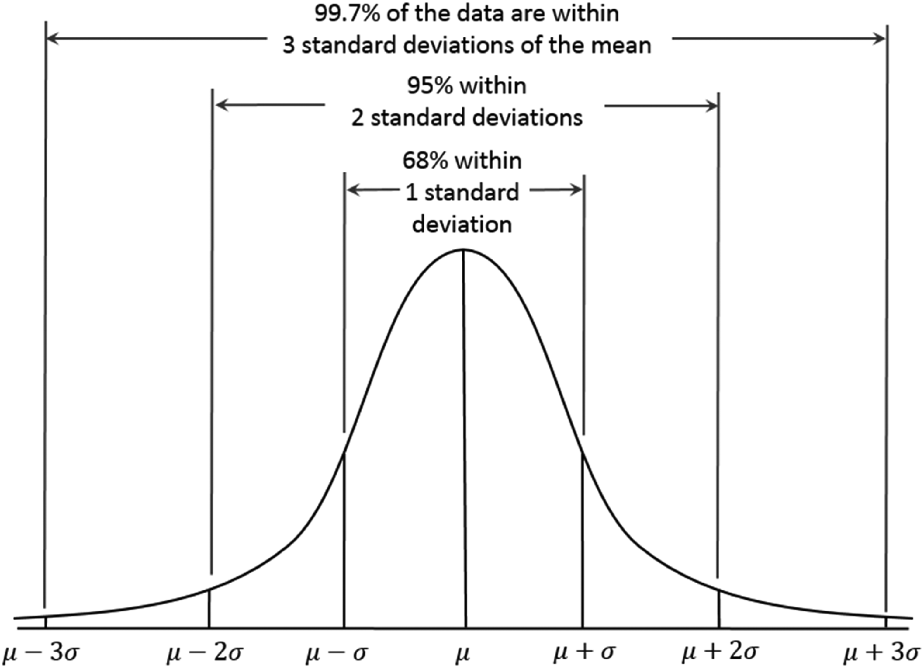
Gauss Random Variable. Source: Dan Kernler—Own Work, CC BY-SA 4.0, https://commons.wikimedia.org/w/index.php?curid=36506025

The Importance for Genealogy

How does any of this apply to genealogy? That is easy: other than height, many variables are actually random normal variables (or, more accurately, variables generated by a stochastic process that tends to distribute them as random casual variables, as suggested by the central limit theorem). Some of these variables are of genealogical interest, such as the lifespans of ancestors of interest.

It is common for a genealogist undertaking archival research to know the birth date of a subject of genealogical interest, but not the death date. The distance in years between the (known) birth act and the (desired) death act is simply, as the central limit theorem suggests, a random normal variable. Indeed the length of anyone's life is the result of the length of our parents’ lives, of those of our grandparents, and of many random normal variables (such as eating habits, physical activity, the probability of having various accidents, and so on). ⁴ This means that, again according to the Central Limit theorem, the variable years of life is distributed as a random normal variable.

Why is this useful to us? Because it allows us to improve our predictive ability, or in other words the possibility of inferring and deducing how many years the person in question is likely to have lived.

Indeed, by knowing the average life expectancy (ALE) of a person as similar as possible to one's ancestor, it can be determined that the probability of finding the death act will be highest in the year equal to the birth year plus the years of life expectancy. It is in correspondence with this year that the value of the random normal variable year of life reaches its maximum frequency (the peak of the bell). We also know that the probability shrinks and will continue to shrink the further we move away from the mean value (with higher probabilities the closer one is to the mean, from both sides, and lower probabilities moving further away from the mean).

To summarize, the central limit theorem suggests that the maximum probability of finding the death act of a subject of interest, Pmax, will be in the optimal year y*. This gives us, in formal terms:

P max = y *

(1)

y * = y b + A L E

(2)

In that sense, since ALE is an estimate it will always be an approximation of the ALE of the subject of interest; this approximation will be better the more it is estimated on an archetype similar to the ancestor. For example, if we wanted to estimate the ALE of a male born in Naples in 1983, the ALE of Italians born in 1980 is not as good a basis for our estimation as the life expectancy of males born in Campania (the region of Napoli) in 1983. Of course, at the same time, the former is a better basis for estimations than the life expectancy of females born in 1959, say.

Another interesting finding suggested by the central limit theorem is that probability shrinks as we move away from the mean value in both directions: this means that the highest probability of finding the act, once the possibility that the death act is in year y* is proven untrue, will be equally probable in the years y* − 1 and y* + 1 (since these are the next values for which the frequency is higher, given the bell shape). Once this is also found to be untrue, the new higher probability will be in the years y* − 2 and y* + 2. In genealogical terms, this means that once y* is known, the genealogist should start looking for the relevant act in the records for that year; if the act is not there, he or she should look in the registers corresponding to one year before and one year after y*, then two years before and two years after, and so on until the act is found. In this way, we are maximizing the probability of finding the act, and at the same time minimizing the time needed to find it. Optimizing the time dedicated to genealogy, with the help of a statistical method, will allow us to find more acts in the same amount of time, and thus increase our productivity, or in other words the results of our research.

Please note that similar reasoning may be used to estimate the year of death, by means of year of marriage (and age of the bride or the groom). In this case, our y* will be equal to:

y * = y m + A L E

(3)

Before starting to apply this method concretely in field research, the only thing left to understand is how to estimate the ALE. So far, we have taken this information for granted, but this cannot always be assumed in actual research situations.

Before proceeding, please note that we can further generalize the results obtained so far. Indeed, other than finding death acts, this approach may be used for other variables of genealogical interest. The number of years spent in celibacy is a random normal variable (as the summation of many random normal variables: what could be more random than when one meets his or her other half?), and so is the number of years before becoming a parent. We may thus apply the same reasoning to find the marriage or birth act of our ancestors, by means of the birth year or marriage year, respectively.

We may estimate the year of the (first) wedding by means of the average age at the wedding (average marriage age, AMA) of people as anthropometrically close to our ancestor as possible. In that case, y* will be the year of marriage, and be equal to

y * = y b + A M A

(4)

y * = y m + A M A

(5)

Looking for ALE and AMA

As stated previously, the only things that remain to be determined before applying this method in practice are the ALE and the AMA of a subject as close as possible to our ancestor of interest. There are some data available for this purpose. These have been included in the FAIT, which includes all the necessary data in one simple and user-friendly instrument.

Since 1974, the Italian National Statistics Institute (ISTAT) has offered life expectancies calculated for each Italian province by gender and year. Life expectancy is computed by ISTAT ⁵ as follows:

e x = L x + L x + 1 + ⋯ + L ! − 1 I x

(6)

A 2007 paper by Emanuele Felice ⁶ (which sources its data in a working paper by Leandro Conte, Giuseppe Della Torre, and Michelangelo Vasta) provides data from 1871 to the start of the twenty-first century. This computes life expectancy with a logarithmic scale to avoid flattening. Formally, it is computed as

L o g ( V a l M a x − V a l M i n ) − L o g ( V a l M a x − x i ) L o g ( V a l M a x − V a l M i n )

(7)

A V M a t − A V M a t − 1 a t − a t − 1

(8)

Finally, life expectancies for Northern Italy (Piedmont, Lombardy, Veneto, Emilia, and Tuscany) from 1650 onwards have been calculated by Galloway, ⁷ who uses an inverted projection technique. These estimates must be taken with caution, but it is interesting to have the opportunity to go back so far, and to the best of our knowledge there are no better estimates.

Substantially this technique aims to reconstruct, from known data about the population, namely births, deaths, and annual migration, the life expectancy, and, in consequence, the original size of the population. These data, estimated for the five provinces in Central and Northern Italy named above, are extended in the FAIT to all Italian regions. This means that the quality of our ALE in that case is not exceptional, even if it is better than the ALE calculated for the entire world.

We thus have estimates of ALE with the best possible data (to the best of our knowledge) available today. The estimates are differentiated by genders from 1974 onwards (ISTAT data), although due to lack of data this is not possible any earlier. Finally, it is important to note that for Molise and Abruzzo the ALE is calculated as if these were a single region (as they were in the past, which is also how Felice computes his estimates). As already specified, before 1871 all the data are referred to a mean value calculated from the five provinces in Northern Italy and applied to all the regions. In appendix A there is a summary of the sources for these data.

The AMA, meanwhile, is computed from data found in Rettaroli ⁸ and Da Molin. ⁹ The former offers statistics about the mean age at first marriage for Italian men and women, from 1861 to 1901. It also includes the same data retrieved from various Italian parishes, in various different Italian regions (Piedmont, Lombardy, Veneto, Emilia Romagna, Tuscany, Abruzzo, Puglia, Basilicata, Campania, and Sicily).

Da Molin offers data about the average age at first marriage for males and females from several parishes in Basilicata, Calabria, Puglia, and Campania. ¹⁰ These data are computed by Da Molin using the Hajnal method. ¹¹ Using all these data, we obtained a substantial amount of data for several Italian regions, filling in the years for which data are lacking by computing the harmonic average, as in the previous instance.

In appendix B, there is a summary of the sources for these data.

The FAIT

The computation of the equation that calculates the optimal year y* (i.e., the year in which the search for the relevant act begins) is performed automatically by the instrument. By inserting the data of the archetype closest to the subject of the research, i.e., birth year, gender, and region of residence, the FAIT will compute y*. Launching the Excel file, retrievable from https://sites.google.com/view/faitgenealogy, the screen in Figure 2 will appear.

OPEN IN VIEWER

Figure 2.

Launching Screen of FAIT. Note. FAIT = Forecasting and Inference Tool.

By clicking on the FAIT_Tool button, a new window with four options will appear. This is shown in Figure 3, and represents the four estimations FAIT is able to provide so far. Please note that by clicking on the flag a different translation (in one of the four available languages) of the available estimations will be provided.

OPEN IN VIEWER

Figure 3.

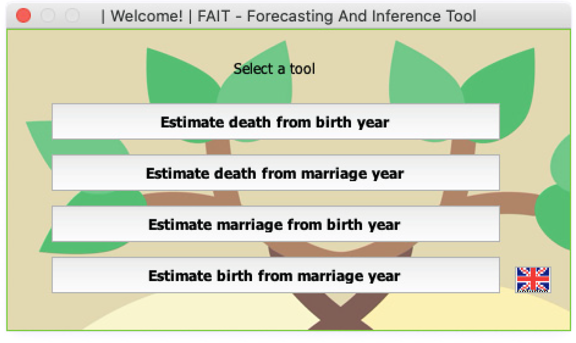
The Estimations Are Available on FAIT. Note. FAIT = Forecasting and Inference Tool.

These are estimation of the year of death from the birth year, estimation of the year of death from the marriage year, estimation of the year of marriage from the birth year, and estimation of the year of birth from the marriage year. These of course refer to the equation explained in section 4, with data presented in section 5.

Once the desired estimate has been selected, a new screen will appear. Figure 4 presents the screen for estimation of death from the birth year, although all four are very similar. In this screen, the user is required to provide the available information about the subject, such as year of birth (or of marriage, for estimations based on AMA), region of residence (since most of the data are heterogeneous for Italian regions), and gender (since the data differentiate between men and women). This enables the FAIT to find the ALE or AMA of a subject anthropometrically as close as possible to the subject being investigated.

OPEN IN VIEWER

Figure 4.

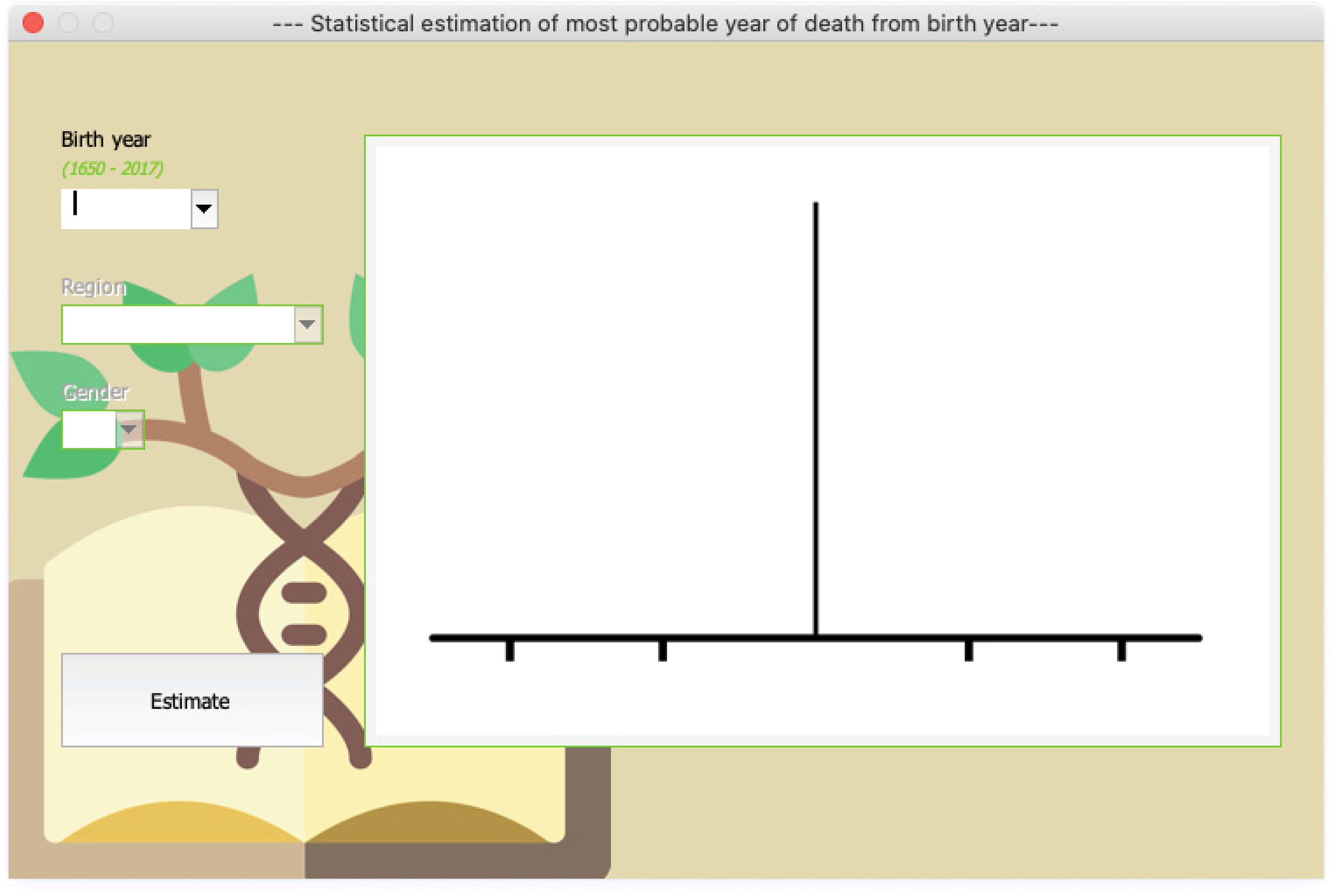
The Screen in Which Known Data May Be Inserted.

Once the required data are inserted, the tool proceeds to calculations, before displaying y*, i.e., the most likely year of death, marriage, or birth, and the year in which we should begin to search for the act we are interested in, in order to optimize the research.

For instance, in the example in Figure 5, the output is given for the estimate of the most likely year of death for a male that was born in Latium in 1877. As can be seen, the estimate is of 1909, and the probability of finding the act degrades to 0 as one heads towards 1877 or 1977.

OPEN IN VIEWER

Figure 5.

The Result of an Estimation of the Year of Death (by Means of the Birth Year).

Conclusions and Possible Future Expansions

In conclusion, we have presented some useful statistical applications for genealogy research. We have also introduced the FAIT, which we consider a very flexible instrument, and one that may in the future be further strengthened with new data, whether concerning Italy or other countries. Currently, it offers four different estimations, namely the estimation of the year of death from the birth year, the estimation of the year of death from the marriage year, the estimation of the year of marriage from the birth year, and the estimation of the year of birth from the marriage year.

Unfortunately, by its very nature this tool is highly dependent on the quality of available data; more studies in demography that help shed light on average ages in Italy or abroad would be needed to improve the ALE and AMA, and consequently the final estimate of y*.

In any event, we believe that a suboptimal estimate is better than no estimate at all and that the amount of data included in the tool (retrieved from the most up-to-date scientific literature available) exceeds what any genealogist can memorize and use proficiently in a given piece of research. Future updates may be focused on expanding the instrument's temporal and geographical scope by including data from other countries.