Quality-Differentiated Demand and the Analytics of Disruption

Abstract

The article builds on and extends two earlier teaching notes on the enhancement of undergraduate microeconomics to encompass quality considerations in consumer choice and market responses to those preferences. This enhanced framework is then applied to an analysis of market disruption, providing a credible and accessible path for predicting threats to higher end industry leaders from lower end competitors.

JEL Classifications: D0, D2, D4

Keywords

quality-differentiated demand market disrupt

Disruption from below is a well-known construct in business management studies. As Bower and Christensen (1995) note, “One of the most consistent patterns in business is the failure of leading companies to stay at the top of their industries when technologies or markets change” (p. 43). In retail markets, they give the example of Wal-Mart challenging Sears, that is, a stand-alone discount retailer newly emerging in the 1960s with an emphasis on lower prices challenging a long-established department store retailer with an emphasis on product line and differentiation and frequently anchoring shopping malls. A more recent example, particularly in rural areas, would be entrants such as “Dollar” stores challenging locally established IGA supermarkets and Five and Dime stores. More generally, Bower and Christensen note that, “[D]isruptive technologies introduce a very different package of attributes from the one mainstream customers historically value, and they often perform far worse along one or two dimensions that are particularly important to those customers” (p. 45).¹

The processes and dynamics of disruption examined by Bower and Christensen are based on empirical analyses and case studies with an emphasis on managerial incentives and decision-making. Approached deductively, the comparative statics of microeconomics would seemingly offer another useful perspective on disruption. In their article on digital disruption, Dawson et al. (2016) note that, “By subjecting the sources of disruption to systematic analysis solidly based on the fundamentals of supply and demand, executives can better understand the threats they confront in the digital space and search more proactively for their own opportunities” (p. 44).

Proceeding with a microeconomic analysis of how established firms controlling the higher end of the quality spectrum can be disrupted by new entrants operating at the lower end requires the ability to juxtapose quality-differentiated demand schedules. The objective of this article is to first elaborate on earlier efforts to derive such a demand structure and to then use it to predict how firms at the lower end affect production and pricing behavior at the higher end. This top-down approach to the analysis, predicated on gross assumptions of consumers maximizing utility and firms maximizing profits, is much different from the bottom-up case study approach underlying business management studies. But as a first approximation, it would appear that the two approaches complement each other in explaining and predicting disruptions to established firms.

Modeling Quality-Differentiated Demand

Previously in this Journal, a framework was presented for developing a quality-differentiated demand structure within the undergraduate microeconomics core (Adams, 2020). Most products have specific attributes that can be enhanced or degraded to create the possibility for higher and lower quality versions (e.g., reliability, freshness, and timely availability). The principle of vertical product differentiation dictates that the demand schedule for a higher quality version lies above that of a lower quality. Also, as previously argued, in a world of linear demand schedules, the simplest and most versatile configuration juxtaposing higher and lower quality demand schedules is one in which they are proportional to one another. Strict proportionality implies a constant marginal rate of substitution between higher and lower quality units of a quality-differentiated product and as Nutter (1955) notes, “[C]onstant marginal rate of substitution between products says nothing more than they are viewed as ‘perfect substitutes’ for each other” (p. 526). And with MRS_H,L = k > 1, the price consumers are willing to pay for higher quality units is everywhere k times the price they are willing to pay for lower quality units. Hence, taking the inverse of the lower and higher quality demand schedules, D_L and D_H, with P_L = a − bQ and P_H = k (a − bQ), D_H is proportional to D_L, with P_H = k P_L.²

As perfect substitutes, the optimal budget allocation for Q_H and Q_L is likely to culminate in a corner solution so that for any price ratio with P_H / P_L > k, the consumer chooses only lower quality units and vice versa for P_H / P_L < k. In effect, except for the special case where P_H / P_L = k, individual consumer demand for the quality-differentiated good manifests itself either in the market for higher quality units or the market for lower quality units, depending on relative prices.

It should be noted, too, that there are no income or substitution effects from changes in the price of one quality level to cause shifts in demand for the other quality level (Phlips, 1964). Such shifts would contradict the intrinsic relationship of the two goods as perfect substitutes governed by a constant marginal rate of substitution. Hence for P_H < kP_L, the consumer opts for all higher quality units and operates only along the higher quality demand schedule, D_H. With a reduction in P_H, there is no upward shift in D_L that would otherwise be expected from a positive income effect; as long as P_H is less than kP_L, demand for lower quality units remains at zero. Nor is there a negative substitution effect to cause a downward shift in D_L; with the initial demand for lower quality units at zero, it is not possible to substitute additional higher quality units for fewer lower quality units. However, once relative prices change so that P_H > kP_L, the consumer switches to the lower quality demand schedule and consumes only lower quality units.³ Hence, the a priori juxtaposition of D_H and D_L holds, with strict proportionality maintained between the quality-differentiated demand schedules.

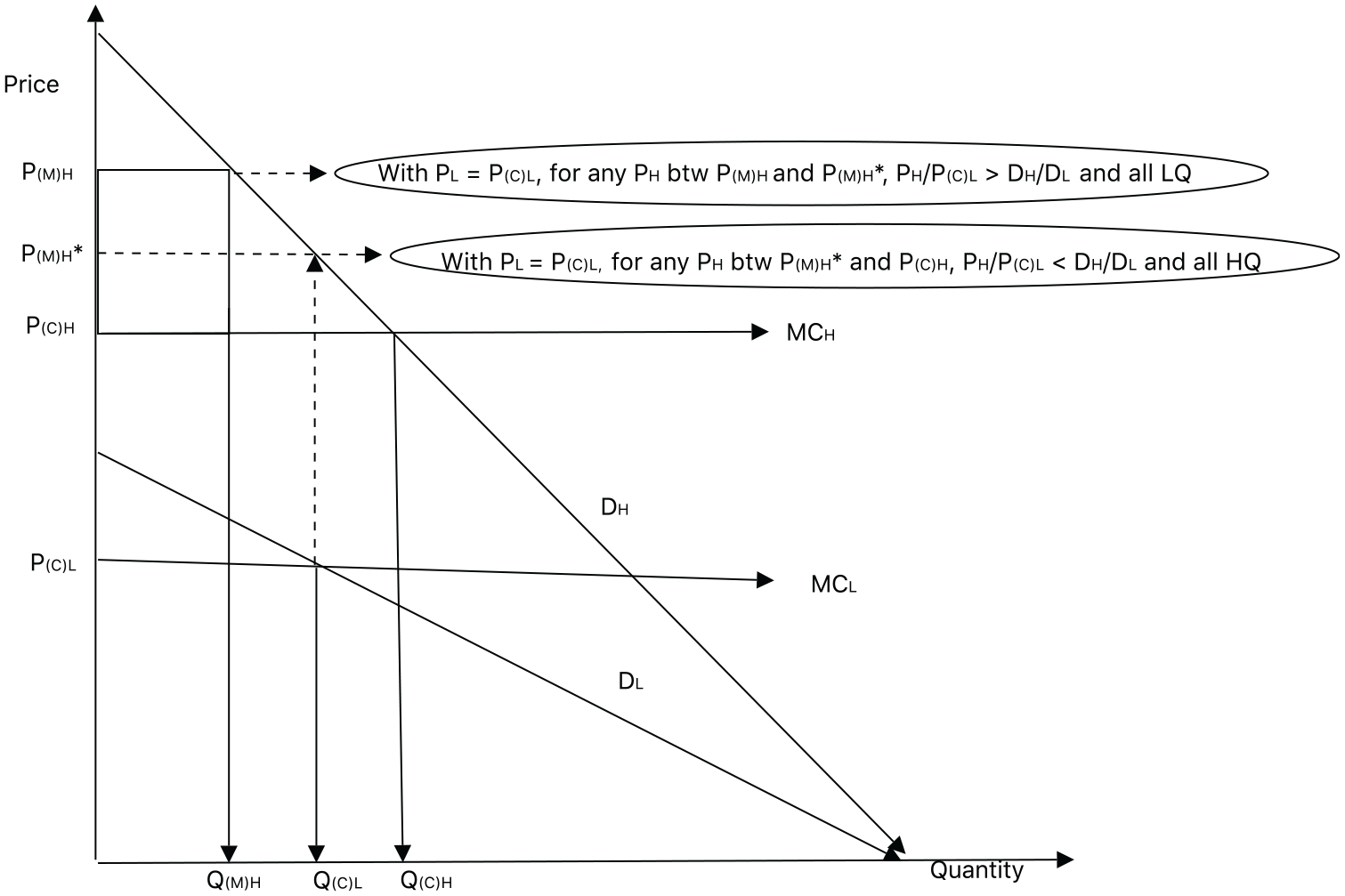
Such an arrangement is illustrated in Figure 1. D_H and D_L represent demand for higher and lower quality versions of the quality-differentiated product. D_H is everywhere 2 times the D_L which implies MRS_H,L = 2.⁴ Hence, for a price ratio P_H / P_L > 2, a corner solution obtains and the consumer chooses all lower quality units, and for P_H / P_L < 2, all higher quality units.

Figure 1.

Consumers optimize by choosing only higher quality.

Potential competitive market equilibria occur in Figure 1 at the intersection of each demand schedule and its corresponding MC schedule.⁵ MC_H and MC_L represent long-run marginal cost schedules under the assumption of constant cost industries, with MC increasing as quality increases. Using Q_(C)H as a reference point, it can be seen that with marginal cost pricing, P_(C)H / P_(C)L is less than D_H / D_L. Hence, the optimal quality choice for consumers is all higher quality.

A similar result obtains in the monopoly case. Assume for the moment that a single firm controls production of both the higher and lower quality versions of the quality-differentiated good. Using Q_(M)H as a reference point, P_(M)H / P_(M)L is less than D_H / D_L and consumers optimize by choosing only the higher quality. Moreover, the monopolist maximizes profit by selling only the higher quality version. Both sales volume (Q_(M)H) and per unit profit margin (P_(M)H − MC_H) clearly exceed the lower quality version with potential profits over 3 times those of the lower quality.⁶ The monopolist establishes a profit-maximizing and stable equilibrium by producing and selling only the higher quality version of the product. Its control over the lower quality version notwithstanding, any move toward selling at the lower end would result in reduced profit.

Analytics of Disruption

Applied to the analysis of Bower and Christensen, our monopolist takes on the role of an established industry leader at the higher end of the quality spectrum.⁷ Moreover, were a market to develop at the lower end, the authors argue that a common propensity is for our industry leader to stay narrowly focused on better servicing its higher end customer base and to ignore developments at the lower end of the industry.

[T]he processes and incentives that companies use to keep focused on their main customers work so well that they blind those companies to important new technologies in emerging markets. Many companies have learned the hard way the perils of ignoring new technologies that do not initially meet the needs of mainstream customers. For example, although personal computers did not meet the requirements of mainstream minicomputer users in the early 1980s, the computing power of the desktop machines improved at a much faster rate than minicomputer users’ demands for computing power did. As a result, personal computers caught up with the computing needs of many of the customers of Wang, Prime, Nixdorf, Data General, and Digital Equipment. Today they are performance-competitive with minicomputers in many applications. For the minicomputer makers, keeping close to mainstream customers and ignoring what were initially low-performance desktop technologies used by seemingly insignificant customers in emerging markets was a rational decision—but one that proved disastrous. (Bower & Christensen, 1995, p. 44)

Referring back to Figure 1, assume that a lower end market evolves as a competitive market. Once these lower end firms emerge, the established higher end firm confronts an untenable situation. The lower end competitive market operates according to marginal cost pricing and establishes a price of P_(C)L for the lower quality product. The dominant firm at the high end continues to seek maximum profit at P_(M)H − Q_(M)H, but this is no longer a sustainable equilibrium. By inspection, P_(M)H / P_(C)L > 2. Hence, our utility maximizing consumers in Figure 1 switch from the higher to the lower end of the market.⁸

Facing the virtual collapse of its higher quality market, the established firm only survives if it lowers its price to the point where P_H / P_L falls below 2. In Figure 2, this occurs once the firm lowers its price to just below P_(M)H*, increasing the output of the higher quality version to a level greater than Q_(C)L. Once established, this new equilibrium is stable; lower end sellers, unable to respond by lowering their prices without incurring economic losses, must be satisfied with any new and emerging market for their lower quality units, one independent of the dominant firm’s established customer base. The firm’s profit margin is reduced, and production of the higher end version increases and moves closer to the socially efficient rate, Q_(C)H. This makes up more than half of the socially suboptimal rate of production at the higher end.

Figure 2.

Disruption from below.

Limits to Disruption

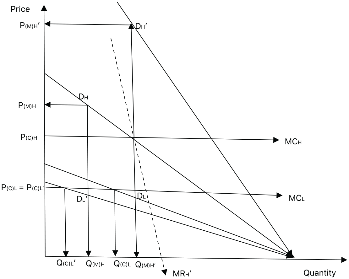
While a microeconomics analysis predicated on a quality-differentiated demand structure provides a useful point of departure for predicting how lower end markets can disrupt established higher end markets, it is also instructive about the limits to such disruption. These limits are illustrated in Figure 3 which extends the initial demand structure in Figures 1 and 2. First, if higher end demand is sufficiently strong as reflected in the demand schedule D_H’, the monopolist’s higher end equilibrium, Q_(M)H’, will be established at a price, P_(M)H’, such that P_(M)H’ / P_(C)L is less than D_H’ / D_L. Consumers, therefore, optimize by purchasing only the higher quality product and the dominant firm establishes a sustainable profit-maximizing equilibrium for its higher end product, the emergence of a lower end competitive market notwithstanding.

Figure 3.

Limits of disruption.

Alternatively, if the lower end demand in the market served by the monopolist is sufficiently weak as reflected in the demand schedule D_L’, the monopolist’s initial higher end equilibrium, P_(M)H − Q_(M)H, is such that P_(M)H / P_(C)L’ is less than D_H / D_L’. Again, its customers optimize by purchasing only the higher quality product and the dominant firm establishes a sustainable profit-maximizing equilibrium unaffected by the emergence of the lower end competitive market.⁹

Hence, operating within the comparative statics of microeconomics, threats from below to an established high-end firm will depend on the particular quality-differentiated demand structure it operates in. Subsequent developments and structural shifts such as those described by Bower and Christensen with established industry leaders repeatedly failing to appreciate threats from below and the formation of new markets and technological advances by lower end entrants cannot be deduced from the microeconomics but require more qualitative, on-the-ground case study.

Conclusion

This exploratory analysis, predicated on quality-related aspects of market dynamics, can open up in a variety of ways to allow for heterogeneous consumers, multiple uses of a quality-differentiated product, and a variety of market structures and public policy considerations. The specific focus of this article has been on how such a framework can be applied to the analytics of market disruption. Threats to established firms from lower end industry entrants are a predictable threat. Short-term profit-maximizing pricing and output behavior governing the higher end of the quality spectrum may not be sustainable if the established firm fails to exert control over the lower end as well. As a corollary, those responsible for regulating and limiting monopoly abuses may find an effective and easier path by ensuring competitive practices and conditions among smaller, more disparate entrant firms than in countering rent-seeking behaviors by established firms with greater concentrated power.

Footnotes

Appendix

A utility structure predicated on the assumption of a constant MRS between higher and lower quality units of a quality-differentiated good can be adapted from one used by Deaton and Muelbauer (1980, p. 262). Assuming a single quality-differentiated good, Q₁, with two quality levels—higher quality units $Q_{1}^{H}$ and lower quality units $Q_{1}^{L}$ —such a structure would incorporate a subutility function, $V = V (α Q_{1}^{H} + β Q_{1}^{L})$ with α > β and reflecting a constant MRS and perfect substitution between $Q_{1}^{H}$ and $Q_{1}^{L}$ and less-than-perfect substitution between each of them and all other goods, Q₂, . . .,Q_N, that is, $U = U (V (α Q_{1}^{H} + β Q_{1}^{L}), Q_{2}, \dots, Q_{N})$ . Underlying this utility structure is the assumption of weak separability, with choices about the mix of Q₁ quality levels independent of choices about all other goods, Q₂ . . . Q_N. Hence, the assumption of a constant MRS between higher and lower quality units of the quality-differentiated good holds, regardless of the choices made about all other goods.

Given income, Y, prices for the higher and lower quality units of the quality-differentiated good, $P_{1}^{H}$ and $P_{1}^{L}$ , and prices for all other goods, P₂, . . ., P_N, an optimal budget allocation can be derived by setting up the Lagrangian and solving for pertinent first-order conditions as follows:

(1)

L = U {V (α Q_{1}^{H} + β Q_{1}^{L}), Q_{2}, \dots, Q_{N}} + λ (Y - P_{1}^{H} Q_{1}^{H} - P_{1}^{L} Q_{1}^{L} - P_{2} Q_{2} - \dots - P_{N} Q_{N}),

(2)

\frac{δ L}{δ Q_{1}^{H}} = \frac{δ U}{δ V} α - λ P_{1}^{H} = 0,

(3)

\frac{δ L}{δ Q_{1}^{L}} = \frac{δ U}{δ V} β - λ P_{1}^{L} = 0,

(4)

\frac{δ L}{δ λ} = Y - P_{1}^{H} Q_{1}^{H} - P_{1}^{L} Q_{1}^{L} - P_{2} Q_{2} - \dots - P_{N} Q_{N} = 0 .

From Equation (4), the demand schedule for higher quality units can be expressed as follows:

(5)

Q_{1}^{H} = \frac{(Y - P_{1}^{L} Q_{1}^{L} - P_{2} Q_{2} - \dots - P_{N} Q_{N})}{P_{1}^{H}} .

Solving for P^H₁ in Equation (2) and substituting in Equation (5) yields the following:

(6)

Q_{1}^{H} = \frac{(Y - P_{1}^{L} Q_{1}^{L} - P_{2} Q_{2} - \dots - P_{N} Q_{N})}{(δ U / δ V α / λ)} .

Similarly, the demand schedule for lower quality units is as follows:

(7)

Q_{1}^{L} = \frac{(Y - P_{1}^{H} Q_{1}^{H} - P_{2} Q_{2} - \dots - P_{N} Q_{N})}{(δ U / δ V β / λ)} .

Dividing Equation (6) by Equation (7) yields the following:

(8)

\frac{Q_{1}^{H}}{Q_{1}^{L}} = (\frac{β}{α}) (\frac{P_{1}^{H} Q_{1}^{H}}{P_{1}^{L} Q_{1}^{L}}) .

Setting $Q_{1}^{H}$ = $Q_{1}^{L}$ and solving for $P_{1}^{H}$ yields the following:

(9)

P_{1}^{H} = (α / β) P_{1}^{L} = k P_{1}^{L} with k > 1 .

Hence, as presented in the text, prospective demand schedules for higher and lower quality units of a quality-differentiated good are strictly proportional to one another.

At each quantity, the price the consumer is willing to pay for higher quality units is k times the price he is willing to pay for lower quality units. As consumption of higher (or lower) quality units increases, his willingness to substitute higher (or lower) quality units for all other goods decreases along with the price he is willing to pay for those units. But his willingness to substitute higher for lower quality units is unchanged and the relative price he is willing to pay for higher quality units remains constant at k times the price he is willing to pay for lower quality units.

Acknowledgments

The author wishes to thank Professor Paul Grimes, Editor-in-Chief of the American Economist, as well as various anonymous reviewers and associate editors for helpful comments on this and two earlier teaching notes on quality-differentiated demand.

Declaration of Conflicting Interests

The author(s) declared no potential conflicts of interest with respect to the research, authorship, and/or publication of this article.

Funding

The author(s) received no financial support for the research, authorship, and/or publication of this article.

ORCID iD

Charles F. Adams

Notes

Author Biography

Charles F. Adams is Professor Emeritus, John Glenn College of Public Affairs, Ohio State University.

References

Adams

C. F.

(2015). Quality-differentiated demand and market efficiency. https://papers.ssrn.com/sol3/papers.cfm?abstract_id=2576773

Adams

C. F.

(2020). An undergraduate primer on quality-differentiated demand. The American Economist, 65(2), 277–283.

Akerlof

G. A.

(1970). The market for lemons. Quarterly Journal of Economics, 84(3), 488–500.

Bower

J. L.

Christensen

C. M.

(1995). Disruptive technologies: Catching the wave. Harvard Business Review, 73(1), 43–53.

Dawson

Hirt

Scanlon

(2016). The economic essentials of digital strategy. McKinsey Quarterly, Issue 2, Article 32.

Deaton

Muelbauer

(1980). Economics of consumer behavior. Cambridge University Press.

Meyershon

(2019, July 19). Dollar stores are everywhere: That’s a problem for poor Americans. CNN Business.

Nutter

G. W.

(1955). The plateau demand curve and utility theory. Journal of Political Economy, 63(6), 525–528.

Phlips

(1964). Demand curves and product differentiation. Kyklos, 17(3), 404–418.

10.

Rosen

Rosenfield

A. M.

(1997). Ticket pricing. The Journal of Law and Economics, 40(2), 351–376.

11.

Tirole

(1988). The theory of industrial organisation. The MIT Press.