



Abstract
The spatial elements of crime occurrence and the identification of crime generators/attractors have remained a prominent area of research. We focus on the utility of the 80-20 rule and the labeling of risky facilities in crime forecasting models with risk terrain modeling (RTM). We first examine whether the rule holds across types of crime generating places including liquor stores, department stores, hotels/motels, restaurants/bars, and apartment complexes. Next, we use our findings to test whether conducting preliminary analyses to identify risky facilities increases the predictive power of RTM versus using all possible facilities. When restricting the RTM approach to only risky facilities, results were more accurate than a traditional RTM approach. Findings and implications are nested in the utilization of the wider body of environmental criminology research to increase our understanding of where crime is likely to occur.
Keywords
Traditionally, research has overwhelmingly focused on understanding who commits a crime, leading to the identification of chronic offending by Wolfgang and colleagues. Their landmark finding was that 6.3% of delinquent youth accounted for 52% of the recorded police contact. In other words, most youths are not delinquent, but a subset of youth is best described as chronic offenders. More contemporary research continues to support this general finding that a small percentage of individuals account for a disproportionate amount of any particular crime outcome (e.g., Vaughn & DeLisi, 2008). Although there are relatively few chronic offenders, considerable attention is afforded to those offenders due to the disproportionate amount of crime that is attributed to them (McGloin & Stickle, 2011). With a focus on who commits the crime, where crime occurs warrants the same focus. Certainly, research continues to indicate crime is not random in space and time, leading to a small percentage of places accounting for a disproportionate share of crime occurrence.
As a growing analytical tool, risk terrain modeling (RTM) has been utilized to identify attributes from the environment spatially associated with crime occurrence (RTM; see Caplan et al., 2011; Caplan & Kennedy, 2016; Kennedy et al., 2018). RTM has a foundation in environmental criminology, focusing primarily on the spatial attributes of crime with temporal scales of secondary priority, including the influence of crime generators and attractors (CGAs; see Brantingham & Brantingham, 1995). These features of the environment such as bars, restaurants, rental housing units, public transit stops, and so on, attract or generate crime based on their presence. Yet while advancements in RTM applications have furthered crime and place research, the risk terrain approach overlooks variability in crime occurrence at any one facility type. That is, RTM can identify bars as crime risk generators or attractors, but ignores important issues raised by environmental criminology broadly, and the “80-20 rule” specifically (Clarke & Eck, 2003; Eck et al., 2007). In short, and expanded on later, the 80-20 rule stipulates that a small subset of establishments of one type of facility (20%) usually accounts for a majority of crime (80%), identifying certain risky facilities.
The current study builds on these observations to test the predictive accuracy of RTM using a model limited to only risky facilities. To do so, we compare risk terrain models for all facilities against a risky facility model using two crime types—aggravated assaults and theft from a motor vehicle—for the calendar year 2018 to forecast January through September 2019 crime occurrence in Little Rock, AR. These models are compared using the updated predictive accuracy index (PAI) outlined by Drawve and Wooditch (2019), building from Chainey et al.’s (2008) original metric. In addition, we compare the predictive accuracy of the two RTM analyses to a more simplistic approach, risky facility buffers.
Review of Literature
Extant literature dating back to Guerry (1833) and Quetelet (1831) demonstrate spatial patterning in crime occurrence. Subsequently, Sherman et al. (1989) brought this argument to prominence in more contemporary research at the microlevel with emphasis on the hotspots of crime. In comparison to studies of individual criminal offending, spatial research has found that the concentration of crime within relatively few places is more extreme than the disproportionate offending of high-crime individuals (Spelman & Eck, 1989). Naturally, research has sought to leverage theory to understand why crime occurs in specific places, including through the lenses of routine activities theory (Cohen & Felson, 1979) and crime pattern theory (P. J. Brantingham & Brantingham, 1984) leading to the development of the law of crime concentration (Weisburd, 2015). In turn, this has led to an increased effort to forecast where crime is going to occur, often down to the street level, in hopes of being able to implement place-based efforts to reduce offending or prevent crime from occurring at all.
Environmental Criminology Foundation
Environmental criminology often relies on three theoretical perspectives as the foundation to explain why crime occurs in specific spaces at particular times: routine activities theory, rational choice theory, and crime pattern theory. Routine activities theory argues criminal opportunities are present during daily routine activities such as going to school, work, and running errands when a likely target, motivated offender, and lack or absence of capable guardianship converge in time and space. When multiple people have similar or overlapping routine activities, this leads to the concentrations of criminal opportunities at certain places. Although there are opportunities for crime, offenders still have to make the decision to act. Presented with criminal opportunities, the decision to act follows a rational choice model where the offender seeks to maximize their rewards while minimizing the risks involved (see Cornish & Clarke, 1986). Brantingham and Brantingham (1995) use the elements of routine activity theory to build onto the offender’s decision-making process within the environment through crime pattern theory.
Crime pattern theory (P. J. Brantingham & Brantingham, 1984, 1993) extends these propositions with the introduction of spatial concepts, including nodes, paths, and edges, that lead to people developing an awareness of their surrounding environment. It is within offenders’ “awareness space” that criminal opportunities are identified. Thus, people spend time in major nodes (e.g., home, work) and travel to and from them along paths bound by physical (e.g., river) and social edges, representing the larger environmental backcloth. Germane to the current study, Brantingham and Brantingham (1995) highlighted the influence of CGAs. While the two concepts are similar in nature, crime generators draw people to a location for noncriminal purposes, but criminal opportunities arise based on the convergence of victims and offenders. In contrast, crime attractors draw motivated offenders to their locations based on likely targets that lack capable guardianship. Extant literature finds a number of different CGAs such as liquor stores (Block & Block, 1995), bars (Groff, 2011; Ratcliffe, 2012), fast-food restaurants (P. J. Brantingham & Brantingham, 1984), public transit (Hart & Miethe, 2014), stadiums (Kurland et al., 2014), and parks (Groff & McCord, 2012) to be associated with crime occurrence. The focus on such places has led to a parallel line of research examining the spatial distribution of crime, known as the law of crime concentration.
Weisburd’s (2015) Sutherland lecture spurred a growing contemporary literature on the concentration of crime. In the simplest forms, and without delving into the ways to measure concentration, when studying the spatial distribution of crime, a majority percentage of crime occurs within a small percentage of places, resulting in a concentration. Research supports the underlying argument of the law of crime concentration across suburban settings (Gill et al., 2017), temporal scales (Haberman et al., 2017; Levin et al., 2017), international settings (Favarin, 2018), and with updated reporting methodology (Bernasco & Steenbeek, 2017). While this body of literature has, and will continue, to expand crime and place approaches, there is a specific focus on the concentration of crime with little attention directed toward what contributes to the crime occurrence. This gap, and more broadly from hotspot-specific literature, led to the development of a spatial analytical approach known as RTM.
RTM is a spatial analytical tool that combines concepts from environmental criminology and spatial analysis for studying spatial vulnerability to crime (Caplan & Kennedy, 2016). RTM examines how different types of CGAs (e.g., bars, liquor stores, bus stops, parks, and ATMs) combine together to create a risk profile for different crime types across space. That is, we might know both bars and liquor stores influence crime, but when in close proximity to one another, the risk might be even greater, perhaps exponentially, for crime to occur. Prior research has demonstrated the utility of RTM to identifying significant CGAs for a variety of offenses including child maltreatment (Daley et al., 2016), drug dealing (Barnum et al., 2017), aggravated assault (Thomas & Drawve, 2018), gang violence (Valasik, 2018), homeless crimes (Yoo & Wheeler, 2019), robbery (Feng et al., 2019), suicide attempts (Lersch, 2020), opioid overdoses (Chichester et al., 2020), property crime (Andresen & Hodgkinson, 2018; Piza et al., 2017), and terrorism (Marchment et al., 2019). These analyses typically focus on place-based approaches to how prevention resources could be efficiently and effectively allocated based on the underlying diagnostics conducted by RTM.
L. W. Kennedy and Caplan (2013) proposed a theory of risky places outlining how vulnerability and exposure led to crime occurrence. In short, the theory of risky places argues that (a) all places are at risk of crime but that features from the environment (e.g., CGAs) combine to create some places that are much riskier than others. By extension, (b) crime occurs where vulnerability is high because multiple CGAs independently influence crime occurrence, creating an additive vulnerability, which in turn means (c) the effect risky places have on crime depends on both vulnerability and exposure (see L. W. Kennedy et al., 2016). This leads to how features from the physical environment—bars, bus stops, liquor stores, pawnshops, and so on—create vulnerable places for crime, particularly when they coexist. At the same time, however, prior exposure to crime matters at those highly vulnerable places since crime would not be as likely to occur there in the future without it. Within the current RTM approach (see below), researchers typically account for crime exposure by combining RTM results with other analytic techniques, such as hotspots and near repeat analyses (e.g., Caplan et al., 2013; Drawve et al., 2019). This step in controlling for exposure is usually completed after generating the RTM results rather than developing preliminary steps to account for exposure, as outlined in the current study.
Unfortunately, the focus on vulnerability within RTM approaches has overlooked prior work identifying risky facilities. Specifically, the current application of RTM assumes homogeneity in risk across CGA type (bar, park, liquor store, school, etc.). As an example, RTM could identify fast-food restaurants as risky, but the underlying assumption is that all fast-food restaurants are equally risky for crime. Critically, such an assumption overlooks broader environmental criminology concepts related to the distribution of crime at CGAs: Crime is not random as evidenced by “the fact of hot spots” (see P. J. Brantingham et al., 2020, p. 61), so not every facility of a specific type (e.g., fast-food restaurants) is likely to be uniformly risky.
Risky Facilities and the 80-20 Rule
That some risky facilities are riskier than others remains an important observation from environmental criminology. As Eck et al. (2007, p. 226) state, “…for any group of similar facilities (e.g., taverns, parking lots, or bus shelters), a small proportion of the group accounts for the majority of crime experienced by the entire group.” Thus, not all facilities of one type are equally associated with criminal offending, resulting in risk heterogeneity within a facility type. Within the extant criminology and criminal justice literature, this is known as the “80-20 rule” (see Clarke & Eck, 2007), though other fields refer to this as the Pareto principle. In short, the 80-20 distribution proposes that a minority of causes, inputs, or effort usually lead to many of the results, outputs, or rewards (Koch, 2003). Within the distribution of a facility type (or CGA), the distribution of crime across those types of facilities follows a J curve with a smaller percentage of facilities accounting for the majority of crime (see Blair et al., 2017). This observation has led to the proposed Iron Law of Troublesome Places (see Wilcox & Eck, 2011) and found support across the literature on risky facilities and the 80-20 rule (e.g., Blair et al., 2017; Bowers, 2014; Groff & McCord, 2012; Townsley et al., 2014). Just as Wolfgang et al. (1972) identified that a relatively small number of chronic offenders are responsible for a disproportionate amount of crime, we can expect roughly 20% of facilities to be linked to approximately 80% of offenses. This 20% of facilities are referred to as risky facilities.
Current Study
Although research supports the risky facility argument and the 80-20 rule more broadly, these concepts have largely been overlooked in much of the extant crime and place research, which has instead emphasized the ability to forecast crime as a priority. Thus, the current study seeks to take the somewhat forgotten risky facility argument and examine how that approach intersects with an RTM approach. To the researchers’ knowledge, this has not been conducted in prior RTM applications. We argue that, to better assist in crime forecasting, we must utilize a descriptive risky facility approach in order to identify the riskiest facilities within specific facility subtypes (apartment complexes, restaurants, liquor stores, hotels/motels, and department stores). It should be noted that there are analytical limitations when only relying on one tool in the toolbox, such as RTM. We seek to develop a modified approach, resulting in better usage of that analytical tool to understand crime occurrence in Little Rock, AR.
Data and Methodology
Little Rock, AR, is a strategic research site as the capital city and the most populated city in the state, holding a population of around 200,000 persons. Little Rock has population characteristics of 51% White and 42% Black, with 41% of the population holding a bachelor’s degree or higher and median household income around US$50,000 (below the U.S. median). Moreover, 17.4% of residents are in poverty (above the U.S. mean; census.gov). On top of that, Little Rock has continued to be a high crime city for both property and violent offenses, typically being in the top 10 cities with populations over 100,000 persons. In 2018, Little Rock had a violent crime rate of 1,449 per 100,000 compared to a national rate of about 381. Likewise, Little Rock’s property crime rate of 6,575 per 100,000 far exceeds the rate of about 2,200 for the nation as a whole (crimedatatool.com). Additionally, we use Little Rock as our study site, given the prior RTM-related work conducted on the city (e.g., Chillar & Drawve, 2018; Drawve & Barnum, 2017; Drawve et al., 2016; Thomas & Drawve, 2018).
Data for the current study came from the city of Little Rock. The researcher(s) have an existing memorandum of understanding for data sharing between city agencies and researcher(s), allowing us to obtain data for the current study in a timely manner. Crime data were provided by a crime analyst with the Little Rock Police Department (LRPD) for 2018 and part of 2019 crime incident reports (National Incident Based Reporting System (NIBRS); i.e., crime reported to police). Specifically, we focus on two different crime types, aggravated assault and theft from motor vehicles. For 2018, Little Rock had 2,247 aggravated assaults and 9,879 thefts from motor vehicles. The 2018 data were used to identify risky facilities and January to September 2019 were used for forecasting, allowing for comparisons between approaches. These are two separate analyses to increase the robustness of findings.
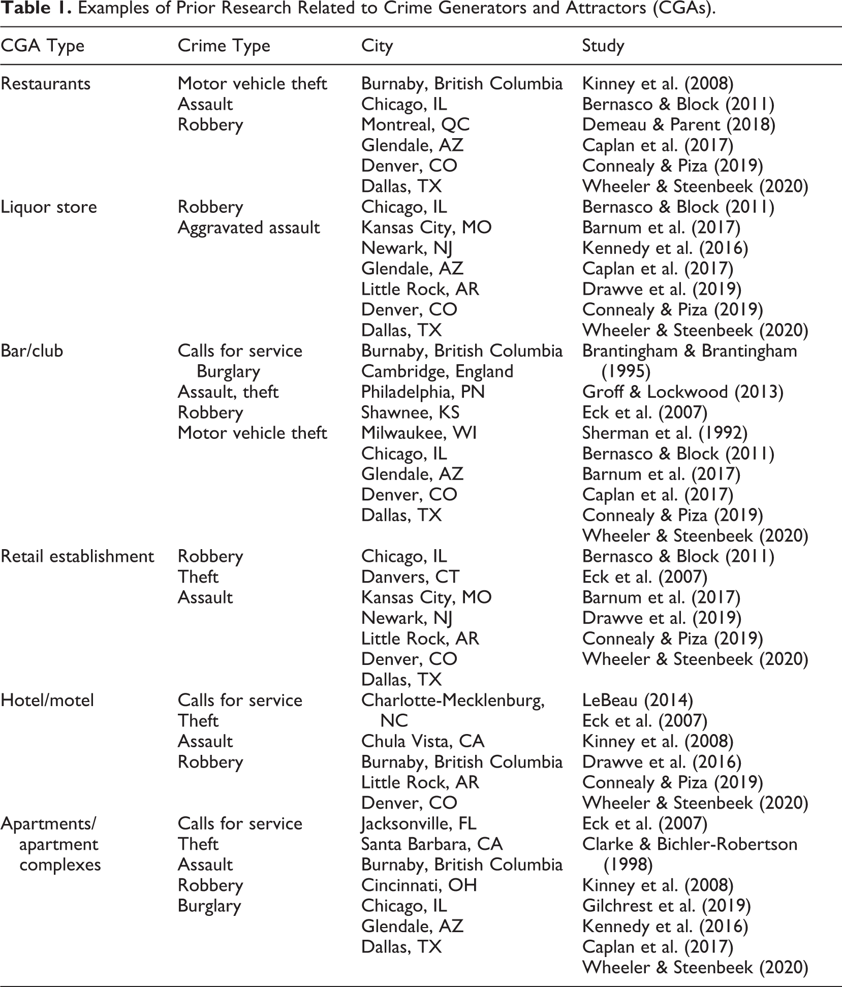
To gather data on potential CGAs and to identify risky facilities, we obtained a data set of businesses operating in Little Rock from the city’s treasury department. Our CGA classification is, therefore, based on how the city categorizes businesses, trying to keep in line with how practitioners record and use data internally to city operations. We focus our analyses on a subset of CGAs: apartment complexes (n = 350), liquor stores (n = 55), hotels/motels (n = 69), bars/restaurants (n = 231), and major chain department stores (n = 15). 1 We focused on this subset of CGAs, given their significance in prior Little Rock–specific RTM research (Chillar & Drawve, 2018; Drawve & Barnum, 2017; Drawve et al., 2016; Thomas & Drawve, 2018). Broadly, these facilities are chosen and categorized because they are theoretically most vulnerable to crime because of the confluence of motivated offenders and suitable targets in time and space either by “generating” criminal opportunities (e.g., bars, apartment complexes) or “attracting” them (e.g., parks, hotels/motels). Beyond Little Rock–specific work, Table 1 outlines the larger literature focusing on these risk factors and their relationship with crime. We acknowledge here and later that the current selection of CGAs should be expanded on in future approaches.
Examples of Prior Research Related to Crime Generators and Attractors (CGAs).
Analytical Framework
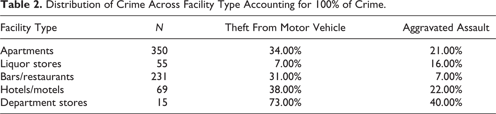
The first step in our study is to identify the risky facilities for each crime type, aggravated assault, and theft from a motor vehicle. Since the crime and CGA data are address level, we are able to identify the distribution of crime across each facility type. We compare exact addresses with no buffer around a facility for this step. An issue emerges with specific facilities having the same count of crime, meaning that there would have to be an arbitrary cutoff for a number of facilities accounting for 80% of crime. That is, a facility type could have numerous facilities having two crimes occurring at their location, taking the total percentage of crime past 80%; however, excluding a particular facility would not be appropriate since multiple facilities have the same number of crimes. To avoid these arbitrary cutoffs and for the 80-20 framework, we include all facilities with the same count of crime. This results in a smaller proportion of facilities across each type accounting for 100% of each crime, as seen in Table 2. Table 2 shows the percentage of each facility type accounting for 100% of each crime at those facilities. For example, Table 2 shows that 34% of all apartment complexes account for all theft from a motor vehicle that occurs at apartment complexes, while 16% of liquor stories account for all aggravated assault that occurs at liquor stores.
Distribution of Crime Across Facility Type Accounting for 100% of Crime.
Next, the risky facilities are used within RTMDx (Caplan & Kennedy, 2018), a software developed to automate the risk terrain process. In brief, RTMDx requires the user to set parameters before testing, including:
Study area: set to Little Rock boundary (municipal shapefile);
Model type: set to aggravating rather than protective, meaning that we assume the risk factors correlate with the location of the crime and then test for a positive relationship;
Unit of measurement standard value: set to 414 ft based on the average block length in Little Rock with a place size half, that is, 207 ft. Prior research has suggested that block length is a more realistic unit for agencies and that crime-ridden places consist of few street blocks (Kennedy et al., 2011; Taylor, 1988; Taylor & Harrell, 1996);
Analysis issue: set to 2018 aggravated assault or 2018 theft from a motor vehicle, respectively (point shapefiles); and
Input of risk factors: loaded each facility type separately then specified: Operationalization: set to both proximity and density. This allows for RTMDx to test whether being in close proximity to a facility is risky itself or if a place is risky based on the density (clustering) of a facility type, Standard value multiplier: set to four. Since our stand value was set to 414 ft above, this would result in RTMDx testing for a relationship up to four blocks, and Analysis increments: set to half, which means RTMDx will test the spatial relationship at half-block increments (207 ft) up to four blocks (standard value multiplier).
The risk factor process results in numerous variables being created for one CGA. For example, within the full model, apartment complexes were set to both (proximity and density), with a standard multiplier of four, and analysis increment set to half. This would result in eight proximity variables (half block up to four blocks) and eight density variables for apartment complexes alone to test the relationship between their locations and crime. This is a benefit of the automation process within RTMDx.
In short, RTM uses a two-step approach to build the “best” fitting model. The first step is to select risk factors that are significantly related to the outcome event. This step excludes variables that are not significantly related to the outcome event, in our case, aggravated assault or theft from motor vehicles, respectively. The second step is a bidirectional stepwise regression to improve model fit based on the Bayesian information criterion score. The “best” fitting model is then retested using both Poisson distribution and a negative binomial distribution to finalize that “best” model (for greater details on the RTM process and statistical approach see Caplan & Kennedy, 2016, and Garnier et al., 2018). The final output indicates significant risk factors, their respective operationalizations, and risk values along with a risk terrain map. In other words, RTM creates a model that identifies the most appropriate risk factors for the outcome variable (Caplan & Kennedy, 2014). Each factor is given a relative risk value that is the weight of the risk factor that can be compared across factors. The RTMDx output is in grid cells, similar to a fishnet over a study area, with each cell having an assigned relative risk score (see Figure 1 for visualization). Since risk cells are generated for the entire study area of Little Rock, cells intersecting streets were used to identify high-risk streets (discussed further below). This process was also conducted with the full list of CGA facilities that we can use to compare predictive accuracy across models.

Illustration of risk layering over a study area.
To compare risky facility RTMs to all facility RTMs, we use the modified PAI discussed by Drawve and Wooditch (2019). The formula is:
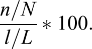
where n is the number of predicted crimes over the total crimes N in the numerator (hit rate), and the denominator is the length of streets within the predicted area (l) over the total length of streets in the study area (L). This results in a PAI value that is comparable across forecasting techniques, in our case, the risky facility RTMs to all facility RTMs. Additionally, given that both approaches are based on RTMDx, we explore the use of cells in the denominator (c/C), where c is the number of risky cells in which crime is expected to occur in the future over the total number of cells, C.
The 2018 risky facility RTMs and all facility RTMs are compared as they predict 2019 crime, respectively (January to September). Risky places expected to have crime in the future are determined by calculating the mean and standard deviation and selecting cells greater than 2 SDs from the mean. Because the crime and CGA data were geocoded to the Arkansas centerline file obtained from the Arkansas Geographic Information Systems (GIS) Office (gis.arkansas.gov), cells intersecting street centerlines were selected out as a new risk terrain, reducing the number of cells from 81,272 to 32,281. For instance, imagine putting a fishnet over the entire city of Little Rock, creating a grid, but only having data geocoded to the street files. This would result in grid cells not intersecting a street being included such as the interior of a park. This reduction was done since many cells throughout Little Rock would have a relative risk score, but crime could not actually occur there analytically due to geocoding parameters as crimes are geocoded at the street level, as are the CGAs, whereas some of the cells did not fall on the street network. The relative risk score is the combined relative risk values of each significant risk factor identified through RTMDx. This reduction in cells also changes the mean and standard deviation values of the risk terrain map.
Findings
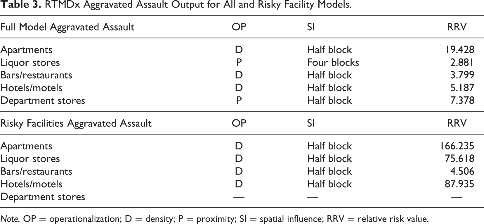
The following findings will be discussed in relation to the RTM findings and then the PAI findings for aggravated assault and theft from motor vehicles. When all facilities were input into the aggravated assault RTM, each facility type (CGA) came back as significantly (see analytical framework for RTMDx steps) related to aggravated assault (see Table 3). For example, the area within a half block of an apartment complex is about 19 times riskier for an aggravated assault than places not within a half block of apartment complexes. Similarly, being within a half block of a major chain department store is about 7 times riskier than being in places beyond a half block. The results also indicate that department stores are about twice as risky for aggravated assaults than bars/restaurants. Moreover, the influence that liquor stores have on aggravated assault risk radiates out four blocks from the establishment. The maps for the full model RTMs for aggravated assault and theft from motor vehicles are illustrated in Figures 2 and 3.
RTMDx Aggravated Assault Output for All and Risky Facility Models.
Note. OP = operationalization; D = density; P = proximity; SI = spatial influence; RRV = relative risk value.
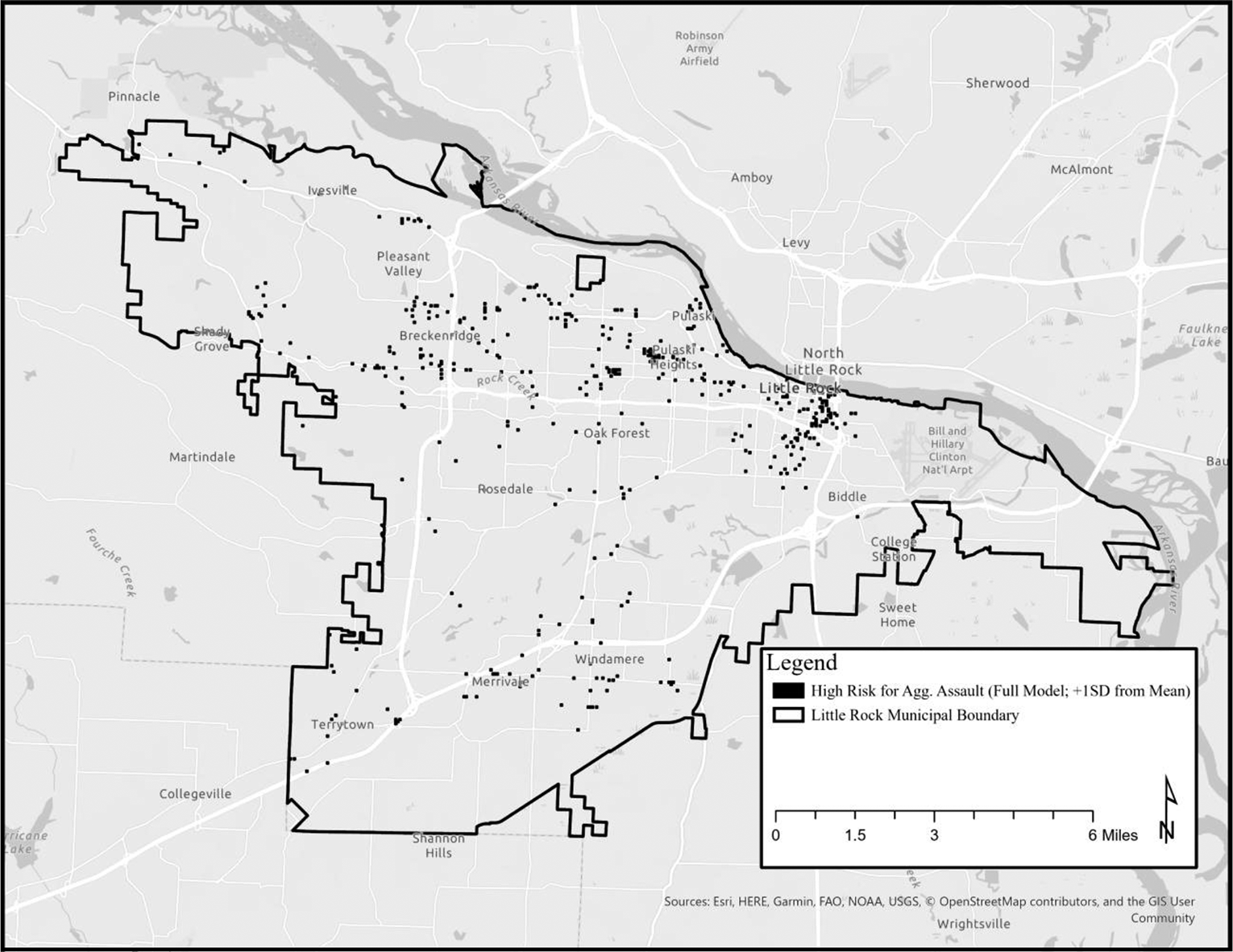
High-risk places for aggravated assault full crime generator and attractor model.
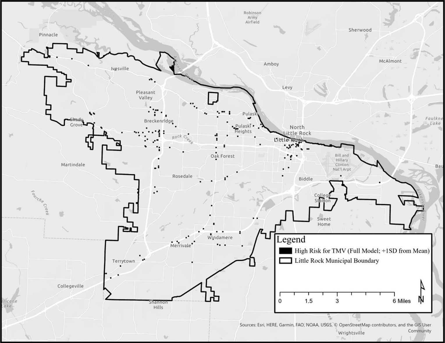
High-risk places for theft from motor vehicle full crime generator and attractor model.
Not surprisingly, once limiting the input to only risky facilities, the relative risk value for the significant risk factors increases as shown by the bottom panel of Table 3. The half block spatial influence with density operationalization results in the immediate area surrounding each facility having the greatest risk. Since the risky facility RTM used the same 2018 crime data to identify risky facilities, this should be expected since risky facilities were determined by address comparison between crime and facility addresses. See Figures 4 and 5 for the risky model RTM maps for aggravated assault and theft from motor vehicles. The exclusion of department stores illustrates the two-step process of RTMDx: Department stores are not included in the “best” model even when we restricted the CGAs to only risky facilities. The risk terrain maps for both—the full model and risky facilities model—are subsequently used to select out high-risk places (+2 SD from the mean) and compare the predictive accuracy in forecasting January through September 2019 aggravated assaults.

High-risk places for aggravated assault risky facility model.

High-risk places for theft from a motor vehicle risky facility model.
When examining Table 4 for theft from motor vehicles, similar patterns emerge. In the full CGA model, all facility types are significant and comprise the “best” model. Interestingly, department stores are the riskiest facility type. For example, the top panel of Table 4 shows that while both are risky for theft from motor vehicles, department stores are about 15 times riskier than liquor stores. Moving to the risky facility RTMDx findings in the bottom of Table 4, similar to the findings for aggravated assault, the relative risk values increase for apartment complexes, bars/restaurants, and hotels/motels, decrease slightly for department stores, and liquor stores are no longer in the “best” fitting model. The risk terrain maps for theft from a motor vehicle are also used to select places with relative risk scores greater than two standard deviations from the mean for forecasting comparison.
RTMDx Theft From Motor Vehicles Output for All and Risky Facility Models
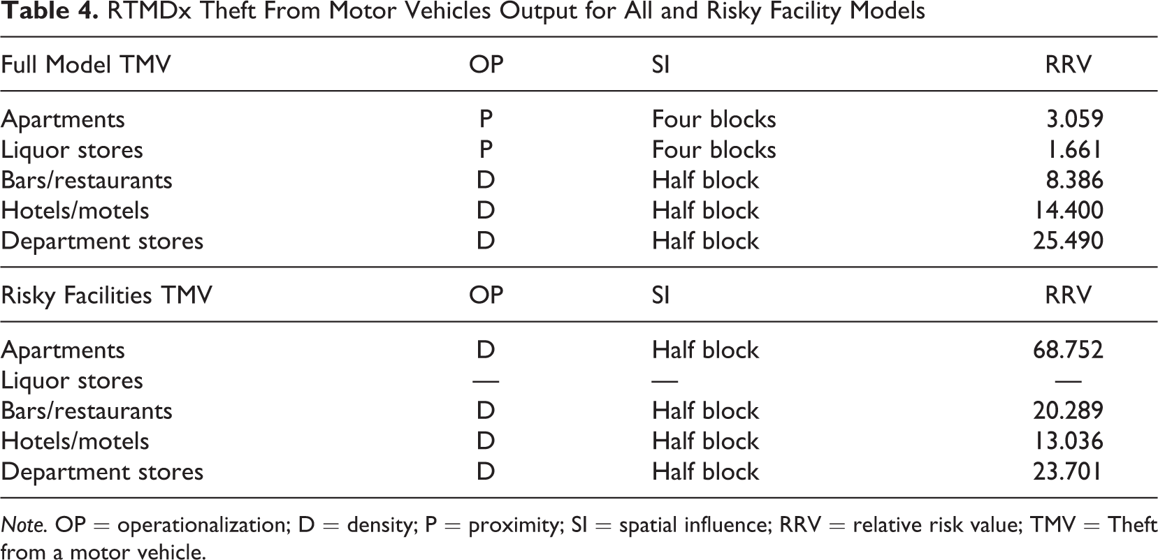
Note. OP = operationalization; D = density; P = proximity; SI = spatial influence; RRV = relative risk value; TMV = Theft from a motor vehicle.
PAI
The primary focus of the current study is on identifying whether restricting the RTM process to only risky facilities results in more accurate predictions of crime. Table 5 provides a summary of the PAI values across models and crime types. Common to both aggravated assault and theft from motor vehicles, the models limited to only risky facilities are far more accurate than the full facility models. In fact, the risky model for aggravated assault is more than 3 times more accurate than the full facility model. Moreover, the risky model for theft from motor vehicles is more than twice as accurate as the full model. It is important to note that since the input for each RTM differs based on the extent of facilities, the relationship to crime will differ. This will result in different places being identified as high-risk, greater, or lesser areas, leading to differing street lengths where crime would be expected to occur in the future. Similar results emerge when changing the denominator to cells rather than street length as seen in Table 6.
Predictive Accuracy Index (PAI) Values for Full and Risky RTMDx Models for Both Crime Types.
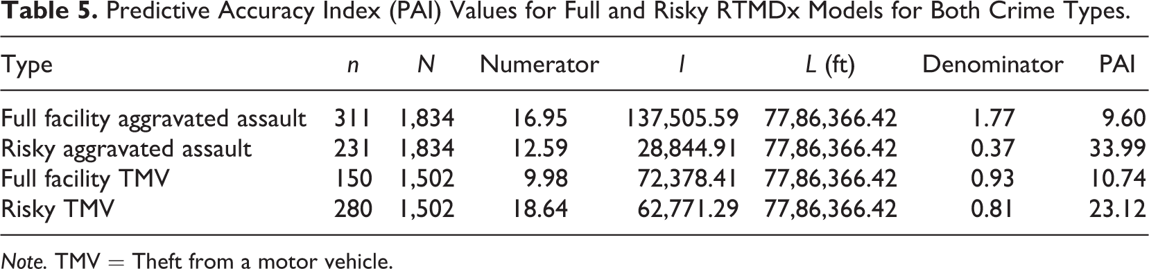
Note. TMV = Theft from a motor vehicle.
Predictive Accuracy Index (PAI) Values for Full and Risky RTMDx Models for Both Crime Types With Cells.
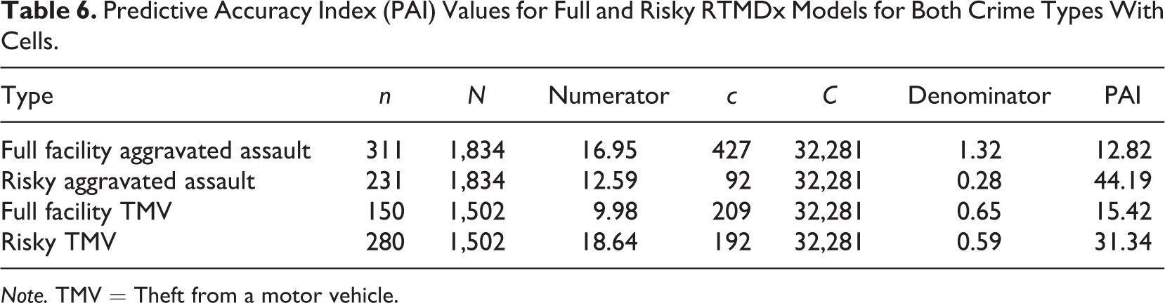
Note. TMV = Theft from a motor vehicle.
When examining the different parts of the PAI calculation, it becomes clear why the models limited to risky facilities outperform the full facility models. For aggravated assault, the full facility model captures more predicted crime, leading to a larger numerator (hit rate), but the length of streets is about 5 times more for the full facility model than the risky model. Since the full model has all facilities and differing spatial operationalizations, there is more opportunity to forecast crime but at a cost increasing the coverage area. Interestingly, when examining theft from a motor vehicle, the risky model was able to accurately predict more crime while having a smaller street length, yielding a comparatively smaller gain in predictive accuracy for the risky model.
Supplemental Analyses
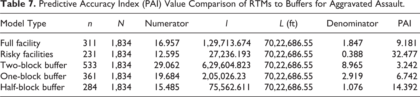
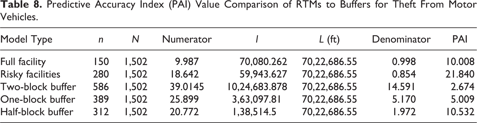
In conducting the above analyses, we considered whether the complexity of making crime predictions is necessary, given the identification of risky facilities. To that end, we took the descriptive process of identifying risky facilities for each crime type and placed multiple buffers around the risky facilities in order to compare predictive accuracy. All risky facilities for each crime type were merged before creating buffers at half-block, one-block, and two-block increments. Similar PAI calculations were completed for comparisons across models. Additionally, the total length of street segments in Little Rock was reduced based on streets having a name where unnamed streets were removed but no to/from attributes for the geocoding process to identify whether this altered findings. The crime data for the current study were geocoded within ArcGIS rather than using the longitude and latitude provided from the LRPD crime data. The geocoding process used within LRPD could return different offsets or centerline points based on their automated process.
Tables 7 and 8 provide the results of the PAI comparisons for aggravated assault and theft from a motor vehicle, respectively. Based on the change to the total streets (L), the general results remain the same: Risky facility models outperform full facility models for both crime types. Moving to the buffer comparisons, we find that when comparing the full facility RTM models to the buffers around risky facilities, the half block risky facility buffers were more accurate than a full facility RTM. As the buffer distance increases, the PAI decreases, indicating a diminishing return for both aggravated assault and motor vehicle theft. This would indicate that simply using a proximal buffer capturing crime in the nearest vicinity of risky facilities is more accurate than using a more traditional RTM approach. Importantly though, the risky facility RTM process still far outperformed the full facility RTM and the half-block buffer around risky facilities.
Predictive Accuracy Index (PAI) Value Comparison of RTMs to Buffers for Aggravated Assault.
Predictive Accuracy Index (PAI) Value Comparison of RTMs to Buffers for Theft From Motor Vehicles.
Discussion
Practitioners and researchers continue to be interested in the ability to forecast where crime occurs in order to efficiently and effectively allocate resources for the prevention and reduction of crime. The current study focused on one tool (analytical approach) to understand where crime occurs and to use that information to forecast future incidents of crime. Specifically, we utilized a fairly common concept of risky facilities to explore the predictive accuracy of different models using both the traditional RTM approach and RTM models focusing exclusively on only the riskier CGAs. Where traditional RTM approaches rely on the usage of all facilities of different types such as apartment complexes, hotels, and restaurants, long-standing observations from environmental criminology, including the 80-20 rule, suggest that only a small proportion of those places accounts for the vast majority of all crime.
The issue that arises is that, in traditional RTM approaches, all facilities of one type are treated as equal rather than acknowledging substantial variability within any facility type. The current study found, first, that identifying risky facilities paralleling the work of Eck et al. (2007) greatly increased the predictive accuracy of RTM. Results held across two substantively different crime types, aggravated assaults, and theft from a motor vehicle. When all facilities were included within RTM, a large percentage of false positives identified places as high risk when risk was in fact not high. By taking an additional analytical step to first identify truly risky facilities before utilizing the automating RTM process, the predictive accuracy doubled or even tripled depending on the crime type as seen in Table 5.
The approach used in the current study also provides a different approach to the vulnerability-exposure framework (see Kennedy et al., 2016) often associated with RTM. That is, exposure is typically the secondary thought after identifying vulnerable places at risk of future crime occurrences. This borrows from the well-established hotspot literature on identifying places where vulnerability is high and past exposure, measured through the formation of crime hotspots, overlap, identifying places at the greatest risk. The current study shifted exposure to the primary concept of interest in identifying risky facilities within each CGA type. This allowed for the RTM process to generate risk assessments based on facility subsets that are known to have crime at their specific locations. By doing so, the current study stands separately from prior approaches to assessing risk through RTM.
In addition, findings from our supplemental analysis were instructive. Given that risky facilities were already identified, the author(s) explored whether RTM was necessary or whether the risky facilities could be used with spatial buffers. Although there were diminishing returns in predictive accuracy when increasing the buffer distance around the risky facilities, the immediate area surrounding the risky facilities (half-block buffer) had a greater PAI value than the traditional RTM approach. If the focus was on predictive accuracy alone, this would indicate risky facility buffers would be a better analytical approach than standard RTM. However, using only risky facilities within an RTM process was still at least twice as accurate as all other approaches.
The outlined analytical approach in the current study still fits within the larger risk narrative discussed by Kennedy et al. (2018) in developing risk mitigation and crime reduction strategies. The risky facility step of the current study refines the discussion to a subset of facilities rather than the broader landscape of all facilities of any type. For instance, the current study examined five different facility types (CGAs) with which place management around the identified risky facilities could be enhanced to reduce or prevent crime. Indeed, the extant literature on risky facilities often includes a discussion on the role place managers have in shaping social outcomes, as well as police, on altering the attractiveness of facilities and reducing crime at those facilities (Bichler et al., 2012; Eck, 2015; Eck & Wartell, 1998; Franquez et al., 2013; Madensen & Eck, 2008). If RTM is going to be used as an analytical technique to identify places at greater risk of crime, then attention needs to be drawn to those risky facilities where most crime occurs in order to better allocate resources and/or identify stakeholders that need to be held accountable.
The current study is not without limitations. First, the analysis only examined five different types of CGAs. The process used to identify risky facilities per facility type and crime type is not an automated process (at this point). Given the findings of the current study, the author(s) believe a risky facility base for RTM would produce more accurate forecasts and future research should expand on the current study to include more CGAs. This would also allow for a comparison to recent work by Wheeler and Steenbeek (2020) finding a random forests approach outperforms RTM based upon the PAI (as done within the current study). Along the same lines, we only examined two crime types. The generalizability of the findings should further be tested to varying crime types and expanded to include calls for service to test the application beyond specifically crime-based outcomes.
Along similar lines, the current study only focused on the built or physical environment and primarily businesses in Little Rock. In turn, we exclude social factors and the influence they have on crime occurrence, even at the place level (see place in neighborhood; Wilcox & Tillyer, 2017). RTM has been used with social factors in prior research but typically at a neighborhood level (e.g., Thomas & Drawve, 2018). Thus, one limitation consistent with Weisburd et al.’s (2012) discussion on the importance of both fields of research, more consideration could be given to opportunity (e.g., routine activities theory and crime pattern theory) and social disorganization alongside built environment factors.
Based on the current study, and growing emphasis within environmental criminology more broadly, the role of risky facilities warrants greater attention in community and place, crime forecasting, and CGA research. With the advancements made within the law of crime concentration literature, including robustness and the quantification of concentration (e.g., Bernasco & Steenbeek, 2017; Favarin, 2018; Gill et al., 2017; Haberman et al., 2017; Levin et al., 2017; Mohler et al., 2019), this line of research could jointly examine the role that facilities play in the spatial patterning of crime. That is, while the law of crime concentration indicates that crime is concentrated, it fails to speak to why it occurs at certain places. Jointly examining the concentration of crime and the influence (independently or together) of risky facilities have on the concentration of crime would better equip practitioners to develop prevention strategies and more efficiently allocate scarce resources for combatting local crime problems. In going back to the roots of environmental criminology assessing CGA’s role in crime and risk of crime, this study opens the door to future research in environmental criminology concerning risk and crime in place.
Footnotes
Acknowledgments
The authors would like to thank Rutgers Center on Public Security and those at the American Society of Criminology (2019) panel for feedback and commentary. An earlier version of this study was submitted for RTM certification by H. Steinman.
Declaration of Conflicting Interests
The authors declared no potential conflicts of interest with respect to the research, authorship, and/or publication of this article.
Funding
The authors received no financial support for the research, authorship, and/or publication of this article.
