
Abstract
Simulation studies use computer-generated data to examine questions of interest that have traditionally been used to study properties of statistics and estimating algorithms. With the recent advent of powerful processing capabilities in affordable computers along with readily usable software, it is now feasible to use a simulation study to aid in clinical decision making. By simulating large quantities of data that mimic clinical situations, it is possible to understand the ramifications of different decisions better than using tangentially relevant data or intuition. In this tutorial article, I describe the general steps in conducting a simulation study with particular emphasis on clinical decision making. I conclude with a didactic example taken from clinical literature on identifying a specific learning disability.
Simulation studies use computer-generated data to examine questions of interest. Originally, the most common purposes for conducting a simulation study in education or psychology were to determine the sampling distributions of test statistics, compare parameter estimators, evaluate an algorithm, or compare multiple algorithms that perform the same function (Psychometric Society, 1979). Later, researchers found that simulation studies could also be useful in planning the sample size required for a study (e.g., Beaujean, 2014; Muthén & Muthén, 2002).
With the advent of affordable computers that have powerful processing capabilities and readily usable software, it is now feasible to use a simulation study to help with clinical decision making. In clinical practice, it is not unusual to make decisions about individuals who are normatively rare (e.g., psychiatric/education diagnosis, atypical symptoms). In these populations, often there is very limited data available to test clinical hypotheses that are generalizable beyond a single case. Consequently, by simulating large quantities of data that mimic clinical situations, it is possible to understand the ramifications of different decisions better than using tangentially relevant data or intuition. In this tutorial article, I describe the general steps in conducting a simulation study with particular emphasis on the clinical context. I conclude the article with a didactic example.
Steps in Conducting a Simulation Study
There are six basic steps required for all simulation studies (Burton, Altman, Royston, & Holder, 2006; Fan, 2012; Feinberg & Rubright, 2016; Harwell, Stone, Hsu, & Kirisci, 1996; Law, 2006; Paxton, Curran, Bollen, Kirby, & Chen, 2001).
Simulation studies can be conducted to investigate almost any type of scientific problem, but they are best used when the needed data cannot be reasonably obtained in another way. All simulation studies are based on simplified versions of reality, so they will never be able to fully replicate all the complexities involved in the problems of interest. Thus, if actual data are available—or it is feasible to collect them—then they should be analyzed instead of, or in conjunction with, simulated data.
To build a worthwhile conceptual model, gather information about the essential variables, including how the variables are related to each other and what distributions data from the variables follow. While the normal distribution is the “go to” distribution in educational and psychological research, it is not always the most appropriate. For example, Shadish and Sullivan (2011) noted that the majority of data collected in single-case research were counts (e.g., number of behaviors observed in a time period) or proportions (e.g., proportion of time intervals a behavior was observed). Thus, simulating data for these types of variables would require using alternative distributions, such as Poisson, binomial, or even a mixture of distributions.
In addition to determining information about the essential variables, creating a conceptual model also requires making simplifying assumptions about the system. This is necessary to make the conceptual model tractable for a simulation study. Unnecessary details can result in excessive execution time for the simulations or obscure aspects of the system that are really important. Typically, it is better to start with a simple model and add more complexity as needed.
In clinical situations, the model assumptions will typically be that certain variables can be excluded without substantially influencing the results, the relations among the variables are of a certain magnitude and direction, and the model residuals/errors have a certain structure. For example, if simulating longitudinal data, some typical assumptions would be that variables collected at Wave 1 are related to the same variables collected at Wave 2, and that the Wave 2 variables are not causing the Wave 1 variables. As another example, if simulating classroom behavior data, it might be a tenable assumption that the principal’s education level can be excluded from the conceptual model without substantially influencing the results.
While not required, it may be helpful to create a path diagram of the conceptual model. Not only can many clinical problems be conceptualized in terms of a path diagram (Hoyle & Smith, 1994), but creating such a diagram also requires the user to be explicit about the model’s assumptions and can also aid in the analysis of the data. Loehlin and Beaujean (2017) provide details for creating and analyzing path diagrams for a variety of common models in psychology and related disciplines.
While a bit of an oversimplification, simulation studies can be classified as either unreplicated or replicated. Unreplicated studies simulate m = 1 data set for a given set of conceptual model conditions (e.g., data distributions, parameter values, n). As only one data set is being simulated, typically, the n used for this type of design is large.
One example of an unreplicated study is Stuebing, Fletcher, Branum-Martin, and Francis (2012). They were interested in the accuracy of three different methods for identifying a specific learning disability (SLD). To do so, they simulated n = 1,000,000 observations using a single set of published correlations between scores on norm-referenced cognitive ability and academic achievement tests. As another example, Crawford, Garthwaite, and Gault (2007) showed how using unreplicated simulations with a large value of n can aid in determining base rates for score differences.
A replicated study (also called a Monte Carlo [MC] study) simulates m > 1 data sets for each set of model conditions. As multiple data sets are simulated, the n is selected to reflect either what is typically found in the system or what previous studies of system have used. Usually, multiple values for some of the conceptual model conditions are used to generate the data and then the results from the different conditions are compared.
MC studies are common in statistical research, but they are relatively uncommon in clinical studies. One example of such a study is Moreau (2014). He was interested in the influence of individual differences on working memory training interventions. To investigate this, he simulated data under a variety of conditions of how the treatment and control groups could be formed. For each set of conditions, he simulated n = 20 observations in each group, calculated the between-group differences, and then repeated the process m = 10,000 times.
If conducting an MC study, selecting the model conditions and values for m is important—and there are not absolute best values for either. On one hand, large values of m provide precise results. On the other hand—assuming a fixed amount of resources—larger values of m reduce the number of conceptual model conditions that can be investigated, which can reduce the external validity (i.e., generalizability) of the study. Skrondal (2000) advocated for choosing these values based on the individual simulation study instead of just relying on “conventional wisdom.”
The last part involved in designing a simulation study is determining how to analyze the generated data. Planning this out before starting the simulation process can not only increase the efficiency of the data analysis but will also aid in making sure the simulated data will be able to answer the questions of interest. The data analysis should include descriptive statistics, such as the mean and standard deviation (SD) of the statistics of interest across the m replications (see Table 1). In MC studies, the SD of a statistic across replications is an approximation of the statistic’s standard error; thus, it is sometimes called the empirical standard error (ESE). The ESE can be used the same way as analytic standard errors, such as examining the precision of the statistic. The ESE could be used to create an empirical confidence interval (CI) as well, but more typically CIs are created in MC studies by rank ordering the m statistics and finding values at the desired percentiles (Buckland, 1984).
Summary Statistics and Performance Measures for Simulation Studies.
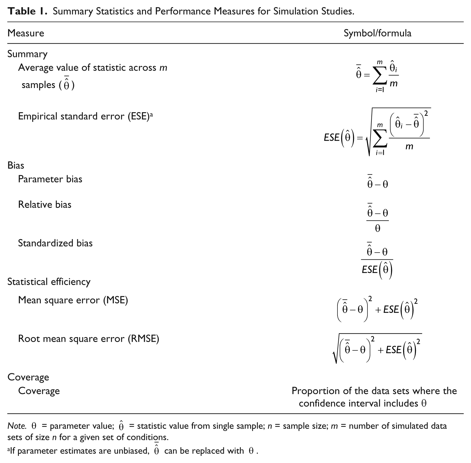
Note.
If parameter estimates are unbiased,
The data analysis for most simulation studies should go beyond descriptive statistics. Because researchers have full control over the parameter values examined in a simulation study, many have advocated for treating simulation studies—especially MC studies—as experiments. Thus, they argue that simulation studies should use appropriate experimental designs, validity checks, and data analyses techniques (e.g., Harwell, 1997; Skrondal, 2000).
Simulating data can be done in a general-purpose programming language (e.g., Python, C++), many statistical programs (Lee, 2015), as well as some specialized simulation programs. For example, in the next section, I used the R program (R Development Core Team, 2016). I did so because it is free, and there are many packages available to conduct most analyses that are of interest for examining clinical data.
When simulating the data, start by creating some pilot data using small values for n and m (if conducting a MC study) along with one or two sets of parameter values. Use these data to check for adequacy of data, such as the absence of impossible values, reasonable values for the sample statistics, and the performance measures discussed in Step 5. If the data are not being simulated as expected, this may indicate that the program needs to be debugged.
Once you are sure the data are being simulated correctly, simulate the m desired data sets of size n. Be sure to store the necessary information from each of the m data sets so that you do not have to repeat the simulation process at a later date. For unreplicated studies, it will usually be possible to save each of the simulated data sets. For MC studies, it may not be feasible to save each data set—it depends on size of m, n, and the number of conceptual model conditions. If saving all the data sets is not feasible, then save the necessary information from each of the m iterations before the simulation procedure discards them. The necessary information will be values required for the desired data analysis as well as that needed to check the validity of the results (see Step 5).
Validating the simulation process is similar to validating the use of test scores in that there is not a single statistic that will give you this information; instead, you need to gather multiple pieces of information and make decisions based on all the evidence available. One source of evidence (results validly) comes from comparing results from the simulated data with results from data generated from the actual existing system. Of course, this assumes that data are available from the existing system, which may not be the case. Another source of evidence (face validity) comes from determining whether the simulation results are consistent with how you perceive the system should operate based on what you learned in Step 2.
A third type of validity evidence comes from gathering data from performance measures, which compare the simulated results with the parameter values used to simulate the data. The three most common performance measures examine bias, efficiency, and coverage—although there are many others available (see Bandalos & Leite, 2013; Burton et al., 2006; Muthén & Muthén, 2002). I discuss each of the performance measures conceptually and provide the formulae in Table 1. Except for bias, they all require m > 1, so it can only be estimated for MC studies.
In statistics, bias is the difference between a statistic’s value (estimated from sample data) and the value of the population parameter. Thus, calculating parameter bias requires subtracting the value of the parameter from the mean value of the statistic used to estimate the parameter across the m data sets. In an unreplicated study, m = 1; therefore, parameter bias is estimated from a single data set.
The problem with calculating parameter bias is that the scale depends on the metric of the parameter, so determining severity is difficult. Thus, it is common in simulation studies to transform the scale of the bias measure to a proportion. One method (relative bias) requires dividing the bias value by the value of the parameter, which works as long as the parameter value is not zero. An alternative for MC studies (standardized bias) requires dividing bias by the ESE. No matter what bias measure is used, smaller values indicate less bias.
Statistical efficiency is related to the statistic’s sampling variance, with less variability being more preferred. One measure of efficiency is the mean square error (MSE), which is the sum of the squared parameter bias and squared ESE (i.e., empirical sampling variance). If there is bias, then MSE represents the overall accuracy of the parameter estimation. If there is no bias, then MSE is a measure of the sampling variance of the statistic. The square root of the MSE (RMSE) transforms the MSE back onto the same scale as the parameter, which makes interpretation somewhat easier. If there is no bias, MSE ≈ ESE.
Confidence interval coverage is the proportion of samples in which the parameter value is contained in the statistic’s CI. The coverage should be approximately equal to the nominal coverage rate (e.g., 95% of the m samples for a 95% CI). Under-coverage (i.e., coverage << .95 for a 95% CI) indicates that the CI is too narrow, which results an increase in finding effects when they are not there (i.e., type I errors). Over-coverage (e.g., coverage >> .95 for a 95% CI) indicates the CI is too wide, which results in an increase of not finding effects when they are there (i.e., type II errors).
In addition to performance measures, it may be useful to conduct a sensitivity analyses, especially for unreplicated studies. A sensitivity analyses involves slightly changing the values of parameters of interest to see how the outcomes (or performance measures) change. If there is a substantial change, this would indicate that those aspects of the model have a large influence on the results so their values should be selected very carefully.
Example
Macmann, Barnett, Lombard, Belton-Kocher, and Sharpe (1989) were interested in studying the dependability of actuarial methods to identify an SLD using the discrepancy model. While this question is now somewhat outdated, they simulated data for part of their study and provided enough details so that it can be replicated.
This problem is well suited for a simulation study. First, there is currently no “gold standard” criterion for SLD, so it is impossible to determine any given method’s true accuracy. Second, although Macmann et al. (1989) were able to collect “real” data, the sample sizes were small (ns ranging from 106 to 298) and consisted only of students referred for evaluation of a suspected SLD. Thus, these results have questionable generalizability.
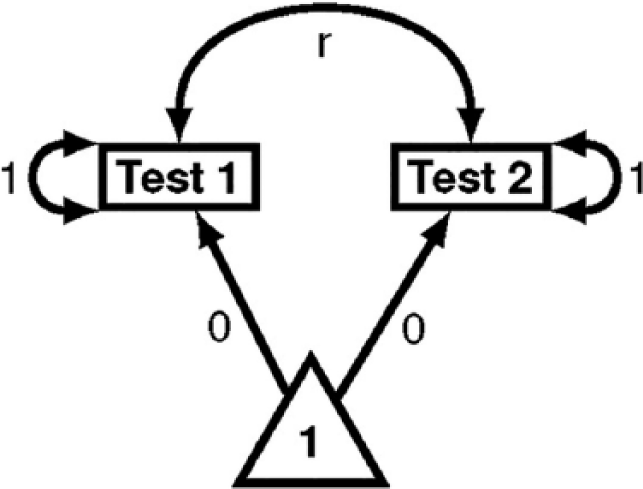
Path diagram of Macmann, Barnett, Lombard, Belton-Kocher, and Sharpe’s (1989) conceptual model.
Macmann et al. (1989) conducted an unreplicated study, simulating m = 1 sample of n = 5,000 individuals for each set of model conditions (see Table 2). While I replicate this scenario, I also extend the design to an MC study. I do this by simulating m = 5,000 samples of n = 200 for each set of model conditions. The value of n was taken to represent the sample sizes Macmann et al. reported for their student data.
Model Condition Values for Macmann, Barnett, Lombard, Belton-Kocher, and Sharpe (1989) Study.
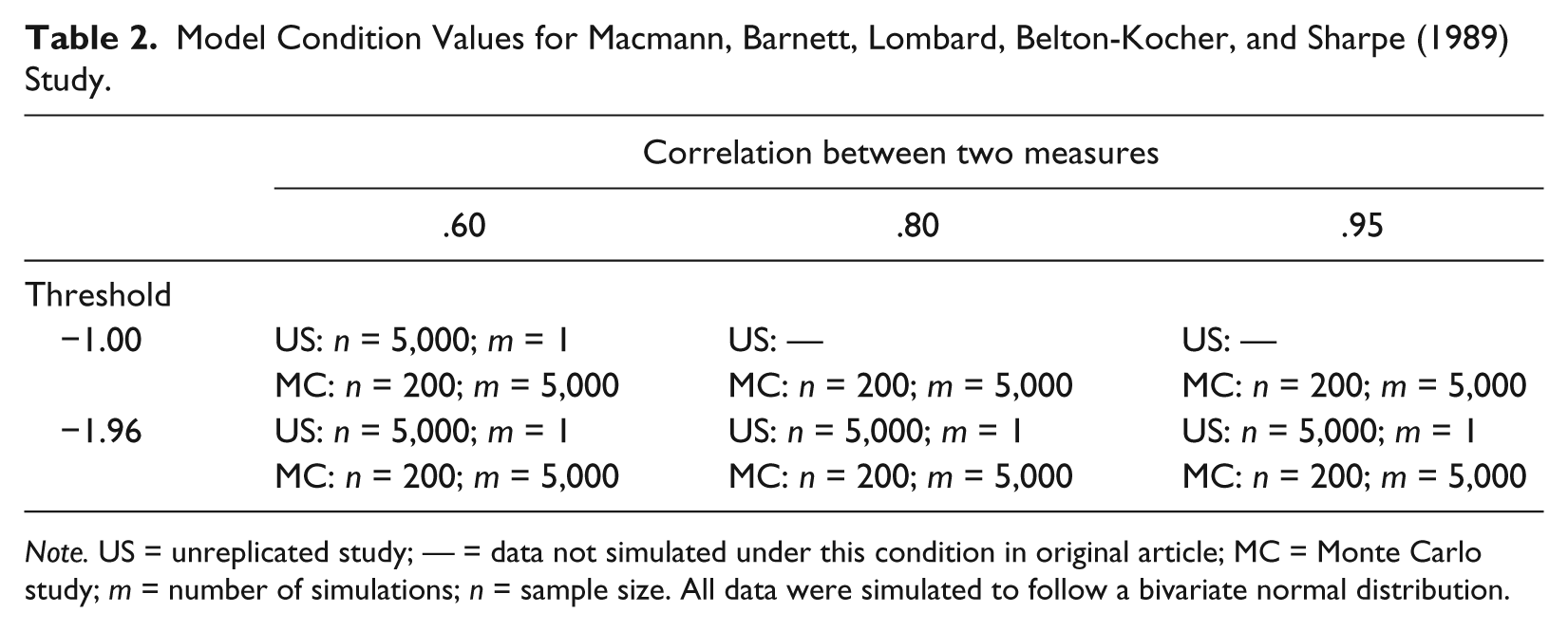
Note. US = unreplicated study; — = data not simulated under this condition in original article; MC = Monte Carlo study; m = number of simulations; n = sample size. All data were simulated to follow a bivariate normal distribution.
Agreement Data From Macmann, Barnett, Lombard, Belton-Kocher, and Sharpe (1989) and Current Study.
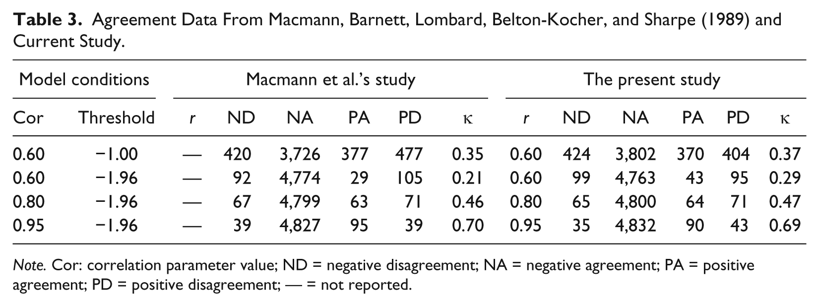
Note. Cor: correlation parameter value; ND = negative disagreement; NA = negative agreement; PA = positive agreement; PD = positive disagreement; — = not reported.
For the MC study, some of the simulated data sets did not have values for each cell of the agreement matrix, which produced a missing value for κ. For those data sets, I removed all the observations and resimulated a new data set so that each condition had m = 5,000 data sets. The results from the MC study are in Table 4. The left part of the table gives the values from the performance measures; the right part gives summary statistics for the m = 5,000 κ values simulated for each model condition.
Results From Monte Carlo Study With n = 200 for Each Condition.

Note. See Table 1 for description of performance measures and summary statistics. Cor = correlation parameter value;
The performance measures indicate that the MC simulations created good sample data: The bias is minimal (<.00 for each condition), the MSE is low, and coverage is between .94 and .95 for the 95% CI. The average of the kappa values from the MC study are similar to the values from the unreplicated study, with any differences likely due to sampling because the MC study used a much smaller n than the unreplicated study. In addition to the average value of κ, the MC study provides an indication of κ’s sampling variability. For example, for the model conditions of r = .60 and a −1.00 threshold, the average value of κ is .35 and ESE is .09. Although not shown in the table, the values for κ at the 2.5 and 97.5 percentiles are .18 and .53. These are the values for the lower and upper bound of the empirical 95% CI. Thus, if the true correlation between tests used for SLD identification was .60 and was evaluated across 200 students using a threshold of −1.00 for diagnosis, it would not be uncommon to find a κ value ranging anywhere from .18 and .53.
This MC analysis can extend beyond descriptive statistics to compare the values of κ across the conditions. For example, a two-way ANOVA (correlation by threshold) shows that there are differences between κ values across the model conditions. The most prominent factor in these differences is the correlation between the measures (i.e., higher correlations produce higher κ values), although the threshold used also contributes to agreement differences (i.e., lower thresholds produce higher κ values). The generalized eta-squared (
The results from both the unreplicated and MC studies show that SLD classification reliability using the discrepancy model is generally low for the conditions used in Macmann et al.’s (1989) study. Kappa levels can be made more acceptable by using measures that are strongly correlated (i.e., r = .95) or using lower diagnostic thresholds, but these conditions are typically uncommon in clinical practice. Thus, Macmann et al.’s main conclusion—the problems with using score discrepancies for SLD classification cannot be resolved through using “better” measures or statistical formulae—applies here as well. Moreover, their suggestion of creating expectancy tables to describe the effects of score correlation and cutoff values on classification agreement—for situations were using aptitude-achievement discrepancies is required by administrative policy—is essentially produced in the right part of Table 4. In the absence of “real” agreement data for a given set of tests scores, such a table could easily be extended to include other model conditions as well as other measures of classification agreement.
Summary
Simulation studies can be powerful tool for understanding the essential aspects of psychological and educational systems. While historically these methods were not accessible to clinicians or clinically oriented researchers, this is no longer the case. The availability of computers with powerful processing capabilities along with readily usable software have allowed simulation studies to be part of studying clinical decision making. While simulated data will never be able to replace data actually collected from the variables of interest, they are well suited for situations where it is not feasible to collect the necessary data. Hopefully, this tutorial article can aid individuals in using simulation studies to aid in understanding such problems.
Footnotes
Appendix
This appendix provides R syntax to conduct the simulation studies described in this article. The syntax uses loops and is designed for didactic purposes, making it functional but not computationally efficient. For information on writing more efficient R syntax to simulate data, see Hallgren (2013) or Robert and Casella (2009).
For both the unreplicated and MC studies, I only analyze data from one of the model conditions. Analyzing the other data sets requires straightforward modifications of the syntax. In R, NA is used to indicate missing values, so I abbreviate negative agreement using NegA. Any line starting with a pound symbol (#) is a comment.
Declaration of Conflicting Interests
The author(s) declared no potential conflicts of interest with respect to the research, authorship, and/or publication of this article.
Funding
The author(s) received no financial support for the research, authorship, and/or publication of this article.