Precision of Single-Skill Math CBM Time-Series Data: The Effect of Probe Stratification and Set Size

Abstract

Comparatively little research exists on single-skill math (SSM) curriculum-based measurements (CBMs) for the purpose of monitoring growth, as may be done in practice or when monitoring intervention effectiveness within group or single-case research. Therefore, we examined a common variant of SSM-CBM: 1 digit × 1 digit multiplication. Reflecting how such measures are often used in contemporary research and practice, we examined the comparative reliability of three representative SSM-CBM set sizes of 8, 16, and 32 unique problems. In a separate study, we investigated the possible benefit of stratifying problems within operation and probe relative to random assignment. Findings suggest that SSM-CBM slope reliability benefits from explicit stratification and that set size is a relevant consideration. Implications for the selection and interpretation of SSM-CBMs when engaging in practice and research are discussed.

Keywords

reliability measurement curriculum-based assessment education assessment elementary education/childhood mathematics longitudinal response to intervention (RTI)/multi-tiered system of supports (MTSS)

Curriculum-based measurement (CBM) materials include brief measures that are used by teachers, school staff, and researchers to assess students’ mastery of curriculum goals for the purposes of screening, progress monitoring, and decision making (Deno, 1985, 1986). Research has examined CBM in the areas of reading and math; however, the overwhelming emphasis has been on the former, despite enduring and severe math skill deficits of students in U.S. schools (National Center for Educational Statistics, 2018). The objective of the current study is to advance understanding of math CBM (M-CBM), both for research and practice. Specifically, our primary objective was to examine measurement error as it relates to the calculation of slope for single-skill math CBM (SSM-CBM) probes. We further examined how such estimates are moderated by common features of probe construction, including instructional set size, which can be defined as the number of unique math problems tested on a given probe, and stratification of items within probe.

Defining Measurement of Basic Math Skills

SSM-CBMs include problems of a narrowly conceptualized behavior (e.g., 1 digit × 1 digit multiplication). Such measures are typically used when progress monitoring individual whole-number math skills. In contrast, multiple-skill math probes consist of problems that vary in operation and difficulty and reflect overarching grade-level objectives (Christ & Vining, 2006; Hintze et al., 2002). The scoring of multiple-skill probes typically entails weighting the score value of problems by difficulty and individual problems are scored correct or incorrect (e.g., aimsweb, 2012). In contrast, for SSM-CBMs, each problem is hypothesized to be of equivalent difficulty and typically each numeral calculated correctly in the answer space is considered an instance of the target behavior, the most common index of this being digits correct per minute (DCPM; Deno & Mirkin, 1977; Shapiro, 2011). Both types of M-CBMs are offered by major vendors of CBM materials, and several free probe constructors for SSM-CBMs exist (e.g., Intervention Central, Math Facts Café).

Precision of Slope for SSM-CBMs

Christ and Vining (2006) and Hintze et al. (2002) examined the precision of SSM-CBMs, where the intended use of such measures was for screening using either normative (i.e., as compared with peers) or criterion-referenced (i.e., as compared with a benchmark) heuristics. However, the issue of measurement precision extends to the use of such probes within a research context and to progress monitoring as well. Numerous repeated-measures group- and single-subject design studies have evaluated remedial strategies to improve accuracy and fluency in whole-number operations and have used SSM-CBM as a primary or sole outcome measure (e.g., Codding et al., 2007; Hawkins et al., 2009; Poncy et al., 2012).

Probe construction employed in this representative research varies in approach. For example, several single-subject intervention studies reported using the previously described online probe builders to generate their SSM-CBMs (e.g., Hulac et al., 2012; Lannie & Martens, 2008; Mong & Mong, 2012). These probe builders generally allow user input on operation, set size, and possibly problem selection, and appear to construct probes using randomized assignment. Other authors reported manually assembling probes using a more methodical approach. For example, Poncy et al. (2012) described constructing subtraction probes where “double” problems (e.g., 8-4 = 4) were balanced across the probe sheet and block randomization of problems occurred across the first and second half of the page. As another example, Musti-Rao and Plati (2015) included 12 unique multiplication problems on each of their probes, and each was randomly positioned 3 times, once in each of three equally sized blocks across the page.

These varying approaches to probe construction likely lead to different levels of associated precision when estimating growth, where precision of slope can be estimated by the standard error of the estimate (SEE) and standard error of beta (SE_b; Christ, 2006; Cohen et al., 2003). The SEE is the average absolute difference between predicted and observed scores for the regression (i.e., a given progress monitoring case). The SE_b, which has the SEE in the numerator and is standardized by the SD of the progress monitoring duration (i.e., the predictor of interest) and sample size, is the sampling error about the slope weight (Christ, 2006). In both cases, smaller values are better (greater precision) and are judged against the magnitude of the coefficient. Precision has direct implications for the prevalence of decision-making errors within applied practice (i.e., Response to Intervention). Probes with lower precision will necessitate a longer duration of progress monitoring required to achieve a reliable estimate of slope (Christ, 2006). This also leads to difficulty when comparing the effectiveness of two interventions within a research context. Two similar studies may result, given comparable levels of power, in different outcomes (i.e., confirmation or non-confirmation of hypotheses) based on the levels of residual error associated with the specific variation of SSM-CBM utilized. This would affect both visual analysis (observed variability of the outcome across time) and traditional hypothesis testing. We examined two easily manipulated features of CBM-SSM probe construction that extant research suggests may influence precision: item arrangement and set size.

Item Arrangement

Christ and Vining (2006) and Methe et al. (2015) investigated the use of a stratified item arrangement relative to randomized item arrangements when using mixed skill M-CBM probes to estimate grade-level math ability. In Christ and Vining (2006), structured probes were created where each column consisted of the same type of math problem and, therefore, each row included one of each type of problem, as defined by each column. The authors then applied generalizability theory to calculate the proportion of variance explained by the students’ true performance relative to measurement error for both conditions. Methe et al. (2015) employed a similar research design. In both studies, results favored the stratified probes relative to the randomized probes. The difference between the two conditions in both studies was moderate, but nonetheless consistently favored the stratified arrangement.

Christ and Vining (2006) mentioned the possibility of using a stratified item arrangement for SSM-CBM probes but suggested that a random item arrangement is likely sufficient due to the narrower content that is represented on such probes. However, others have expressed concerns related to the precision of SSM-CBM time-series data for instructional decision making (Methe et al., 2015; Solomon et al., in press). Stratifying within SSMs could potentially be a feasible way to increase precision on these probes by increasing the consistency of difficulty across their various iterations. For example, it is possible that students acquire different multiples at different rates (e.g., ×2’s and ×5’s vs. ×6’s and ×8’s) when learning 1 digit × 1 digit multiplication facts, contributing to variability in student performance on SSM-CBM probes if one probe features more or less of a given multiplier than another probe (Burns et al., 2015). This would then contribute to lower levels of precision when progress monitoring. Although several empirical intervention studies have used some level of stratification in generating SSM probes (e.g., Musti-Rao & Plati, 2015; Poncy et al., 2012), the possible benefit of such relative to randomized item arrangements is unknown and therefore is a focus of the current study.

Influences of Set Size

Although SSM-CBMs index proficiency for an individual operation, there is no clear guidance as to how much of that operation should be sampled on a given probe when students undergo relevant instruction, and how this might affect slope precision. The number of unique problems tested and targeted for intervention, in contrast to the number of overall problems on the probe page(s), is known as the set size (Poncy et al., 2015). For example, if one wished to index mastery of all 1 digit × 1 digit multiplication problems for a given multiplier with positive solutions, the set size would be 10, but the overall number of problems on the page might be 48, where each problem is presented, on average, about 5 times across eight rows. It may be that larger set sizes are more precise when the duration of progress monitoring is held constant because they sample a broader swath of the target behavior relative to smaller set sizes. For example, Poncy et al. (2012) specified 21 or 22 subtraction problems per condition, and thus to monitor growth, whereas Musti-Rao and Plati (2015) elected for samples of 12 multiplication problems and Codding et al. (2007) sampled 49 multiplication problems.

Specified set size is typically determined by either study or intervention objectives. In other words, decisions regarding set size are tied to instructional intent or the necessity of dividing families of problems into equivalent groups to monitor different experimental conditions (i.e., adapted alternating treatment design; Sindelar et al., 1985), and construction of the specific probes follows. However, if the precision of slope associated with the data differed across probes as a function of set size, then this has implications for how empirical studies could be compared (i.e., knowing that one study used a more reliable outcome than another similar study), as well as the duration of progress monitoring required within an applied context. Therefore, we also examined the effect of differing levels of set size on the precision of slope for SSM-CBMs.

Current Study

There is little information on the precision of slopes for SSM-CBMs, and this knowledge serves an important role in determining the duration of progress monitoring for instructional decision making and for consideration of research design. The representative set sizes of SSM-CBMs, typically determined prescriptively or as a means to intensify intervention, may influence the precision. As well, whether a probe is stratified, as opposed to randomized, in its item arrangement likely affects the precision of slope, and both approaches are employed in the extant literature. The purpose of the current study was to explore the precision of slope for several variants of 1 digit × 1 digit multiplication SSM-CBMs, a common whole-number operation targeted in the empirical literature (e.g., Codding et al., 2007; Musti-Rao & Plati, 2015; Poncy et al., 2013). This inquiry was organized into two similar and separate studies: one examining the effect of probe stratification (Study I) and one examining the effect of set size (Study II). Our specific research questions were as follows:

Research Question 1: Does the specified set size affect the precision of slope of SSM-CBMs, measured as the SEE and SE_b of the linear trendline describing growth across time?

Research Question 2: Does the use of a stratified item arrangement improve the precision of slope of SSM-CBMs relative to a randomized item arrangement, indexed as the SEE and SE_b of the linear trendline?

Our hypotheses were that larger set sizes and stratified item arrangements would yield more precise slopes relative to smaller set sizes and randomized item arrangements, aligning with prior work. As forms of exploratory analysis, we also examined growth across multipliers.

Method

A within-person longitudinal design was used to evaluate our hypotheses. In Study I, the independent variable was SSM-CBM item arrangement, which had two levels: stratified or randomized item arrangement. In Study II, the independent variable was set size, which had three experimental levels: set sizes of 8 (SET8), 16 (SET16), or 32 (SET32). These set size ranges were selected as they represent plausible conditions found in the published literature (cf. Flores, 2010; Hintze et al., 2002; Windingstad et al., 2009). Furthermore, the largest set, SET32, represents a sizable portion of all available problems for the given operation and likely behaves similarly to a probe that samples randomly from the universe of all possible problems. Similar to past early trajectory CBM research, this study assessed students as they proceeded in their general education curriculum (e.g., Ardoin & Christ, 2009; Christ, Zopluoglu, Monaghen, & Van Norman, 2013).

Participants

In Study I, participants were 34 third-grade students in general education within two classrooms at an urban public elementary school in the Northeast. In Study II, participants were 54 third-grade students in three separate classrooms in the same school. These sample sizes align with previous studies on slope precision (cf. Ardoin & Christ, 2009; Thornblad & Christ, 2014). Data were collected over 10 weeks during the fall of 2018. Standardized test results from the 2017–2018 school year indicated that 34% of third graders were considered proficient in English language arts while 47% were considered proficient in mathematics. The following demographic information for all students at the school was available from the previous school year: 40% White, 15% Black, 14% Hispanic, 7% Asian, and 15% Multiracial; 49% female and 51% male; 76% of students were considered economically disadvantaged; and 4% were English Language Learners.

The math curriculum employed was Go Math! (2015). The publishers describe the curriculum as being aligned with both Common Core and the National Council of Teachers of Mathematics curriculum standards. A manual review suggested that the fall of third grade is marked by continuing instruction on multidigit addition and subtraction from second grade and introduction to 1 digit × 1 digit multiplication. Teachers reported instruction begins with initial conceptual (i.e., use of models and demonstration with manipulatives) and procedural knowledge (i.e., skip counting) with multipliers. This was followed by procedural and fluency-based exercises that focused on small groups of multipliers sequentially (×0–×2, ×3–×5, ×6–×9), all of which began during the course of the study.

Procedures

Data collection began the third week of October 2018, which was identified by the lead teacher as being the start of 1 × 1 multiplication instruction, and subsequently took place on Mondays and Thursdays for 10 weeks. Data collection ended after 10 weeks due to the occurrence of the school’s winter holiday recess and because this length (a) is similar to the duration of other progress monitoring and math intervention studies, (b) reflects a maximal length of time that teachers would likely consider modifying instruction to address student needs, and (c) covered the time in which all multipliers were introduced in the curriculum. We included multipliers from ×2 to ×9, as multipliers of ×0 and ×1 can be solved with simple procedural knowledge (Poncy et al., 2010).

Standard administration directions were read to students at the start of each session and then probes were group administered. Students were given 2 min to complete each probe (Christ & Vining, 2006; Duhon et al., 2015; Hintze et al., 2002). At the end of 2 min, students were instructed to stop and turn to the next probe. During assessment, data collectors walked around the classroom to monitor and redirect students if they were off-task or skipping problems. Assessment sessions not able to be held on Mondays or Thursdays were held on the following school day. Individual students did not make up missed sessions.

Data collectors included doctoral- and master’s-level school psychology graduate students. A 1-hr training on the administration of M-CBM was provided to all data collectors prior to commencement of the study, which included practice exercises on SSM-CBM probe scoring. Data collectors were provided explicit, scripted directions for how to introduce the task to students and how to monitor students’ on-task behavior. These directions were reviewed in the training and then provided every data collection session.

In Study I, the two SSM-CBM probes—one stratified, one randomized—were administered each assessment session in counterbalanced order. During the course of the study, two students reached the maximum score on at least one of these probe conditions. These students were given a second sheet of problems the next day after achieving the maximal score and directions were altered accordingly. For Study II, three probes were administered in counterbalanced order. Seven students reached a maximum score, the earliest in Week 6, during the course of the study, and identical adjustments were made.

Measures

Probes consisted of 1 digit × 1 digit multiplication problems with multiplicands and multipliers ranging from ×2 to ×9. Probes were developed using a random problem generator created for the purposes of this study in Microsoft Excel. Vertically aligned problems were printed in black using 16-point Arial font. Student performance was measured using DCPM. DCPM signals the number of digits written in the proper column of the answer space, summed across available problems (Burns et al., 2006; Deno & Mirkin, 1977; Shapiro, 2011).

Study I

Probes included 48 problems arranged in eight columns and six rows. The randomized probes consisted of problems with multipliers and multiplicands randomly selected between ×2 and ×9. Randomization occurred each session and across classrooms. In contrast, the stratified probes were arranged such that the multipliers were stratified in a Latin-square design using digits between 2 and 9 (i.e., first row: ×2, ×3, ×4, ×5, ×6, ×7, ×8, ×9; second row: ×3, ×4, ×5, ×6, ×7, ×8, ×9, ×2; third row: ×4, ×5, ×6, ×7, ×8, ×9, ×2, ×3, etc.), while the multiplicands were randomly selected digits between 2 and 9. This specific arrangement was chosen because, in the first row, students first got the opportunity to answer questions reflecting content first learned in their curriculum unit (i.e., multipliers of ×2, then ×3, then ×4, etc.), increasing the probability that students would be able to demonstrate mastery of content already learned and thus the sensitivity of the instrument.

Study II

The three SSM-CBMs were each comprised of a random selection of 1 × 1 multiplication problems of multipliers ×2 through ×9. Prior to the experiment, multiplication problems were resampled for each teacher without replacement and assigned to the three conditions using a random problem generator created for the study until all conditions were full (i.e., 8, 16, and 32 selected problems, respectively). The probes featured 64 problems in an 8 × 8 array on portrait-oriented 8.5 × 11 in. paper, with each problem randomly selected from the defined sets described above.

Analysis

Student-level analysis

Our primary objective focused on the precision of estimation at the individual student level. Therefore, in line with common practice, the ordinary least squares (OLS) SEE and SE_b were calculated for each student and then aggregated to evaluate the precision of progress monitoring slopes (Ardoin & Christ, 2009; Christ, 2006). The SEE signals the absolute magnitude of the residuals about a given students’ progress monitoring slope. In contrast, the SE_b signals the width of the sampling distribution for the parameter indicating slope. The SEE and SE_b were calculated for monitoring durations of 3, 6, and 10 weeks to reflect different progress monitoring durations. The time predictor was coded such that a one-unit increment corresponded to one additional week of monitoring. These values were then contrasted in a series of analyses of variance (ANOVAs) across both studies.

Group-level analysis

Time-series multilevel modeling (MLM) with restricted maximum likelihood estimation was used to estimate the group-level slope values as a form of secondary analysis. The associated random effects signal the distribution of growth rates across students and were of interest, as was the reliability of the Level 2 parameters, which speak to the ability to make norm-referenced decisions with the slope data. A two-level model was defined with individual data points nested within students, with a predictor for weekly change in scores (time) at Level 1. Prior to analysis, we examined whether a linear or quadratic trend best fit the data for each condition. This model assumes that residuals at Level 1 and Level 2 follow a normal distribution with mean of zero.

Results

Interobserver agreement was conducted for a random selection of 20% of scored probes across all conditions. Agreement was 99%. Approximately 7% of the data were missing. The median number of missing data points across students was one, with two students incurring 4 missing days and two students 6. The median number of missing data points across sessions was 3, with a maximum of 7. In other words, no specific subject or time appeared to be an outlier regarding missing data, and missing data were fairly low across subjects and time. For all analyses, missing data were handled via list wise deletion.

Study I: Influence of Stratification

Precision of slope

SEE and SE_b values across conditions and duration of progress monitoring are shown in Table 1. Overall, precision across conditions ranged, at a practical level, from moderate to high. For example, if one monitored for 3 weeks using randomized probes, the 80% margin of error would be ±1.22 DCPM/week, where the average SE_b was 0.95 relative to the estimate of slope of 4.25 DCPM/week (Table 1). In contrast, the same margin of error for stratified probes across 10 weeks of monitoring would be ±0.37 DCPM/week, where the SE_b was 0.28. Inspection of Table 1 shows a pattern of superiority across both statistics for the stratified condition, with differences of between 0.38 and 0.79 for the SEE, and 0.04 and 0.16 for the SE_b. A repeated-measures t tests confirmed these findings. Specifically, the difference between the two conditions was significant for 6 weeks, t = 4.62, p < .001, d = 0.78, and 10 weeks, t = 3.85, p ≤ .001, d = 0.65, and approached significance for 3 weeks of data, t = 2.00, p = .054.

Table 1.

SEE and SE_b for Randomization and Stratification Conditions.

	3 weeks		6 weeks		10 weeks
Parameter	Randomized	Stratified	Randomized	Stratified	Randomized	Stratified
SEE
${\bar{X}}_{S E E}$	2.33	1.95	3.63	2.85	4.07	3.58
SD_SEE	1.04	1.39	1.08	0.92	1.03	1.02
SE_b
${\bar{X}}_{S E_{b}}$	0.95	0.80	0.58	0.46	0.32	0.28
$S D_{S E_{b}}$	0.42	0.57	0.17	0.15	0.08	0.08
Skew_SEE	1.19	2.37	0.34	1.25	0.35	1.12
Kurt_SEE	1.69	7.90	−0.03	3.01	−0.43	1.20

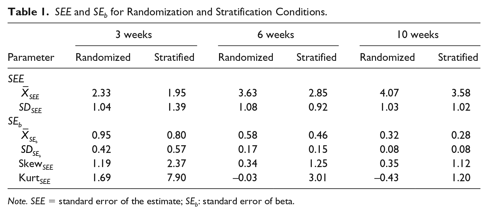
Note. SEE = standard error of the estimate; SE_b: standard error of beta.

Modeling of group tendencies

Level 1 and Level 2 residuals were inspected and found to be approximately normal, as was the distribution of the outcome variable. The average student gained about 4.00 DCPM/week collapsed across conditions (see Table 2). However, the variance components suggested this growth was highly variable. For example, for the stratified condition, a range of growth across students of −1 to 1 SD equaled 1.45 to 6.43 DCPM/week, highlighting the wide range of response to exposure to the curriculum. Both conditions yielded equal reliability of .94 for the Level 2 slope estimates, suggesting patterns of growth could be reliably attributed to individual students.

Table 2.

Results From the MLM for Randomized and Stratification Conditions.

Description	Coefficient	b	SE	t	df	p
Randomized
Intercept	β₀₀	1.94	1.19	1.63	34	.11
Time	β₁₀	4.25	0.46	9.26	34	<.001
Stratified
Intercept	β₀₀	2.83	1.01	2.81	34	.008
Time	β₁₀	3.94	0.43	9.11	34	<.001
Variance components (reported as SD)
	Intercept (reliability)	Time (reliability)	σ	Deviance
Randomized	5.52* (.61)	2.63* (.94)	8.34	4,539.79
Stratified	4.55* (.59)	2.49* (.94)	7.34	4,399.82

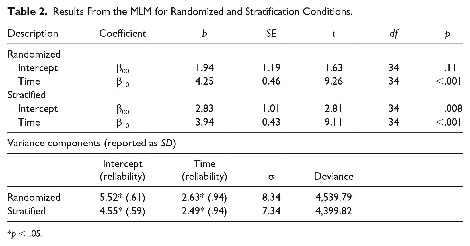
p < .05.

Exploratory analysis—Multiplier difficulty

Additional analyses were conducted to examine potential differences in students’ responding to individual multipliers. This was done because this may explain why a difference between item arrangements was found. Student responses on probes administered during the initial 2 weeks, and final 2 weeks of data collection were averaged and examined within the stratified item arrangement. The average number of problems answered correctly for each multiplier is shown in Figure 1. The figure also shows the proportion of students who correctly answered two or more problems of each multiplier. The results of this analysis revealed variation in students’ responding. Specifically, problems containing the multiplier ×5 were correctly answered at a higher rate than all other multipliers both at pre- and post-test. In contrast, multipliers of ×8 appeared to be the most difficult for students at the post-test.

Figure 1.

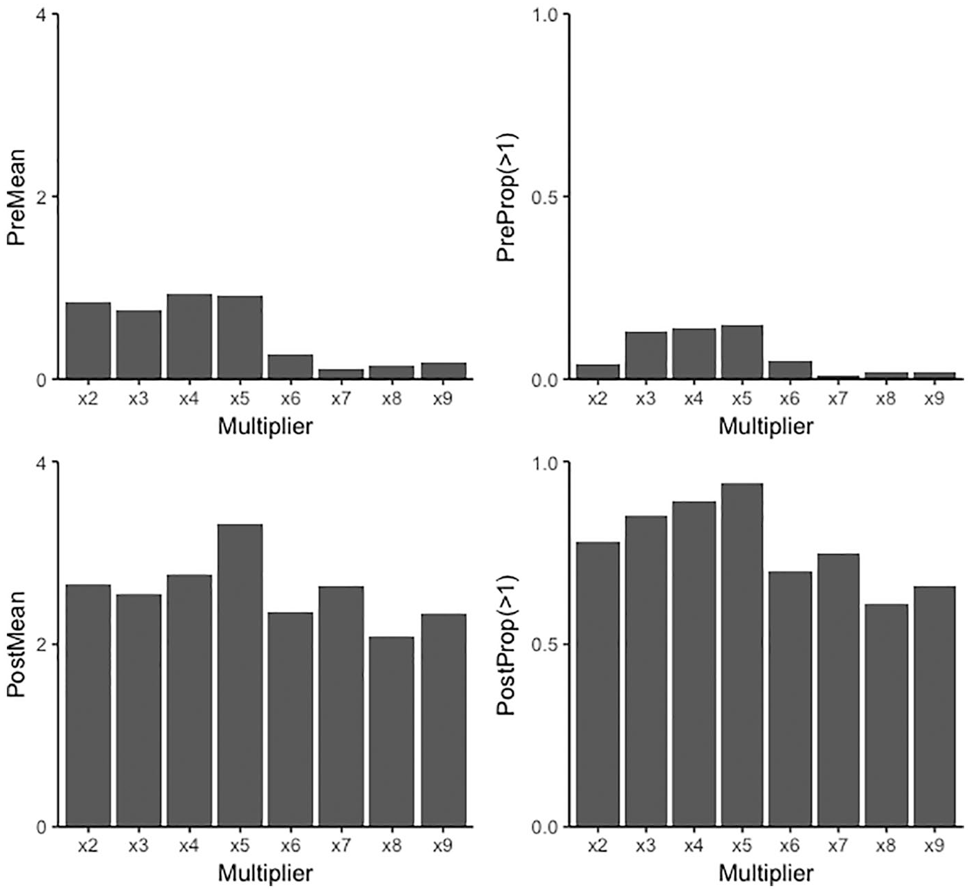
Improvement in individual multipliers from pre- to post-test. The left column shows the average amount of problems answered correctly. The right column shows the percentage of students who correctly answered at least two of the respective multiplier problems correctly, where the y-axis is pre–test proportion of students.

Study II: Influence of Set Size

Student-level analysis

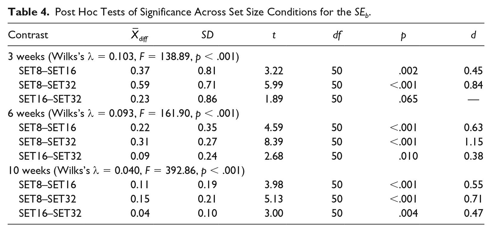
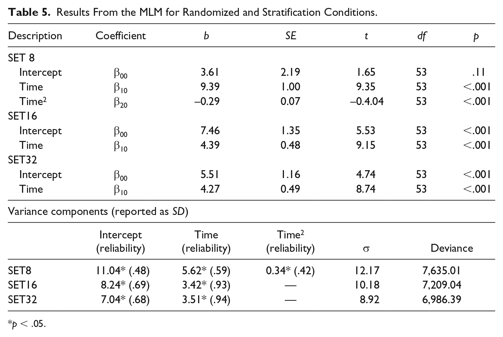
Results of the analysis of slope precision across conditions and weeks of monitoring are summarized in Table 3. Overall, the precision across sets was comparable for SET16 and SET32 probes and was observably lower for SET8 probes, which was confirmed by the ANOVA (Table 4). However, although SET8 probes yielded the highest SEE and SE_b values across all durations of monitoring, the slope of growth on these probes was also higher (Table 5), as would be expected given the narrower range of items evaluated. That is, the precision of slope relative to the average value of slope was comparable across all conditions.

Table 3.

SEE and SE_b Values Across Set Size Conditions and Progress Monitoring Durations.

	SET 8			SET 16			SET 32
Parameter	3 weeks	6 weeks	10 weeks	3 weeks	6 weeks	10 weeks	3 weeks	6 weeks	10 weeks
SEE
${\bar{X}}_{S E E} (S D)$	4.16 (1.87)	5.47 (2.16)	6.08 (1.82)	3.24 (1.78)	4.08 (1.74)	4.80 (1.69)	2.68 (1.19)	3.52 (1.19)	4.21 (1.54)
Skew_SEE	0.84	0.64	0.50	0.79	1.53	1.16	0.79	0.66	0.76
Kurt_SEE	0.49	−0.14	0.60	0.30	3.97	1.60	0.80	0.32	0.45
SE_b
${\bar{X}}_{S E_{b}} (S D)$	1.70 (0.76)	0.87 (0.35)	0.47 (0.14)	1.32 (0.73)	0.65 (0.28)	0.24 (0.12)	0.97 (0.49)	0.41 (0.21)	0.24 (0.12)
Skew_SEE	0.84	0.64	0.50	0.79	1.53	0.76	0.79	0.66	0.76
Kurt_SEE	0.49	−0.14	0.60	0.30	3.97	0.45	0.80	0.32	0.45

Note. SEE = standard error of the estimate; SE_b: standard error of beta.

Table 4.

Post Hoc Tests of Significance Across Set Size Conditions for the SE_b.

Contrast	${\bar{X}}_{d i f f}$	SD	t	df	p	d
3 weeks (Wilks’s λ = 0.103, F = 138.89, p < .001)
SET8–SET16	0.37	0.81	3.22	50	.002	0.45
SET8–SET32	0.59	0.71	5.99	50	<.001	0.84
SET16–SET32	0.23	0.86	1.89	50	.065	—
6 weeks (Wilks’s λ = 0.093, F = 161.90, p < .001)
SET8–SET16	0.22	0.35	4.59	50	<.001	0.63
SET8–SET32	0.31	0.27	8.39	50	<.001	1.15
SET16–SET32	0.09	0.24	2.68	50	.010	0.38
10 weeks (Wilks’s λ = 0.040, F = 392.86, p < .001)
SET8–SET16	0.11	0.19	3.98	50	<.001	0.55
SET8–SET32	0.15	0.21	5.13	50	<.001	0.71
SET16–SET32	0.04	0.10	3.00	50	.004	0.47

Table 5.

Results From the MLM for Randomized and Stratification Conditions.

Description	Coefficient	b	SE	t	df	p
SET 8
Intercept	β₀₀	3.61	2.19	1.65	53	.11
Time	β₁₀	9.39	1.00	9.35	53	<.001
Time²	β₂₀	−0.29	0.07	−0.4.04	53	<.001
SET16
Intercept	β₀₀	7.46	1.35	5.53	53	<.001
Time	β₁₀	4.39	0.48	9.15	53	<.001
SET32
Intercept	β₀₀	5.51	1.16	4.74	53	<.001
Time	β₁₀	4.27	0.49	8.74	53	<.001
Variance components (reported as SD)
	Intercept (reliability)	Time (reliability)	Time² (reliability)	σ	Deviance
SET8	11.04* (.48)	5.62* (.59)	0.34* (.42)	12.17	7,635.01
SET16	8.24* (.69)	3.42* (.93)	—	10.18	7,209.04
SET32	7.04* (.68)	3.51* (.94)	—	8.92	6,986.39

p < .05.

To put these values in perspective, the lowest precision for the SET8 probes for 3 weeks of monitoring was SE_b = 1.70. If one observed the average linear slope for these probes as reported in the group-level analysis, 9.39 DCPM, the 80% margin of error for this estimate after 3 weeks of monitoring (6 data points) would be ±2.19 DCPM. However, after 10 weeks, that same range would be ±0.60 DCPM. In comparison, for the SET32 data, a comparable range for 3 weeks of data would be ±1.24 DCPM, and for 10 weeks of data it would be ±0.31 DCPM.

Group-level analysis

Preliminary tests of linear and curvilinear effects suggested the SET8 condition was best explained by assuming trend was curvilinear (e.g., Time and Time²), whereas SET16 and SET32 were best modeled with only the linear predictor. Results from this analysis can be seen in Table 5, and growth on each condition, collapsed across students, is shown in Figure 2. The linear estimate suggested students grew 9.39 DCPM/week on the SET8 probes, with the associated SD of the linear effect being 5.62 DCPM. In contrast, students grew, on average, 4.39 DCPM/week on SET16 probes, and this effect also varied widely across students, SD_µ10 = 3.42. Finally, students grew, on average, 4.27 DCPM/week on the SET32 probes—this growth also being variable across students, SD_µ10 = 3.51. Slope reliability was poor for SET8 data and high for the other two conditions.

Figure 2.

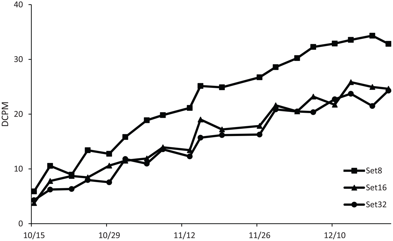
Average session-by-session growth across conditions for Study II (set size).

Discussion

The purpose of the current study was to investigate slope precision for 1 digit × 1 digit multiplication SSM-CBM probes that consisted of stratified or randomized item arrangements or that varied in the examined set size. Overall, results suggest that item arrangement and set size are meaningful considerations when designing probes for the purpose of monitoring student growth over time.

Study I

Study I evaluated whether item arrangement was influential in the precision of slope. Results of the current study demonstrated that slope estimates were more precise for the stratified condition compared with the randomized condition. Presently, a stratified item resulted in a 12% to 21% decrease in residual error relative to randomized problem assignment depending on the duration of monitoring, which is similar to the reduction in error variance found in Christ and Vining (2006) and Methe et al. (2015) for multiple-skill M-CBMs. Although inferior relative to stratified probes, randomized probes still exhibited satisfactory properties and are acceptable for research and practice. However, although there is a modest additional time cost to the preparation of stratified probes over randomized probe sets, this reduction does represent a meaningful improvement in measurement precision that is worth considering. The exact value of that benefit depends on the specified confidence interval set about the slope estimate (e.g., 80%, 90%) or, in terms of raw residual values, a gain in slope precision of about 0.50 DCPM. Such benefits translate to a better signal-to-noise ratio when monitoring outcome data over time.

As we were curious as to what pattern of difficulty across multipliers may have resulted in the observed difference in precision across conditions, we examined student data across individual multipliers. The results of our exploratory analysis confirm that there was variation in student responding, and likely difficulty, across the multipliers included on our probes. During the initial 2 weeks of data collection, students on average correctly answered more problems containing multipliers of ×2 through ×5 relative to problems containing multipliers of ×6 through ×9. In the last 2 weeks of data collection, greater variation was observed across the multipliers. For example, nearly 100% of students answered at least two ×5 multiplier questions accurately on a given probe in the final weeks, whereas only slightly more than half responded similarly to multipliers of ×8, even though instruction on ×5 and ×8 multipliers was proximally close. These varied differences in accurate responding suggest, much like multiple-skill probes, that use of randomized probes may lead to the under- or over-sampling of difficult material across administrations. Therefore, even at the single-skill level, variation in item difficulty is a pertinent consideration for assessment (Burns et al., 2015).

Finally, our group-level analysis suggests students’ response to Tier I curriculum instruction varies widely, with most growth per week falling in the range of about 1.50 to 6.50 DCPM. These differences in slope were reliable and suggest that dramatic individual changes in math fluency emerge quickly during Tier I instruction. We were expecting differences among students, but the degree of variability was both surprising and concerning. It likely behooves practitioners to periodically screen or even actively monitor all students during the time such initial instruction occurs. Fortunately, the means by which to remediate such fluency deficits are well outlined and can be executed in a short amount of time, even at the group or class-wide level (see Codding et al., 2017; Poncy et al., 2012; Schutte et al., 2015).

Study II

Our second study complemented the first by examining how represented set size affects precision of slope. As reviewed in the introduction, various empirical intervention studies have utilized different set sizes. Furthermore, researchers have encouraged applied interventionists to consider set size when planning instruction (Poncy et al., 2012). The SEE and SE_b varied across examined set sizes, with SET8 probes performing significantly worse than the other two conditions. However, when considered relative to the rates of growth observed across conditions, precision was approximately equivalent across the probe types. SET8 probes did yield other concerns, however, worth consideration. First, the multilevel model suggested that linearity should not be assumed in this situation. Nonetheless, we felt it prudent to carry this assumption in our investigation given how CBM aimlines are near universally specified in research and practice. Attesting to this misspecification of the linear model, we reran the analysis of SET8 three-week data assuming trend was modeled only as a function of the higher order polynomial, $\hat{y} = β_{0} + β_{1} {time}^{2} + e$ . The average SE_b in this case was 0.45, a 74% reduction from the linear estimate. However, interpreting curvilinear trends in practice requires greater finesse relative to a linear slope. Second, the degree of growth observed on SET8 probes suggests that the effect of testing when using small set sizes in research will be prominent and therefore, if used, should be controlled using an appropriate methodology (i.e., AB design, adapted alternating treatment design with control condition) and analysis (i.e., regression that controls for baseline trend; Moeyaert et al., 2014; Shadish et al., 2002).

The effect of time on scores for SET8 condition appeared to asymptote, on average, after about 7 weeks and just below a score a 35 DCPM, contributing to the misspecification of the linear model. Interestingly, this is just about the level of proficiency commonly perceived as representing full fluency on math single skills (30-40 DCPM; Burns et al., 2006; Codding et al., 2017; Shapiro, 2011). Perhaps a workable accommodation to address this issue in practice when monitoring individual students is to specify linear aimlines, but not to project these estimates beyond 35 DCPM. As only some students reached this level of fluency in the current study, and each at different times on different conditions, we are not able to more thoroughly address this possibility. Last, the MLM also suggested that scores from the larger set size conditions were more reliable than SET8 probes and better disentangled the relative standing of students. Overall, it appears larger set sizes are favorable, when possible and appropriate, if one wishes to project linear aimlines and engage in traditional slope-to-aimline comparisons, or if one is engaging in intervention research and using rate of growth as a primary outcome.

In Studies I and II, the duration of monitoring had a practical effect on the precision of estimation. Specifically, by extending the progress monitoring schedule from 3 to 6 weeks, the SE_b was reduced by nearly half, whereas extending the duration to 10 weeks yielded diminishing returns. Overall, the precision of slope for 6 weeks of monitoring was reasonable, ranging from an SE_b of 0.46 to 0.65, across conditions. Such precision is appreciably better than that which is commonly observed for reading CBM, where the SE_b has been observed to exceed the value of the average weekly improvement rate for small durations of monitoring (Christ, 2006). Importantly, these recommendations assume a fixed schedule of data collection twice per week.

Limitations and Future Directions

Limitations of the current study must be considered when interpreting results. First, growth and/or precision of slope may differ based on the target skill, chosen curriculum, and intensity of instruction, and future research should extend findings to additional operations and varied educational environments. Second, researchers approach probe construction in different ways. Some authors used a pseudo-randomized process, manually adjusting problems so that identical problems or identical multipliers/subtrahends/addends are not adjacent to one another after initial randomization, or they randomized within block (cf. Musti-Rao & Plati, 2015; Poncy et al., 2010, 2013). However, because of its relative popularity, we opted to use a purely randomized process in both studies, as appropriate. However, future research should examine other variations of probe construction, such as the use of block randomization or other variants of stratification. Relatedly, we investigated the main effect of stratification and set size, but the potential interaction between these two factors remains unknown and is an area for future research. Last, although we monitored the reliability of the scoring process, we did not monitor fidelity of probe administration.

Conclusion

Whereas a great deal of research has focused on reading CBM, significantly less has focused on M-CBM. Of the M-CBM research conducted, the bulk has focused on the use of multiple-skill math probes within a screening context, rather than SSM-CBMs for progress monitoring. The current study aimed to address this research gap by investigating the precision of 1 digit × 1 digit multiplication CBM, while also expanding previous research on the utility of probe stratification and the effect of the specified set size. Results demonstrated that stratified SSM-CBM probes provided more precise measures of growth for students over time relative to randomized probes, converging with prior findings. Furthermore, larger set sizes yielded more easily interpreted linearity and greater between-student reliability. Finally, 6 weeks of monitoring was observed to result in a high-level precision of slope across conditions. Therefore, we recommend that both researchers and practitioners consider item arrangements and set size relative to intervention duration when engaging in probe construction as a means to increase the signal-to-noise ratio when monitoring mastery of individual whole-number operations.

Footnotes

Acknowledgements

We wish to acknowledge additional data collectors, including Sam Sutton and Sophie Parks.

Declaration of Conflicting Interests

The author(s) declared no potential conflicts of interest with respect to the research, authorship, and/or publication of this article.

Funding

The author(s) received no financial support for the research, authorship, and/or publication of this article.

ORCID iD

Benjamin G. Solomon

References

aimsweb. (2012). Mathematics concepts and applications administration and scoring guide. Pearson Education.

Ardoin

S. P.

Christ

T. J.

(2009). Curriculum-based measurement of oral reading: Standard errors associated with progress monitoring outcomes from DIBELS, AIMSweb, and an experimental passage set. School Psychology Review, 38, 266–283.

Burns

M. K.

VanDerHeyden

A. M.

Jiban

C. L.

(2006). Assessing the instructional level for mathematics: A comparison of methods. School Psychology Review, 35, 401–418.

Burns

M. K.

Ysseldyke

Nelson

P. M.

Kanive

(2015). Number of repetitions required to retain single-digit multiplication math facts for elementary students. School Psychology Quarterly, 30, 398–405.

Christ

T. J.

(2006). Short-term estimates of growth using curriculum-based measurement of oral reading fluency: Estimating standard error of the slope to construct confidence intervals. School Psychology Review, 35, 128–133.

Christ

T. J.

Vining

(2006). Curriculum-based measurement procedures to develop multiple-skill mathematics computation probes: Evaluation of random and stratified stimulus-set arrangements. School Psychology Review, 35, 387–400.

Christ

T. J.

Zopluoglu

Monaghen

B. D.

Van Norman

E. R.

(2013). Curriculum-based measurement of oral reading: Multi-study evaluation of schedule, duration, and dataset quality on progress monitoring outcomes. Journal of School Psychology, 51, 19–57.

Codding

R. S.

Shiyko

Russo

Birch

Fanning

Jaspen

(2007). Comparing mathematics interventions: Does initial level of fluency predict intervention effectiveness? Journal of School Psychology, 45, 608–617.

Codding

R. S.

Volpe

R. J.

Poncy

B. C.

(2017). Effective math interventions: A guide to improving whole-number knowledge. The Guilford Press.

10.

Cohen

West

S. G.

Aiken

L. S.

(2003). Applied multiple regression/correlation analysis for the behavioral sciences (3rd ed.). Lawrence Erlbaum Associates.

11.

Deno

S. L.

(1985). Curriculum-based measurement: The emerging alternative. Exceptional Children, 52, 219–232.

12.

Deno

S. L.

(1986). Formative evaluation of individual student programs: A new role for school psychologists. School Psychology Review, 15, 358–374.

13.

Deno

S. L.

Mirkin

P. K.

(1977). Data-based program modification: A manual. Council for Exceptional Children.

14.

Duhon

G. J.

House

Hastings

Poncy

Solomon

(2015). Adding immediate feedback to explicit timing: An option for enhancing treatment intensity to improve mathematics fluency. Journal of Behavioral Education, 24, 74–87.

15.

Flores

M. M.

(2010). Using the concrete-representation-abstract sequence to teach subtraction with regrouping to students at risk for failure. Remedial and Special Education, 31, 195–207.

16.

Go Math! (2015). Houghton Mifflin Harcourt.

17.

Hawkins

R. O.

Musti-Rao

Hughes

Berry

McGuire

(2009). Applying a randomized interdependent group contingency component to classwide peer tutoring for multiplication fact fluency. Journal of Behavioral Education, 18, 300–318.

18.

Hintze

J. M.

Christ

T. J.

Keller

L. A.

(2002). The generalizability of CBM survey-level mathematics assessments: Just how many samples do we need? School Psychology Review, 31, 514–528.

19.

Hulac

D. M.

Dejong

Benson

(2012). Can students run their own interventions? A self-administered math fluency intervention. Psychology in the Schools, 49, 526–538.

20.

Lannie

A. L.

Martens

B. K.

(2008). Targeting performance dimensions in sequence according to the instructional hierarchy: Effects on children’s math work within a self-monitoring program. Journal of Behavioral Education, 17, 356–375.

21.

Methe

S. A.

Briesch

A. M.

Hulac

(2015). Evaluating procedures for reducing measurement error in math curriculum-based measurement probes. Assessment for Effective Intervention, 40, 99–113.

22.

Moeyaert

Ferron

J. M.

Beretvas

S. N.

Van den Noortgate

(2014). From a single-level to a multilevel analysis of single-case experimental design. Journal of School Psychology, 52, 191–211.

23.

Mong

M. D.

Mong

K. W.

(2012). The utility of brief experimental analysis and extended intervention in selecting effective mathematics interventions. Journal of Behavioral Education, 21, 99–118.

24.

Musti-Rao

Plati

(2015). Comparing two classwide interventions: Implications of using technology for increasing multipication fact fluency. Journal of Behavioral Education, 24, 418–437.

25.

National Center for Educational Statistics. (2018). The condition of education 2018. National Center for Educational Statistics, Institute of Sciences, U.S. Department of Education.

26.

Poncy

B. C.

Fontenelle

S. F.

Skinner

C. H.

(2013). Using detect, practice, and repair (DPR) to differentiate and individualize math fact instruction in a class-wide setting. Journal of Behavioral Education, 22, 211–228.

27.

Poncy

B. C.

Skinner

C. H.

Axtell

P. A.

(2010). An investigation of detect, practice, and repair to remedy math-fact deficits in a group of third-grade students. Psychology in the Schools, 47, 342–353.

28.

Poncy

B. C.

Skinner

C. H.

McCallum

(2012). A comparison of class-wide taped problems and cover, copy, and compare for enhancing mathematics fluency. Psychology in the Schools, 49, 744–755.

29.

Poncy

B. C.

Solomon

Duhon

Skinner

Moore

Simons

(2015). An analysis of learning rate and curricular scope: Caution when choosing academic interventions based on aggregated outcomes. School Psychology Review, 44, 285–305.

30.

Schutte

G. M.

Duhon

G. J.

Solomon

B. G.

Poncy

B. C.

Moore

Story

. (2015). A comparative analysis of massed vs. distributed practice on basic math fact fluency growth rates. Journal of School Psychology, 53, 149–159.

31.

Shadish

W. R.

Cook

T. D.

Campbell

D. T.

(2002). Experimental and quasi-experimental designs for generalized causal inference. Wadsworth, Cengage Learning.

32.

Shapiro

E. S.

(2011). Academic skills problems (4th ed.). The Guilford Press.

33.

Sindelar

P. T.

Rosenberg

M. S.

Wilson

R. J.

(1985). An adapted alternating treatments design for instructional research. Education and Treatment of Children, 8, 67–76.

34.

Solomon

B. G.

Dawes

J. M.

Duhon

G. J.

Poncy

B. C.

(in press). False discovery rates when engaging in skill versus performance deficit analysis for academic instructional planning. Assessment for Effective Intervention.

35.

Thornblad

S. C.

Christ

T. J.

(2014). Curriculum-based measurement of reading: Is 6 weeks of daily progress monitoring enough? School Psychology Review, 43, 19–29.

36.

Windingstad

Skinner

C. H.

Rowland

Cardin

Fearrington

J. Y.

(2009). Extending research on a math fluency building intervention: Applying taped problems in a second-grade classroom. Journal of Applied School Psychology, 25, 364–381.