Controlling Variables in Social Systems - A Structural Modelling Approach

Abstract

French

Determining the variables to be controlled for is usually a major problem in the social sciences when analyzing possible causal relations. A structural modelling approach, having recourse to directed acyclic graphs, is presented here as a consistent framework for determining a coherent set of guidelines when deciding what variables should be controlled. Two rules are developed for determining control variables when studying respectively the direct and the total effects of a cause on an outcome. An application to contraceptive use in urban Africa is given as an example. Our approach for determining control variables is simpler and more comprehensive than alternative ones based on Pearl’s back-door criterion.

Keywords

Causality Control Structural Modelling Recursive Decomposition Total Effect Direct Effect Directed Acyclic Graph

Introduction

Historically, the issue of control is typically associated with experimental practices where manipulations are performed, for instance in laboratory experiments or in randomized studies. R.A. Fisher (1935) can be considered the modern theorizer of a tradition that traces back to, at least, J.S. Mill (1843). In this context, controlling for a variable amounts to holding constant the value of that variable, e.g. repeating an experiment under different fixed levels of atmospheric pressure. In non-experimental or observational sciences, where controlled experiments are often impossible or unethical, standard textbooks in the methodology of the social sciences, such as E. Babbie (2010), R.A. Jones (2000), C. Frankfort-Nachmias and D. Nachmias (2007), or in epidemiology, such as K.J. Rothman and S. Greenland (1998), generally recommend controlling for the variables possibly having an effect on an outcome variable Y, either by intervening, when feasible, or by conditioning in a statistical model.

To see how the above recommendations are put into practice in a non-experimental science, a perusal of some recent articles in demography (see Wunsch, Mouchart, Russo, 2014) shows that, broadly speaking, in most cases the authors follow the standard recommendations. They include, based on a literature review, a vector of all known and observable possible determinants X of the outcome variable Y into a single-equation model and then consider the impact of each of these variables on the outcome Y, the other predictor variables being fixed. A distinction is often made between key explanatory variables and other variables to be controlled for. It is however not often specified whether those other variables are confounders, mediators, moderators, or independent covariates, neither is a distinction usually made between individual characteristics and contextual variables. Moreover, a theoretical framework is frequently developed in order to present the main research questions and hypotheses, though a full explanatory mechanism is most often lacking. In that sample of articles, no causal ordering of the predictor variables is generally attempted, in the sense of a structure or mechanism responsible for the outcome variable. All predictor variables are implicitly considered as if they were independent from one another (except for multi-item scales), i.e. as if different structures of association among them had no impact on the generation of the outcome variable. Some authors do however use some form of similarity analysis to examine possible groupings among variables, and interactions between variables are sometimes examined. There are of course exceptions to this approach and many other exceptions would be found if the set of texts were enlarged.

The previous selection of the literature follows to a large extent what H.-P. Blossfeld (2009) has called the causation as robust dependence approach. In this view, as discussed by D. R. Cox (1992), a variable X is a plausible cause of another variable Y if the dependence between the two cannot be eliminated by introducing additional variables in the analysis. The problem with this approach is that it is impossible to be sure that all relevant variables have been controlled for. Moreover, as H.-P. Blossfeld stresses, because covariates are often correlated, parameter estimates depend upon the specific set of variables included in the statistical model. In order to go beyond this causation via association approach, as D.R. Cox (1992) has called it, one needs what H.-P. Blossfeld (2009) has coined a causation as generative process approach. In other words, one should characterize the properties of the underlying data generating process, i.e. the mechanism behind the data. More generally, in a perspective of explanation and policy intervention, as opposed to a purely descriptive point of view, one requires understanding the plausible mechanism and sub-mechanisms generating the data in a particular context and during a specific period of time.

As the justification for inclusion of control variables is very often limited or absent in many studies (see e.g. Schjoedt and Bird, 2014), the purpose of this paper is to examine the issue of control in the perspective of a specific structural modelling of complex social systems of variables and relations, where there are multiple causes and multiple effects. In particular, this paper shows the relevant variables that have to be controlled for when studying cause-effect relations in social systems. The present paper does not deal however with methods of data collection and analysis. The order of exposition is as follows. Controlling - A Structural Modelling Perspective (section 2) briefly considers the issue of control in a structural modelling perspective, based on a recursive decomposition of a joint distribution standing for an explicit mechanism or data generating process and represented by a Directed Acyclic Graph (DAG). Controlling in the Simplest Case of 3 Variables (section 3) deals with the simplest case of three variables in a directed network and examines in this framework the variables that have to be controlled for. We then consider the issue of Controlling in More Complex Models (section 4). We derive two simple rules for selecting the variables to be controlled for in the cases of direct and total effects, without having recourse to Pearl’s back-door criterion (see e.g. Pearl, 2000). Our approach is then applied in An Example - Contraceptive Use in Urban Africa (section 5). We conclude (Discussion and Conclusions, section 6) that the real issue at stake is the modelling strategy, rather than the search for robust statistical associations.

Controlling - A Structural Modelling Perspective

In this section, the framework of structural modelling is presented as a strategy for providing an ordering of variables underlying the recursive decomposition required for attributing causes and effects and for determining the control variables. In this perspective, a structural model is a statistical model that provides a stochastic representation of a data generating process (DGP) interpreted as a global mechanism. In order to understand the functioning of this global mechanism, the latter is decomposed into an ordered sequence of sub-mechanisms congruent with background knowledge and endowed with properties of invariance or structural stability (for a discussion, see also Russo, 2014). Causal attribution is then based on such a structural model.

The structural model, as presented here, is substantially different from that developed in the literatures on structural equation models (SEM) in econometrics and in social science. In particular, the approach of this paper is not based on a system of equations, but rather on an analysis of a multivariate distribution. Moreover, the modelling stage is essentially distribution-free, the distributional hypotheses being introduced only at the estimation stage. More substantially, the usual SEM approach endeavors at representing causal knowledge while the structural perspective presented here aims at constructing causal knowledge. Thus the emphasis, in this paper, on mechanisms and sub-mechanisms, on background knowledge and on structural stability.

Our approach to structural modelling has two main origins, in econometrics on the one hand, with the work of the Cowles Commission, and in social science on the other hand, with the path analytic methodology developed by Sewall Wright. For more details, see Wunsch, Mouchart and Russo (2014). The starting point of a structural model is a set of variables X. We consider a statistical model in the form of a set of probability distributions, $M = {P_{X}^{θ} θ \in Θ}$ , where θ is a parameter characterising a probability distribution and M represents a set of plausible hypotheses concerning the data generating process (DGP). Representing the DGP by probability distributions, characterized by a parameter, implies that what is “explained” by the statistical model is embodied in the parameter whereas what is not explained is embodied in the stochastic component of the probability distributions. The structural approach blends two components. Firstly it develops a model congruent with field knowledge, in particular with explanatory theories, and stable enough with respect to a suitable class of interventions and of changes of the environment. In this sense, it provides a representation of a global mechanism, operating a distinction between structural aspects and incidental aspects of social reality. Secondly it also provides an explanation of the functioning of the social world by means of a recursive decomposition of the global mechanism in terms of an ordered sequence of sub-mechanisms.

More specifically, once the vector of variables X is decomposed into an ordered sequence of p components, namely $X = (X_{1}, X_{2}, \dots X_{p})$ (with p typically much larger than 2), a recursive decomposition is a systematic marginal-conditional decomposition of the joint distribution of X, namely:

\begin{array}{l} p_{X} (x | θ) = p_{X_{p} | X_{1}, X_{2}, \dots X_{p - 1}} (x_{p} | x_{1}, x_{2}, \dots x_{p - 1}, θ_{p | 1, \dots p - 1}) \\ \cdot p_{X_{p - 1} | X_{1}, X_{2}, \dots X_{p - 2}} (x_{p - 1} | x_{1}, x_{2}, \dots x_{p - 2}, θ_{p - 1 | 1, \dots p - 2}) \dots \\ \cdot p_{X_{j} | X_{1}, X_{2}, \dots X_{j - 1}} (x_{j} | x_{1}, x_{2}, \dots x_{j - 1}, θ_{j | 1, \dots j - 1}) \dots p_{X_{1}} (x_{1} | θ_{1}) \end{array}

where each $θ_{j | 1, \dots j - 1}$ stands for the parameters characterizing the corresponding conditional distribution $p_{X_{j} | X_{1}, X_{2}, \dots X_{j - 1}}$ . The whole recursive decomposition is interpreted as a global mechanism decomposed into an ordered sequence of acting sub-mechanisms.; more details are given in Mouchart, Russo and Wunsch (2010, 2011) and a non-technical presentation is given in Wunsch, Mouchart and Russo (2015). An example dealing with contraceptive use in urban Africa is given in section 5.

The recursive decomposition is the cornerstone of the explanatory power of a structural model because it endows the distribution $P_{X}^{θ}$ with the interpretation that each component of the decomposition, i.e. the distribution of an outcome variable conditional on its immediate explanatory variables, stands for one of the sub-mechanisms that compose the joint DGP of X. The recursive decomposition is built in such a way that the identified sub-mechanisms are interpretable from background knowledge. The order of the decomposition of X is crucial for the interpretability of the components as sub-mechanisms. In general, a recursive decomposition may be represented by a Directed Acyclic Graph (DAG) (Pearl 2000).¹

What do we mean by ‘mechanism’? In the words of Illari and Williamson (2012): “A mechanism for a phenomenon consists of entities and activities organized in such a way that they are responsible for the phenomenon”. This definition is general enough to be applicable to social contexts too. More specifically, it is compatible with an interpretation of the recursive decomposition in terms of sub-mechanisms in a structural model. In this framework, the conditioning variables are interpreted as causes within a particular sub-mechanism, in which they have a specific function or role (see Mouchart and Russo, 2011; Wunsch, Mouchart and Russo, 2014). Because a structural model, as proposed in this paper, is based on the concepts of mechanism, sub-mechanisms and functions, a characteristic feature is its ability to identify, in particular, which variables have a direct or immediate effect on each outcome considered and to deduce therefrom which variables should be controlled for, as we shall see in sections 3 and 4. In section 6, we will however discuss some shortcomings and limitations of this approach.

Controlling in the Simplest Case of 3 Variables

For expository purposes, we analyze in depth a three-variable case ( $X, Y, Z$ ) defined by a system that has been completely ordered on the basis of a structural model and represented by the DAG of Figure 1, or equivalently by a joint distribution decomposed as follows:

Figure 1.

3-variable completely ordered system

p_{X, Y, Z} (x, y, z | θ) = p_{Y | Z, X} (y | z, x, θ_{Y | Z, X}) p_{X | Z} (x | z, θ_{X | Z}) p_{Z} (z | θ_{Z})

In this equation, the parameter θ represents the characteristics of the joint distribution of $(X, Y, Z)$ and $θ_{Z}$ , $θ_{X | Z}$ , $θ_{Y | X, Z}$ stand for the characteristics of the corresponding conditional distributions.

The focus here is on the analysis of the effects of causes on outcome variables in saturated and unsaturated models. This is achieved by examining the distributions of variables considered as outcomes conditionally on their ancestors, i.e. antecedent variables in the causal sequence. An immediate cause of an outcome is called a parent of this outcome, the latter being called a child of the cause. The analysis is therefore congruent with the order of the recursive decomposition. In this structural modelling approach, the left-hand side of (2) represents an overall mechanism whereas the three terms on the right-hand side of (2) represent a decomposition of the overall mechanism into three sub-mechanisms.

The effect of a parent, for instance X or Z, on the outcome variable Y, is called a direct effect. This corresponds to the final sub-mechanism generating Y and is determined by the conditional distribution $p_{Y | Z, X}$ . Said differently, the direct effect is evaluated from the decomposition $p_{X, Y, Z} = p_{X, Z} p_{Y | Z, X}$ independently of any hypothesis on $p_{X, Z}$ . The effect of a parent, say X, on the outcome variable Y, evaluated from the conditional distribution $p_{Y | X}$ , i.e. neglecting the other parents of the outcome, in this example Z, will be called a prima facie direct effect. Later on, the effect of a non-parent ancestor will be called a total effect. It can be due to multiple directed (causal) paths from the cause to the outcome of interest or to a sole indirect path. These effects will be detailed under different hypotheses. We examine how different issues of controlling for X or for Z may arise when evaluating the effects on the outcome variable Y. We show in particular that the status of Z, or of X, as a control variable depends upon a complete specification of the model.

The Saturated Case

Figure 1 and equation (2) represent a saturated case because equation (2) represents an identity without underlying restrictions, except for the order of the variables; adding in the DAG any new directed arrow would create a cycle in the graph. In this example, Z causes X and $(Z, X)$ cause Y. Here, X is a parent of Y whereas Z is both a parent and a non-parent ancestor of Y: there is a direct path Z → Y and an indirect path Z →Y → Y from Z to Y.

The Effect of X on Y

Graphically, there is only one direct path from X to Y and Z is a confounding variable for the effect of X on Y, as it is a common cause of both X and Y. For a discussion of the concept of confounding variable or confounder, see e.g. Bollen (1989) and Wunsch (2007). Variable X is a mediator, or intermediate variable, on the indirect path from Z to Y. The variable Z appears in two conditional distributions, or sub-mechanisms, of the right-hand side of (2), namely $p_{Y | Z, X}$ and $p_{X | Z}$ .

The direct effect of the variable X on the variable Y can be described by analysing the variations of the distribution $p_{Y | X, Z}$ relatively to different values of X, but this impact depends in general upon the values of Z. For this reason, the confounding variable Z should be controlled for. This means that the variation of the distribution $p_{Y | X, Z}$ should be examined for different values of Z. As the direct effect of X on Y is characterized by the conditional distribution $p_{Y | X, Z}$ , it is important to condition the outcome on both X and Z in order to detect cases with interaction, where the direct effect of X depends upon the value of Z, as opposed to cases without interaction where the direct effect of X is not affected by the value of Z. An interaction effect is also called a moderator effect, especially in the psychological literature (Baron and Kenny, 1986). An interaction effect cannot be adequately represented in a DAG. An interaction may be due to an intrinsic non-additivity of direct effects or to neglecting, in a model, the action of other variables, as might occur when the action of these variables is unknown to the model builder or when these variables are not observable. Moreover, detecting an interaction may be a subtle issue because it may depend upon some analytical features of the model. For instance, if the conditional expectation of Y has the form $\exp {α_{0} + α_{1} X + α_{2} Z}$ , differentiating the conditional expectation reveals an interaction effect whereas the log of the conditional expectation is simply additive without interaction.

The prima facie direct effect of X on Y, captured by the conditional distribution $p_{Y | X}$ , may be viewed as an examination of the consequences of neglecting the confounding variable Z in a causal analysis. This may be due to deficiency in background knowledge or because the confounder is not observed. It may be shown that $θ_{Y | X}$ , the parameter characteristizing $p_{Y | X}$ , is actually a complex combination of the parameters characterizing the three sub-mechanisms, namely $θ_{Y | X, Z}, θ_{X | Z}$ and θ_Z. For instance, for policy purposes it would be wrong to base an intervention on the sole characteristic $θ_{Y | X}$ . Finally, the difference between the prima facie direct effect and the (controlled) direct effect may be interpreted as a supplementary effect of the confounder Z; for details, see Mouchart, Wunsch and Russo (2015). As a conclusion, controlling for Z is required for evaluating the direct effect of X but not for the prima facie direct effect of X. However, the distribution $p_{Y | X}$ may be misleading for understanding the role of X in the sub-mechanism generating Y.

The Effect of Z on Y

Graphically, there are two paths from Z to Y, a direct path and an indirect one through the variable X. In this case, the effect of Z on Y, captured by $p_{Y | Z}$ , is usually called the total effect transmitted here by the direct and indirect paths, or more generally by multiple directed (causal) paths from cause to outcome. In this example, the total effect and the prima facie direct effect of Z on Y are identical. We distinguish a total effect of Z on Y, captured by the conditional distribution $p_{Y | Z}$ , and a direct effect captured by the conditional distribution $p_{Y | X, Z}$ . Several remarks are in order. Firstly, the conditional distribution $p_{Y | Z}$ does not represent a sub-mechanism but is a mixture of two sub-mechanisms, $p_{Y | X, Z}$ and $p_{X | Z}$ . Secondly, as for the direct effect of X, the direct effect of Z on Y may be with or without interaction. Thus the variable X should be controlled for by examining the direct effect of Z for different values of X. Thirdly, the supplementary effect of Z on Y, generated by the indirect path Z → X → Y and defined as the difference between the total effect and the direct effect, depends or not upon the value of X according to whether the direct effect of Z is with or without interaction with X. Take, for instance, the very simple case where effects are measured by means of conditional expectations in a gaussian situation where² $E (Y | X, Z) = α_{0} + α_{1} X + α_{2} Z + α_{3} X Z$ and $E (Y | Z) = β_{0} + β_{1} Z$ . In this case, the supplementary effect of Z is $β_{1} - (α_{2} + α_{3} X)$ and therefore depends, or not, on X according to whether α₃ is different or equal to 0.

Unsaturated Cases

We now examine situations where Figure 1, or equation (2), has been simplified by introducing restrictions represented by deleting one of the arrows, corresponding to some form of stochastic independence.

A First Unsaturated Case - $Y ⊥ ⊥ X | Z$

In this case, Figure 1 becomes Figure 2 and equation (2) simplifies³ into:

Figure 2.

A first unsaturated case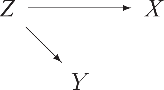

p_{X, Z, Y} = p_{Z} p_{X | Z} p_{Y | Z}

The Effect of X on Y

Without any further assumption, X and Y would not be independent. Indeed, the association between X and Y is grounded on the combined action of two sub-mechanisms represented by $p_{X | Z}$ and $p_{Y | Z}$ but disappears however once one conditions on the common cause and confounder Z, given that here $Y ⊥ ⊥ X | Z$ . The direct effect of X on Y is actually null although X and Y are not marginally independent.

The Effect of Z on Y

Under the hypothesis $Y ⊥ ⊥ X | Z$ , the direct effect of Z on Y is captured by the sub-mechanism $p_{Y | Z}$ , independently of X. The variable X should therefore not be controlled for. If, however, one did control X by examining the joint distribution of Y and Z for different values of X, namely:

p_{Y, Z | X = x_{i}} = p_{Y | Z} p_{Z | X = x_{i}}

one would find a same distribution $p_{Y | Z}$ for each value of x_i but, in the case of a discrete variable X, one would reduce the number of observations in the sub-samples corresponding to each value x_i.

A Second Unsaturated Case - $Y ⊥ ⊥ Z | X$

In this case, Figure 1 becomes Figure 3 and equation (2) simplifies into:

Figure 3.

A second unsaturated case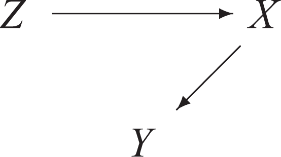

p_{X, Z, Y} = p_{Z} p_{X | Z} p_{Y | X}

The Effect of X on Y

Variable Z is not a confounder anymore and $p_{Y | X}$ is obtained directly from the decomposition of the joint distribution given by (5). In this case, the information on X is sufficient for predicting Y: adding information on Z would not improve the prediction on Y. Here, the direct effect of X on Y is correctly described by the characteristics of the conditional distribution $p_{Y | X}$ . In this situation, the direct effect of X is evaluated through $θ_{Y | X}$ , and the value of Z should not be controlled for as its effect on Y is mediated by the value of X.

The Effect of Z on Y

In this case, there is no direct effect of Z on Y because $p_{Y | X, Z} = p_{Y | X}$ and the effect of Z on Y is completely mediated by X. Moreover, for the total effect of Z, the variable X should not be controlled for because the distribution $p_{Y | Z}$ is actually a blending of two sub-mechanisms, namely $p_{Y | X}$ and $p_{X | Z}$ , where X is an active random variable.

A Third Unsaturated Case - $Z ⊥ ⊥ X$

In this case, Figure 1 becomes Figure 4 and equation (2) simplifies into:

Figure 4.

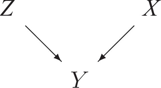
A third unsaturated case

p_{X, Z, Y} = p_{X} p_{Z} p_{Y | X, Z}

The Effect of X or Z on Y

In this case, the roles of X and of Z are perfectly symmetrical. The direct effect of X (or of Z) is evaluated through the conditional distribution of $Y | Z, X$ and the marginal independence between Z and X has no bearing on the direct effect of Z or X on Y. Changes in the distribution of Y are due, in this model, to changes in X and/or in Z. Here Z (or X) is not a confounder for the relation between X (or Z) and Y; however, variables X and Z can have an interaction effect on Y, meaning that the effect of X on Y depends upon the value of Z, and vice-versa. For this reason, it is necessary to control for, or condition on, Z (or X) when studying the impact of X (or Z) on the distribution of Y.

A General Rule for Direct Effects

Taking stock of the The Saturated Case & Unsaturated Cases sections, we have distinguished two types of paths: a direct path, e.g. Z → Y, and an indirect path, e.g. Z → X → Y. We also have distinguished several types of effects, each one being characterized by a specific conditional distribution, sometimes representing a structural sub-mechanism and sometimes not. In the saturated case, see Figure 1, one has a direct effect of a parent characterized by the final sub-mechanism and conditional distribution $p_{Y | X, Z}$ , a total effect of a non-parent ancestor, characterized by the conditional distribution $p_{Y | Z}$ , a prima facie direct effect of a parent, characterized by the conditional distribution $p_{Y | Z}$ or $p_{Y | X}$ and an indirect effect defined as the difference between a total and a direct effect of a given parent. Note that in this particular saturated case, $p_{Y | Z}$ characterized both a total effect and a prima facie direct effect of Z on Y. The selection of the variables to be controlled for depends upon the complete specification of the recursive decomposition and upon the type of effect to be considered. In particular, one should control for the possible impact of confounding and interaction.

As a general rule, if a variable has a direct effect on an outcome, one should control for, or condition on, the other variables having a direct effect on this outcome. Only these other variables should be controlled for. Basing causality analysis on the functioning of sub-mechanisms, and in particular on the parents of an outcome, we have shown that these control variables are not restricted to confounders only but also encompass the other parents leading to variations in the distribution of the outcome variable and possibly being in interaction with the causal variable.

Controlling in More Complex Models

Up to now, we have analyzed the situation of three variables, an exceedingly simple case. Once we face a more realistic situation, the issue of recursive decomposition usually becomes much more complex. Using the DAG terminology, the issue of control is raised here in the context of defining and measuring the effect of an “ancestor” variable (i.e. ancestor-parent in the case of a direct effect or ancestor-non parent in the case of a total effect), considered as a causing variable, on an outcome variable when the global mechanism is complex, i.e. involving more than 3 variables. From a structural modelling point of view, and its accompanying recursive decomposition, this issue has two facets. On the one hand, the causing variable may be a parent in the last sub-mechanism of interest generating the outcome variable conditionally on its parents (the other ancestor variables being independent of the outcome conditionally on the parents) or may be an ancestor without being a parent, upstream in the causal chain. On the other hand, when considering the sub-mechanism where a causing variable of interest is a parent, the effect of that variable also depends upon the level of the other parents in the case of interaction. Put otherwise, the issue of control is different when evaluating the effect of a non-parent ancestor on an outcome or when analyzing the effect of a parent, under the possibility of an interaction of effects of other parents. The next sections consider direct and total effects in models with more than 3 variables and propose a second general rule for determining control variables in the case of evaluating total effects.

Direct Effects in a 4-variable Case

A Saturated Model

Figure 5 presents a 4-variable saturated model where Y is an outcome of the direct effect of the other three variables. The corresponding recursive decomposition can be written as:

Figure 5.

A four-variable saturated case

p_{Z, K, X, Y} = p_{Z} p_{K | Z} p_{X | K, Z} p_{Y | K, X, Z}

Following the general rule given in A General Rule for Direct Effects, the direct effect of each of these three variables on Y requires controlling for the other two variables. Similarly, the direct effect of Z, or of K, on X, is captured by the conditional distribution

p_{X | K, Z}

and requires controlling for the other variable, respectively K or Z.

An Unsaturated Model

Consider now Figure 6, a simplification of Figure 5 obtained by the independence conditions:

Figure 6.

A four-variable unsaturated case

K ⊥ ⊥ X | Z Y ⊥ ⊥ Z | K, X

Figure 6 corresponds to the recursive decomposition:

p_{Z, K, X, Y} = p_{Z} p_{K | Z} p_{X | Z} p_{Y | K, X}

Here the sub-mechanism of interest is represented by $p_{Y | K, X}$ ; the direct effect of X (or of K) on Y may be analyzed by measuring the effect of X (or of K) on Y for different values of K (or of X) which has to be controlled for, by application of the general rule for direct effects.

Contrary to Figure 5, Z is not a parent anymore in $p_{Y | K, X}$ but is an ancestor non-parent of Y. The total effect of Z on Y, where a variation of Z will modify the conditional distributions of the parents (X and K) of Y, may be evaluated through $p_{Y | Z}$ ⁴. It should be stressed that its parameter $θ_{Y | Z}$ is, in general, a complicated function of $θ_{Y | K, X}$ , $θ_{K | Z}$ and $θ_{X | Z}$ and that $p_{Y | Z}$ does not represent in itself a structural sub-mechanism but only a tool for assessing an ancestor non-parent effect.

A 5-variable Case with Collider

Consider Figure 7, discussed in Pearl (2012). This figure corresponds to the recursive decomposition:

Figure 7.

A five-variate case

p_{V, W, Z, X, Y} = p_{V} p_{W} p_{Z | V, W} p_{X | W, Z} p_{Y | V, Z, X}

under the independence conditions:

V ⊥ ⊥ W X ⊥ ⊥ V | W, Z Y ⊥ ⊥ W | V, Z, X

Figure 7 may be viewed as an extension of Figure 1 obtained by adding the variables V and W. Notice, moreover, that, in Figure 1, controlling for Z is sufficient for evaluating the direct effect of X on Y whereas in Figure 7, it is not sufficient: V should also be controlled for, as an application of the general rule for selecting the control variables in the case of a direct effect. Evaluating the direct effect of each of the three parents of Y requires to control both of the other two parents.

Controlling only for Z may create a spurious association between V and W (indeed $V ⊥ ⊥ W$ does not imply $V ⊥ ⊥ W | Z$ ). The reader may like to compare our approach, based on the parents of an outcome, with that of Greenland, Pearl and Robins (1999) that also provides an analysis of Figure 7 on the basis of Pearl’s back-door criterion. The latter approach leads to controlling for either Z and V or Z and W in order to avoid the confounding effects of Z (common cause of X and Y) and of the association between W and V induced by the control for Z. Our approach controls for Z and V because they are parents of Y and takes accordingly care both of the confounding effects and of possible interaction effects between the direct causes of Y. Note that controlling for Z and W would take care of the confounding effects but not of the interaction effect between the two parents V and Z, at odds with the present approach. A variable such as Z, being an outcome of two parents V and W, is called a collider in the graph literature. The distributions conditional on Z do not represent sub-mechanisms and are therefore not structural, though $p_{Z | W, V}$ is.

Controlling for Latent Confounders

Latent or unobserved confounders can sometimes be controlled for by proxy variables or by instrumental ones. Pearl (2000) has devised a so-called Front-Door Criterion that can be applied for controlling a latent confounder. Consider the DAG of Figure 8. To borrow Pearl’s example, X could be smoking, Z tar deposit in the lungs, Y lung cancer, and U (unobserved) genotype. In this DAG, U is a latent confounder of the X → Z → Y path, Z being an intervening variable, or mediator, between X and Y. The parents of Y are Z and U. The DAG corresponds to the joint distribution

p_{X, Y, Z, U} = p_{U} p_{X | U} p_{Z | X} p_{Y | Z, U}

under the independence conditions

Z ⊥ ⊥ U | X

and

Y ⊥ ⊥ X | Z, U

. For measuring the (indirect) causal effect of X on Y, Pearl proposes a two-step procedure in order to control for the latent variable U (parentheses are ours). First, one computes the (direct) causal effect of X on Z, which is not confounded. Secondly, one computes the (direct) effect of Z on Y, which is however confounded by U as the latter is a common cause of Z (via X) and Y. But U can be controlled for by conditioning on X, which is on the path U → X → Z and therefore “blocks” the path from U to Z (i.e.

Z ⊥ ⊥ U | X

). These two (direct) causal effects, of X on Z and of Z on Y, can be combined in order to yield the (indirect) causal effect of X on Y controlling for U. This procedure can be applied if the set of variables Z satisfies Pearl’s front-door criterion: Z interrupts all directed paths from X to Y, there is no back-door path from X to Z, and all back-door paths from Z to Y are blocked by X. In Pearl’s terminology, a back-door path is a path between two causally ordered variables that includes an arrow pointing to the first variable, such as the path X ← U → Y from X to Y in Figure 8 (see also e.g. Morgan and Winship, 2007).

Figure 8.

Controlling for latent confounders

Actually, the non-observability of U raises two difficulties. Firstly, besides Z, U is another parent of Y. Secondly, U is also a confounder, being a common cause of Z (via X) and Y. If the confounding effect of U is indeed controlled for by Pearl’s procedure, it should be noticed however that variations in Y are due to variations in Z and to variations in U. In order to obtain the direct effect of a variation in Z on Y, net of the influence of U, one would have to cancel the effect of a variation of U on Y, i.e. also control for U as implied by the general rule for direct effects. And this is not possible, as U is latent. More importantly, and for the same reason, possible moderator effects or interactions between the causal effects of X (via Z) on Y and of U on Y cannot be examined. Pearl’s approach does not therefore completely get rid of the extraneous impact of U on the X → Z → Y relationship, even when the front-door criterion is satisfied. In such a case, there would be no complete solution unless the structural model be enlarged by adding new variables, such as e.g. parents of U that might possibly be used as proxies.

Total Effects and Control Variable Selection

Our general rule for determining the variables to control for, given in A General Rule for Direct Effects, referred to the case of the direct effect of a cause X on an outcome of interest Y. We also propose a simple rule when determining the total effect of X on Y, composed of direct and indirect effects or more generally of multiple directed, or causal, paths from cause to outcome.

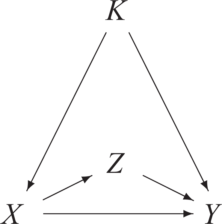
The DAG represented in figure 9 is also discussed by Pearl (2000, pp. 151-152) on the basis of his back-door criterion. In this DAG, the total effect of X on Y is transmitted by the direct path X → Y and by the indirect path X → Z → Y. As X is both a parent and a non-parent ancestor of Y, the distribution $p_{Y | X}$ characterizes a prima facie total effect of X on Y. However, this effect of X on Y is influenced by the confounder K, a common cause of both X and Y. There could also be an interaction (not considered by Pearl) between the effect of X on Y and that of K on Y. For these reasons, one should control for (or condition on) K, i.e. examine the total effect of X on Y for fixed values of K. Notice that K is not on a directed (causal) path from X to Y, though K is on a “back-door” path X ← K → Y between the two. As one sees from Figure 9, one should control for parent K of Y but not for parent Z of Y, as Z is on a directed path, in this case an indirect path, from the cause X to the outcome Y.

Figure 9.

Direct effects and control variables

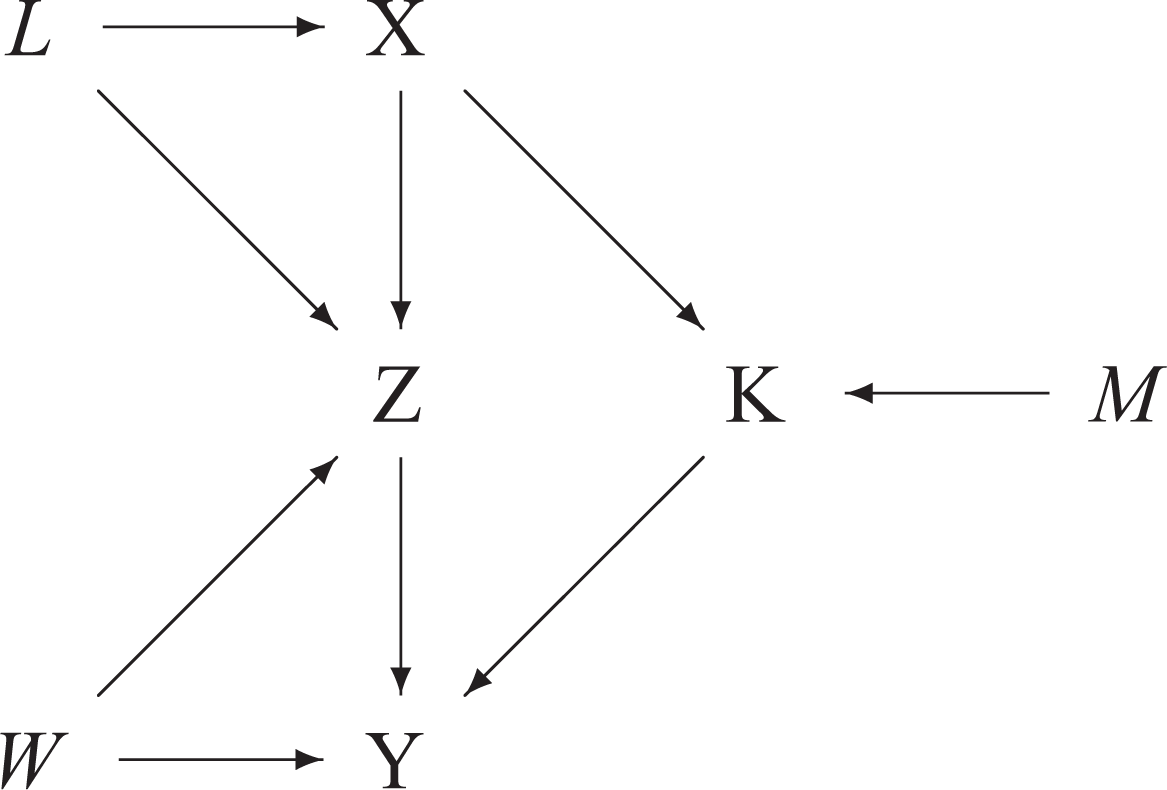
Consider now the more complex DAG of Figure 10 and suppose that one is interested in evaluating the total effect of X on Y through the mediators Z and K (the four variables are highlighted in bold). Here X is a non-parent ancestor of Y; the distribution $p_{Y | X}$ characterizes once again, a prima facie total effect of X on Y.

Figure 10.

Total effect and control variables

From the graph, one sees that the direct path X → Z is confounded by the variable L and the direct path Z → Y by the variable W. Moreover, the direct effect of M on K may be in interaction with the effect of X on K. One should therefore control for the three variables L, W, and M - parents respectively of the outcomes Z, Y, and K - by applying the general rule for determining control variables in the case of direct effects. This successive application of the rule for direct effects leads to a general rule for determining control variables when measuring the total effect of a variable X on a variable Y: One should control for all the parents of the variables on the paths from X (excluded) to Y (included), excepting these variables on the paths themselves. For example, one should control for the parents of Y excluding Z and K, which are on the indirect paths from X to Y, i.e. for variable W which is not on one of these two indirect paths. A similar reasoning applies when considering Z and K: one should respectively control for L and M, but not for X.

This suggests that the total effect of X on Y may be evaluated by comparing the conditional distributions $p_{Y | X, L = l_{i}, W = w_{j}, M = m_{k}}$ for a set of values $(l_{i}, w_{j}, m_{k})$ ⁵ This is considerably more complex than the evaluation of the total effect of X on Y based on $p_{Y | X}$ that does not take into account the interaction and confounding effects of L, W and M.

An Example - Contraceptive Use in Urban Africa

This example is based on Gourbin, Wunsch, Moreau and Guillaume (2016) and examines contraceptive use in the capital cities of four African countries, Burkina Faso, Ghana, Morocco and Senegal. The study sought to answer two questions: (i) what is the hierarchical ordering of causal relationships among the individual factors involved in contraceptive use? More particularly, (ii) given that education is a major factor in fertility transition, are the two main indirect pathways proposed in the literature (from women’s education to contraceptive use) confirmed by the data? Having recourse to a secondary analysis of Demographic and Health Survey data, the methodology is based on recursive structural models represented by directed acyclic graphs. To construct the causal model, a thorough analysis of the literature was first performed and advice taken from several experts in the field. This background knowledge showed that contraceptive use is directly dependent upon accessibility to and quality of health services, union and reproductive history, and socio-economic capital of woman and man. The latter also influences directly the two other factors and also gender relations, an intermediate factor on an indirect path between socio-economic capital and health services. The concepts incorporated into this theoretical framework were then represented by a set of relevant variables drawn from the databases. However, not all concepts had corresponding indicators in the surveys. Consequently, the concept “Accessibility to and quality of health services” was not taken into account⁶, and other concepts were only partly represented by the data at hand. Thanks to background knowledge once again, the variables were then ordered and the “parents” (i.e. direct or immediate causes) of each outcome determined, leading to the following conditional expressions (or sub-mechanisms), the symbol “|“ meaning “conditioned on”:

Woman’s contraceptive use | man’s level of education, approval of family planning, woman’s level of education, paid employment in the past twelve months, desire to have children.

Parity | woman’s age, type of union, woman’s socialization environment, length of union, woman’s level of education

Desire to have children | parity, length of union, woman’s age, paid employment in the past twelve months

Approval of family planning | age difference between spouses, man’s level of education, woman’s level of education

Woman’s age at first union | woman’s socialization environment, woman’s level of education

Length of union | woman’s age at first union

Type of union | woman’s level of education

Paid employment | woman’s level of education

Man’s level of education | woman’s level of education

Woman’s level of education | woman’s socialization environment

Age difference between spouses | woman’s level of education, man’s level of education

The exogenous variables in the global model (or mechanism) are woman’s age and her socialization environment in childhood; they are not dependent upon other variables in the model. This global model can be represented by the directed acyclic graph of Figure 11. The model was applied separately to two broad groups of birth-cohorts⁷ and to each of the four cities.

Figure 11.

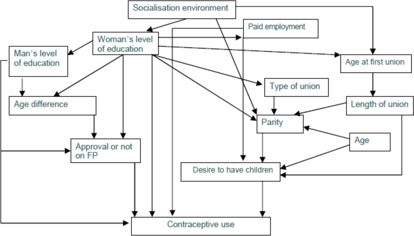
DAG of contraceptive use and its determinants

When studying the direct effect of woman’s level of education on contraceptive use, one sees - as implied by the A General Rule for Direct Effects section - that it is necessary to control (only) for man’s level of education, approval of family planning, paid employment in the past twelve months, and desire to have children. Among the indirect paths from education to contraception, two in particular are proposed in the literature: a union-reproductive path and a socio-cultural path. The first corresponds to the path: woman’s level of education → age at first union → length of union → parity → no desire to have an additional child in the next two years → contraceptive use. The second is represented by the path: woman’s level of education → man’s level of education → age difference between partners → approval of family planning → contraceptive use. Following the Total Effects and Control Variable Selection section, the indirect effect of education on contraception implies controlling (only) for the “parents” of the outcomes on the paths from education (excluded) to contraception (included), excepting these outcomes themselves. For example, for the first path and referring to the conditional expressions for the outcomes, the effect of education on age at first union (outcome 5) requires controlling for woman’s socialization environment; the effect of age at first union on length of union (outcome 6) requires no control (as there are no other parents of this outcome); and likewise for the following outcomes, including contraceptive use.

Applying piecewise logistic regressions, the study confirmed (for the four cities and both cohort groups) the union-reproductive path linking female education and contraceptive use, showing however that the effect of the former on the latter can be the reverse of what was expected. On the contrary, the analysis led to a tentative rejection of the socio-cultural path, as it was falsified by the available data. For details, limitations, and discussion, see Gourbin, Wunsch, Moreau and Guillaume (2016).

Discussion and Conclusions

The problem of control arises when defining and measuring the effect of a cause on an outcome in a complex system. The issue of control is approached, in this paper, in a specific framework of structural modelling. More explicitly, a structural model is taken here as a representation of the underlying structure of a data generating process for a well-defined population of reference. This representation is based on background knowledge, in particular in the form of some reasonably-accepted theory and well-founded observations, and checked for stability relative to a class of interventions or of changes of environment. In this framework, a complex, and therefore multivariate, global mechanism is recursively decomposed into an ordered sequence of sub-mechanisms represented by conditional distributions. A structurally valid recursive decomposition allows the modeller to interpret the conditioning variables as causes of the outcome. In this approach, the effect of a variation of a cause is to bring about a variation of the conditional distribution of the outcome, and the problem of control consists in analyzing this co-variation for different values of the variables to be controlled for.

For an outcome of a sub-mechanism of interest, the recursive nature of the decomposition leads to distinguishing between parents and ancestors of the outcome and to recognize the possibility of multiple paths from an ancestor variable to the outcome of interest. Focusing specifically on the outcome variables, two general rules are proposed for deciding what variables to control for. Concerning firstly the direct effect of a parent X on an outcome of interest Y, control variables are those other parents of Y that have a direct effect on the outcome. Secondly, concerning the total effect (e.g. in the case of multiple causal paths) of an ancestor variable X on an outcome of interest Y , control variables are those parents of the variables on the paths from X (excluded) to Y (included), excepting these variables on the paths themselves. The set of variables to be controlled for is thus larger than that of confounders determined by Pearl’s back-door criterion. These rules take however exception with the statement, recalled in the Introduction, that one should control for all variables possibly having an effect on the outcome of interest, as the present approach restricts the set of variables to be controlled for to a subset of the ancestors of the outcome.

Controlling thus means examining the behaviour of conditional distributions that represent sub-mechanisms under different values of the control variable(s). These values may however result from two different procedures. A first procedure conditions on different values of the control variable and may accordingly be called controlling by conditioning. This operation is made on a given (structural) model and does not affect the structure of the model, as it is independent of its empirical basis. This approach, based on standard rules of probability theory, is often used with observational data but could also be used with experimental data. Another procedure intervenes in the global mechanism by fixing the values of the variable to be controlled for. It can be called controlling by intervention. For some authors, such as D.B. Rubin and P.W. Holland (Holland, 1986), there is no causation without manipulation, i.e. intervention. It should be noted that controlling by intervention implies a modification of the DGP: the variable to be controlled for is not generated anymore by the sub-mechanism identified in the recursive decomposition, but by the intervention itself. As pointed out by Lucas (1976), and often overlooked in the literature on causality, such a modification of the sub-mechanism may also lead to modifying other sub-mechanisms, in particular when the intervention is operated under a change of policy active on the global mechanism. This is not the case in the controlling by conditioning approach, where no changes are brought to the DGP.

Various important caveats have however to be pointed out. Some DGPs, such as Newton’s law of gravitation, are possibly not recursive. Other DGPs could possibly be recursive but background information is insufficient for building the structural model and the corresponding DAG. For example, several explanations of the fertility transition have been offered in the literature but there is no consensus among demographers on the correct mechanism. In this situation, checking whether one hypothesis leads to more stable mechanisms than another hypothesis may be particularly relevant but does not always provide a conclusive answer to this challenge. In other cases, a structural model can be proposed but the data are unavailable for some of the variables in the model and these remain latent. This is also the case with time-dependent feedback models, which are recursive but where data are lacking on the accurate timing of causes and outcomes.

Sub-mechanisms have to be clearly spelled out and justified, and the role-function of each variable in the sub-mechanism must be given. If there are several paths from cause to outcome, such as in An Example - Contraceptive Use in Urban Africa, one should state whether exposed individuals can follow several paths together or whether these paths are mutually exclusive. Structural models, and the causal inferences derived from them, refer to a population and not to an individual. At the individual level, one cannot experience at the same time both the putative cause and its counterfactual, e.g. taking aspirin to recover from a cold and not taking aspirin. At the population level this is however not true: for colds, some individuals take aspirin and others do not, and an important issue here is to take into account the fact that the individuals in the two groups possibly differ on other factors too, populations being heterogeneous. Thus, in this paper the focus has been on conditional probability distributions instead of solely on their characteristics, such as the conditional expectation (e.g. the expected number of children per woman).

To conclude, there are no conditional independencies that alone tell us whether a variable is a control variable that has to be included in the model. Such decisions are taken, to the best of our knowledge, on the basis of background information, of preliminary analyses of data and of the structural model that is accordingly proposed. “To the best of our knowledge” implies keeping open the possibility of improving the structural model by incorporating innovations in the field of data, theory and methods. In particular, the progress of knowledge can lead to uncovering previously unrecognised control variables and unrecognised mechanisms.

Footnotes

Acknowledgements

The authors thank Thomas Baudin, Catherine Gourbin, Malgorzata Mikucka, and Joniada Milla, for valuable comments and suggestions on an earlier version of this paper. Moreover, comments by anonymous referees of this journal have helped the authors to improve the quality of their exposition.

Declaration of Conflicting Interests

The author(s) declared no potential conflicts of interest with respect to the research, authorship, and/or publication of this article.

Funding

The author(s) received no financial support for the research, authorship, and/or publication of this article.

Notes

References

Babbie

E. R.

(2010) The practice of social research, Wadsworth, Belmont.

Baron

R. M.

Kenny

D. A.

(1986) The moderator-mediator variable distinction in social psychological research: Conceptual, strategic, and statistical considerations, Journal of Personality and Social Psychology, 51, 1173–1182.

Blossfeld

H.-P.

(2009) Causation as a generative process, Chapter 5 in: Engelhardt

Kohler

H.-P.

Fürnkranz-Prskawetz

. (eds.), Causal analysis in population studies, Springer, 83–109.

Bollen

K.A.

(1989) Structural Equations with Latent Variables, John Wiley & Sons, New York.

Cox

D.R.

(1992) Causality: some statistical aspects, Journal of the Royal Statistical Society, Series A, 155(2), 291–301.

Fisher

R. A.

(1935, 1st edition) The design of experiments, Edinburgh: Oliver & Boyd.

Frankfort-Nachmias

Nachmias

(2007) Research methods in the social sciences, Worth Publishers, Gordonsville.

Gourbin

Wunsch

Moreau

Guillaume

(2016) Direct and indirect paths leading to contraceptive use in urban Africa. An application to Burkina Faso, Ghana, Morocco, Senegal, Revue Quetelet, under revision.

Greenland

Pearl

Robins

J.M.

(1999) Causal diagrams for epidemiological research, Epidemiology, 10(1), 37–48.

10.

Holland

P.W.

(1986) Statistics and Causal Inference, Journal of the American Statistical Association, 81(396), 945–960.

11.

Illari

P. M.

Williamson

(2012) What is a mechanism? Thinking about mechanisms across the sciences, European Journal for Philosophy of Science, 2 (1), 119–135.

12.

Jones

R. A.

(2000) Méthodes de recherche en sciences humaines, De Boeck, Brussels.

13.

Lucas

(1976) Econometric Policy Evaluation: A Critique. In: Bruner

Metzler

The Phillips Curve and Labour Markets, Carnegie-Rochester Conference Series on Public Policy, 1, New York: American Elsevier, 19–46.

14.

Mill

J. S.

(1843) A System of Logic, Ratiocinative and Inductive: Being a Connected View of the Principles of Evidence and the Methods of Scientific Investigation, (Seventh (1868) edn), Longmans, Green, Reader, and Dyer, London.

15.

Morgan

S.L.

Winship

(2007) Counterfactuals and Causal Inference, Cambridge University Press, New York.

16.

Mouchart

Russo

Wunsch

(2010) Inferring Causal Relations by Modelling Structures, Statistica, LXX(4), 411–432.

17.

Mouchart

Russo

(2011) Causal explanation: recursive decompositions and mechanisms, in McKay Illari

Russo

Williamson

(eds), Causality in the sciences, Oxford University Press, Oxford, 317–337.

18.

Mouchart

Russo

Wunsch

(2011) Structural modelling, Exogeneity and Causality Chapter 4 in: Engelhardt

Kohler

H.-P.

Fürnkranz-Prskawetz

, Causal analysis in population studies, Springer, 59–82.

19.

Mouchart

Wunsch

Russo

(2015) The issue of control in multivariate systems, A contribution of structural modelling, Discussion Paper DP2015/19, Institute of Statistics, Biostatistics and Actuarial Sciences (ISBA), Université catholique de Louvain, http://dial.uclouvain.be/handle/boreal:162165?site_name=UCL

20.

Pearl

(2000) Causality. Models, Reasoning, and Inference, Cambridge University Press, Cambridge, revised and enlarged in 2009.

21.

Pearl

(2012) The Mediation Formula: A guide to the assessment of causal pathways in nonlinear models, in Berzuini

Dawid

A. P.

Bernardinelli

(eds.) Causality: Statistical Perspectives and Applications, Wiley, Chichester, 151–179.

22.

Rothman

K.J.

Greenland

(1998) Modern Epidemiology, 2nd edition, Lippincott-Raven, Philadelphia.

23.

Russo

.(2014) What invariance is and how to test for it, International Studies in Philosophy of Science, 28(2), 157–183, DOI: 10.1080/02698595.2014.932528

24.

Schjoedt

Bird

(2014) Control variables: use, misuse and recommended use, in Carsrud

Brännback

(eds.) Handbook of Research Methods and Applications in Entrepreneurship and Small Business, Edward Elgar, Cheltenham, 136–155.

25.

Wunsch

(2007) Confounding and Control, Demographic Research, 16, pp. 15–35.

26.

Wunsch

Mouchart

Russo

(2014) Functions and mechanisms in structural-modelling explanations, Journal for General Philosophy of Science, 45, 187–208.

27.

Wunsch

Mouchart

Russo

(2015) Les limites de la connaissance en sciences sociales. L’explication mise en cause, Collection L’Académie en poche, Académie Royale de Belgique, Bruxelles.

Controlling Variables in Social Systems - A Structural Modelling Approach

Abstract

Keywords

Introduction

Controlling - A Structural Modelling Perspective

Controlling in the Simplest Case of 3 Variables

The Saturated Case

The Effect of X on Y

The Effect of Z on Y

Unsaturated Cases

A First Unsaturated Case - Y ⊥ ⊥ X | Z

The Effect of X on Y

The Effect of Z on Y

A Second Unsaturated Case - Y ⊥ ⊥ Z | X

The Effect of X on Y

The Effect of Z on Y

A Third Unsaturated Case - Z ⊥ ⊥ X

The Effect of X or Z on Y

A General Rule for Direct Effects

Controlling in More Complex Models

Direct Effects in a 4-variable Case

A Saturated Model

An Unsaturated Model

A 5-variable Case with Collider

Controlling for Latent Confounders

Total Effects and Control Variable Selection

An Example - Contraceptive Use in Urban Africa

Discussion and Conclusions

Footnotes

Acknowledgements

Declaration of Conflicting Interests

Funding

Notes

References

A First Unsaturated Case - $Y ⊥ ⊥ X | Z$

A Second Unsaturated Case - $Y ⊥ ⊥ Z | X$

A Third Unsaturated Case - $Z ⊥ ⊥ X$